MOCCA: Measure of Confidence for Corpus Analysis - Automatic Reliability
Check of Transcript and Automatic Segmentation
Thomas Kisler, Florian Schiel
Institute of Phonetics and Speech ProcessingSchellingstr. 3, 80799 M¨unchen, Germany {kisler, schiel}@bas.uni-muenchen.de
Abstract
The production of speech corpora typically involves manual labor to verify and correct the output of automatic transcription/segmentation processes. This study investigates the possibility of speeding up this correction process using techniques borrowed from automatic speech recognition to predict the location of transcription or segmentation errors in the signal. This was achieved with functionals of features derived from a typical Hidden Markov Model (HMM)-based speech segmentation system and a classification/regression approach based on Support Vector Machine (SVM)/Support Vector Regression (SVR) and Random Forest (RF). Classifiers were tuned in a 10-fold cross validation on an annotated corpus of spontaneous speech. Tests on an independent speech corpus from a different domain showed that transcription errors were predicted with an accuracy of 78% using an SVM, while segmentation errors were predicted in the form of an overlap-measure which showed a Pearson correlation of0.64to a ground truth using SVR. The methods described here will be implemented as free-to-use Common Language and Resources and Technology Infrastucture (CLARIN) web services.
Keywords:automatic segmentation, MAUS, confidence measure
1.
Introduction
The creation of a new speech corpus typically involves three major steps: (1) recording, (2) (orthographic) tran-scription and (3) alignment of the trantran-scription to the recorded signal, referred to hereafter as segmentation and labeling (S&L). The quality of these three production steps more or less defines the usefulness of the speech resource. The transcription of a speech recording (2) can be done ei-ther manually or via Automatic Speech Recognition (ASR). In both cases the transcription may contain errors in the form of deviations between the transcribed words and the words that were actually spoken. The S&L (3) can also be done either manually or automatically based on the tran-script created at step (2). Since manual S&L is more time-consuming than (2) (slower by a factor of around 20 to 100), step (3) is often first done automatically (applying text-to-speech alignment or similar techniques) and then manually corrected afterwards. Both tasks – the manual correction of the transcript or the manual correction of the S&L – are expensive and time-consuming because every part of every utterance must be checked manually.
This study is concerned with the automatic and reliable de-tection of errors in the S&L either caused by falsely tran-scribed words1 or by errors of the applied S&L system:
Measure of Confidence for Corpus Analysis (MOCCA). More specifically, MOCCA consists of two methods for the reliable detection of word errors in the transcription and for the word-by-word estimation of the quality of the S&L in the form of an overlap measure. Both MOCCA meth-ods can be used to automatically identify parts in the S&L where ’something went wrong’, and thus facilitate the man-ual correction task.
The estimation of the correctness of a word label in a tran-scription based on the speech signal is similar to the
as-1Note that for the purpose of this study it is irrelevant whether
these errors stem from ASR or a manual transcription
sessment of a hypothesized word in ASR systems during or after recognition. In ASR research such confidence mea-sures have attracted significant attention and have been used to detect recognition errors or to detect out-of-vocabulary (OOV) words. Good overviews for confidence measures are Jiang (2005) and Seigel (2013). Both classify confi-dence measures into three categories: 1) theposterior prob-ability approach, which estimates the true posterior proba-bilities by approximating the probability mass function of all possible acoustic feature vectors, 2) theutterance veri-fication approach, which treats the problem of confidence estimation as a statistical hypothesis testing problem (using Likelihood Ratio Testing), where an approximation of the alternate hypothesis is needed for a reliable decision, and 3) theclassification approach, in which a model is trained to estimate whether or not a word is correctly recognized. Kemp et al. (1997) applied aclassification approachwith a linear classifier and a neural net on features that were ex-tracted from the ASR decoder process. As Zhang and Rud-nicky (2001) and also Seigel (2013) pointed out, a funda-mental problem of ASR decoder features is that the features to generate the hypotheses and the features that are used to make the prediction about the quality of those hypotheses are the same, and are therefore not optimal to assess the quality of the ASR output in a post-processing step. This fundamental problem does not apply in our case because the S&L system has two inputs: the speech signal and the transcript, which is produced independently from the S&L decoding.
Paulo and Oliveira (2004) used features from a forced-alignment system to estimate the quality of automatic S&L. They estimated a measure called the Overlap Ratio (OvR), in which the overlap on phoneme level was estimated (cf. section 4.2.). In contrast to that earlier study, we aim to estimate the OvR over a complete word.
features (Kemp et al., 1997), for example the number of times the model switches to a lower N-gram model, or the number of active final word states. Therefore we use a sub-set of the features described in Kemp et al. (1997) that were suitable for the present study and could be extracted without additional processing (e.g. estimating the Signal-to-Noise ratio of a word segment, etc.).
The remainder of this paper is organized as follows: the next section briefly describes the basic experimental setup, the S&L system to be evaluated, the features used and the classifiers that were applied. Section 3. outlines the speech data on which we test the proposed MOCCA methods, and in section 4. we describe the two experiments and discuss their results.
2.
Method
2.1.
Overview
The MOCCA tagger was based on a classification ap-proach, which introduces a post-processing step after the actual alignment. The general setup of the experiments was as follows: test data consisting of the speech signal and the corresponding transcript were processed by the S&L sys-tem Munich AUtomatic Segmentation Syssys-tem (MAUS) de-scribed in Schiel (1999). Based on features derived from the MAUS decoding process, MOCCA tagged each word of the input transcript as to whether it matched the speech signal or not (experiment 1) and at the same time estimated the degree of overlap (OvR) between the calculated seg-mentation and the ground truth segseg-mentation (experiment 2). The estimation of whether a word label is correct is a two-class classification problem, while the prediction of the OvR is a regression task; for both tasks, classification and prediction, we tested a SVM, which was reported to give good results in Zhang and Rudnicky (2001), and a RF.
2.2.
S&L System MAUS
The transcript text input was converted into a canonical phonological transcript using the grapheme-to-phoneme service G2P (Reichel, 2012). The phonological transcript was then passed to the MAUS service, which first gener-ated a probability graph for all predictable pronunciations together with their prior probabilities (Schiel, 2015), and then decoded this graph into the most likely S&L using the Hidden Markov Toolkit (HTK, Young et al. (2002); for details about the MAUS technique see Schiel (1999)). Features for the confidence measure experiments were ex-tracted from the HTK Viterbi decoding as described in the following section.
2.3.
Features
Kemp et al. (1997) showed that features from the output of an ASR system can be utilized to predict the correctness of the recognized words. Since the automatic segmentation obtained with MAUS is not exactly the same as the output of an ASR system, only a subset of the features described in Kemp et al. (1997) were extracted for each segmented word:
logLM: the log prior language model probability
logAP: the log posterior probability as produced by the HTK Viterbi decoder (Young et al., 2002)
logAPNorm: the log posterior probability normalized by log prior probability:
logAP N orm=logAP −logLM
Duration: the duration after alignment of the phoneme se-quence as output by G2P of the segmented word SpkRate: the local speaking rate, calculated as the ratio
of the mean phoneme sequence duration of the word in the training dataM eanDurationandDuration:
SpkRate=M eanDurationDuration
logNPhones: the logarithm of the number of phonemes in the target word according to segmentation
The MAUS system models phones not words. Since words have variable numbers of phonesn, it follows that for each word,nfeature valueslogLM,logAPandlogAPNormare produced. To circumvent the problem of feature vectors with variable lengths, we used the following functionals of these features: sum, mean, median, range, standard devia-tion, varianceandDiscrete Cosine Transform (DCT) coef-ficients 1-3.
• sum:sum(X) =
n
P
i=1
xi
• mean:X = 1
n n
P
i=1
xi
• median:med(X) =
(
xn+1
2 nodd
1
2 xn2 +xn+12
neven
• range:range(X) = max(x)−min(x)
• standard deviation:σ(X) =
s n
P
i=1
(xi−x)2
N−1
• variance:V ar(X) =σ2
• DCT coefficients 1-3: Ck(X) = n
P
i=1
xicos [πn(i+12)k], fork= 1,2,3
wherenis the number of phonemes andxi is the feature
value of thei−thphoneme of a given feature. This yields a feature vector of constant dimensionalityp= 30for each word.
2.4.
Classifiers
For both experiments we tested two different classifica-tion/regression algorithms: SVM and RF (Meyer et al., 2015; Wright and Ziegler, 2015). Both classifiers sup-port binary classification and regression (with minor dif-ferences, e.g. the splitting criterion).
SVM The two best SVM kernels reported in Zhang and Rudnicky (2001) were a Gaussian Radial Basis Function (RBF) kernel of the form:
k(u, v) =exp(−γku−vk2) (1)
and the ANOVA RBF kernel of the form:
k(u, v) =
n
X
k=1
Since the training of the ANOVA kernel is quite time-consuming, and Karatzoglou et al. (2005) report that ANOVA RBF kernels generally perform well in regression problems, we applied this kernel only for the regression task in experiment 2. The Gaussian RBF kernel was ap-plied in both experiments 1 and 2.
Since the SVM is sensitive to its hyperparameters, we tuned them by performing a standard grid search: in the case of the Gaussian RBF kernel, we tuned the parametersC (val-ues tested: C = 0.0001,0.001,0.01,0.1,1,10,100) and
γ(values tested: γ = 0.0001,0.001,0.01,0.1,1,10,100). For the ANOVA RBF kernel we tuned the parameters C
(values tested: C = 0.1,1,10), σ (values tested: σ = 0.1,1,10) anddegree(values tested:degree= 1,2,3). For implementation we applied the R Programming Lan-guage (R) packagee1071(Meyer et al., 2015) which uses theLibSVMlibrary (Chang and Lin, 2011), a parallelizable implementation of SVMs.
Random Forest Fern´andez-Delgado et al. (2014) showed that RFs often have similar or better performance in classification problems than SVMs. Additionally, RFs have the advantage that they are less sensitive to their (tunable) parameters (Breiman, 2001; Archer and Kimes, 2008; D´ıaz-Uriarte and De Andres, 2006), and that they can be parallelized more efficiently than SVM. The two RF parameters we tuned were the number of trees to grow (ntree = 50,100,200,500) and the number of features to consider at each split in the tree (mtry=√p,8,p3). We used theRpackageRandom Forest Generator (ranger) to train the random forests, since ranger is to our knowledge the fastest RF implementation available in R (Wright and Ziegler, 2015).
3.
Test Data
We tested MOCCA on recordings from two different speech corpora. For training and parameter tuning in a 10-fold Cross Validation (CV)2 we used a subset of the Kiel
Corpus (Kohler, 1995). To evaluate the performance of MOCCA, we used recordings from the PhonDat2 (PD2) corpus (The ASR Consortium, 1995) as an independent test set. Both corpora have a manually verified ortho-graphic transcript and a manual S&L which was produced by trained phoneticians. Both corpora contain German read and spontaneous speech produced by native German speak-ers.
Kiel Corpus: The subset of the Kiel corpus used in the present study consists of 2225 utterances from spontaneous speech produced by 30 speakers doing the appointment scheduling task and while performing a map task3 (John,
2012).
PD2 The subset of the PD2 corpus used in the present study consists of read speech produced by 16 speakers, who each produced 64 semi-spontaneous utterances doing an information query task (1024 utterances total).
2
In each fold a speaker is either part of the test or training set and the number of observations is balanced so that each of the 10 test and 10 training sets has roughly the same size.
3For a detailed description of a map task please refer to
(An-derson et al., 1991)
4.
Experiments and Results
4.1.
Experiment 1: Correctness of Transcription
Overview: This section describes experiment 1, the goal of which was to correctly recognize, whether a word in the given transcript is correct or not. An example of the assign-ment of correct confidence measure labels to an incorrect transcript can be found in Table 1.
In this section we tested the following hypothesis: The fea-tures described in section 2.3. carry enough information to classify each segmented word into the classes ’correct tran-script’ versus ’incorrect trantran-script’. Since there were no transcription errors in the test sets, we applied a replace-ment strategy on every test recording to introduce artifi-cial transcription errors as explained in the following para-graphs.
Real utterance: Have a great day Confidence Measure Label: C C I C
Given Transcription: Have a bad day
Table 1: Illustration of the mode of operation of MOCCA by labeling incorrectly transcribed parts of speech (correct: C; incorrect:I).
Artificial Transcription Errors: First a MAUS S&L was performed on the test recording and features were ex-tracted from the decoder output for all words. Since we assume that the transcript is correct, these features repre-sent the “correct transcript” case. We then repeated the S&L over the complete recording, once for each wordwo
that had an OvR (see section 4.2.) of more than 90% be-tween the MAUS S&L and the ground truth segmentation, but withwo replaced by another (wrong) word wr in the
transcript. Again, features were extracted from the decoder output for the replaced wordwr, this time representing the
“incorrect transcript” case.wrwas randomly selected from
the corpus’ word list with two restrictions: first, the number of characterslength(wr)had to be in the range of±1
com-pared to the length of original wordlength(wo); second,
the word-length normalized Levenshtein distance (Leven-shtein, 1966) betweenwrandwohad to be at least 75%. If
no word could be found in the range±1, the range was in-crementally increased, until a replacement could be made. For example, a rejected replacement for “train” would be “rain”, since “rain” only fulfills the length requirement and not the Levenshtein requirement; a valid replacement for “train” would be for instance “wash”.
The word length restriction was introduced so that replace-ment words had roughly the same amount of phonemes. This is crucial in cases for words that are originally very short and are replaced by much longer words e.g. “ja” by “Zugverbindung” (“yes” by “train connection”). In this case the MAUS S&L may fail, since the available time frame is too short for the number of phonemes to be aligned.
and the replacement word. Although this probably simpli-fied the recognition task to a certain degree, it allows us to test the feasibility of transcription error detection based on features from the Viterbi decoder in the first place.4
This replacement strategy had two benefits: firstly, many training examples could be generated automatically, and secondly the training set was balanced with regard to the output classes (every word in the transcript was analyzed once as correct and once as incorrect). The procedure ap-plied to the test data yielded a total of 26,649 training ex-amples.
Results: Table 2 summarizes the results of the classifica-tion. Hyperparameters of both classifiers were optimized to a 10-fold CV of Kiel Corpus (see values in the caption of Table 2). We report accuracy, precision and recall for the model yielding the best accuracy, defined as:
Accuracy= tp+tn
tp+tn+fp+fn
Precision= tp
tp+fp
, Recall= tp
tp+fn
where tp are the true positives, tn the true negatives, fp
the false positives andfnthe false negatives (“bad” is the
positive class).
The lower half of 2 shows the results for tests on the inde-pendent test set PD2 using the same parametrization.
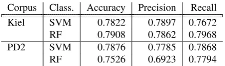
Corpus Class. Accuracy Precision Recall
Kiel SVM 0.7822 0.7897 0.7672
RF 0.7908 0.7862 0.7968
PD2 SVM 0.7876 0.7785 0.7868
[image:4.595.89.250.274.327.2]RF 0.7526 0.6923 0.7794
Table 2: Results of the classifiers SVM and RF, when tuned to the Kiel corpus (maximal accuracy); the SVM was built with tuned parametersC = 100andγ = 0.1; the RF was built with parametersntree= 500andmtry= 8.
The SVM and the RF both showed similar performance metrics in the 10-fold CV (Kiel); the RF had a slightly bet-ter accuracy than the SVM. This result is consistent with Fern´andez-Delgado et al. (2014) who also found that RFs and SVMs had similar accuracies in classification tasks. When testing against the independent test set PD2, the ac-curacy obtained for the SVM was very close to the one on the Kiel data set; it therefore seems that the SVM gener-alized better than the RF. The RF also showed a skewed distribution towards predicting more false negative results
fnwhich lead to a decrease in precision by more than 10%
on the independent data set.
Example: An example can be seen in Table 3, where MOCCA used the best SVM model to predict the correct-ness of each word in a transcript taken from the PD2 cor-pus. The classification results of two transcripts are shown: one correct (top) and one where the word “es” (“it”) was
4
It would be interesting to measure the Levenshtein distance in real data, and study how this influences the outcome of the error detection, but at the time of writing such data were not available.
replaced by “man” (“one”) following the replacement strat-egy described in section (bottom). In both cases the aligned transcript is shown together with class probabilities and classification result of the SVM.
As expected the class probability was decreased for the re-placed word in the wrong transcript (underlined). Addi-tionally, the class probability for the following word was decreased as well. This is due to the fact that the wrong transcript also influenced the segmentation of the following word.
Class prob.: 0.9299 0.7325 0.7523 0.7225
Class labels: C C C C
Correct Transcr.: Geht es nicht eher Wrong Transcr.: Geht man nicht eher
Class labels: C I C C
[image:4.595.51.271.397.462.2]Class prob.: 0.9330 0.1252 0.6821 0.7225
Table 3: A real live example from the PD2 corpus of the German sentence “Geht es nicht eher” (which loosely trans-lates in this context to “Isn’t there an earlier connection”). The replaced (wrong) word in the transcript is underlined (see text for details).
4.2.
Experiment 2: Segmentation Quality
Figure 1: A real example of phoneme strings and their alignment: an automatic and erroneous S&L (top), a man-ual and correct S&L (bottom) and the resulting OvR values (middle).
Overview: In this experiment the predictive power of the extracted features (cf. Section 2.3.) with regard to the segmentation quality was evaluated by predicting the val-ues for the OvR and comparing these to the OvR from the ground truth segmentation.
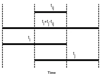
The OvR is a measure of the amount of overlap between two given time segments. It is independent of the dura-tion of the segmentstiandtj and is defined as (Paulo and
Oliveira, 2004):
OvR= tij
ti+tj−tij
(3)
whereti andtj are the duration of the segments iand j
respectively (see Figure 2).
The range of the OvR is from]− ∞,1]. However, in our case it made no difference whether something was “nega-tively overlapped” (OvR < 0), meaning that a gap existed between the segments, orOvR = 0, meaning that the end of segmenttiwas the beginning of segmenttj. We
[image:4.595.306.540.399.460.2]Figure 2: The visualization of the OvR as described in equation 3 (adapted from Paulo and Oliveira (2004)).
OvR became[0,1](where 1: perfect match of segment to ground truth; 0: total mismatch).
Unfortunately the overlap ratio was not equally distributed over the possible range of values: there were very many val-ues close to 1 (indicating an almost total overlap of word segments to the ground truth segmentation) and very few values<1(indicating a small overlap). While this is actu-ally a good sign since it means that the MAUS S&L was in most cases correct, it made it difficult to train a model that can predict the OvR equally well over the complete range of possible values.
Binning: To address this problem we divided the OvR into 20 equally sized bins of width 0.05between0and1
and restricted all bins to the same number of measurements. We set this number of measurements to the average over all bins (1890observations), and selected these randomly from the available measurements. This corresponds to an under-sampling strategy, in which the bins with a higher number of observations are under-sampled more often than the bins with fewer observations. This strategy resulted in a total of 55,739 training observations from the Kiel Corpus.
Results: Table 4 summarizes the results for the SVR as well as the RF. The values reported are the Pearson cor-relation coefficient between real and predicted OvR (Cor-Coeff), mean absolute error (MAE), and root mean squared error (RMSE). Again we only report values resulting from the best parametrization of the hyperparameters (see cap-tion), in this case tuned according to the correlation coef-ficient (CorCoeff). The results of the ANOVA RBF kernel were omitted, because the best parametrization of the SVR model based on a standard hyperparameter grid search re-sulted in a weak negative correlation (−0.26).
The results were again very similar for the SVR and RF regression in the cross validation (Kiel). When applied to the independent test set (PD2), the correlation significantly decreased for all classifiers, which indicates that the models did not generalize well for this prediction task. Again the values for the RF deteriorated more than those of the SVR.
Example: An example for the prediction of the overlap ratio by MOCCA is shown in Figure 3. The example con-sists of a sentence of 10 words, for which the OvR was calculated on the ground truth segmentation (red) and
es-Corpus Class. CorCoeff MAE RMSE
Kiel SVR GRBF 0.7336 0.1277 0.1856
RF 0.7430 0.1290 0.1814
PD2 SVR GRBF 0.6415 0.09464 0.1346
[image:5.595.92.264.78.202.2]RF 0.5955 0.1143 0.1535
Table 4: Results of the SVR with Gaussian RBF (GRBF) kernel and of the RF (both parametrizations were optimized according to the Pearson correlation coefficient (CorCo-eff)). The GRBF SVR was built with parametersC= 1and
γ = 0.1; the RF was built with parametersntree = 500
andmtry= p3.
timated using the best SVM model described in Table 4 (blue). A perfect model would have resulted in identical values. It can be seen that the prediction generally followed the trend of the true OvR values.
0.00 0.25 0.50 0.75 1.00
2.5 5.0 7.5 10.0
Word index
OvR
[image:5.595.309.540.319.477.2]OvR Type:
Original PredictionFigure 3: The true overlap ratio and the predicted overlap ratio of an example sentence with 10 words.
5.
Discussion
Experiment 1 suggests evidence that erroneous words in a transcript can be detected from the results of a MAUS S&L procedure with about 78% accuracy (at roughly equal error types). The SVM classifier outperforms the RF in terms of generalization when applied to data from another corpus. The advantage of the classification applied in this study compared to confidence measure estimation in ASR sys-tems is that it uses two knowledge sources by combining the information from the independent transcriber (be it a human or an ASR system) with the MAUS alignment fea-tures; this partly explains the high accuracy.
is good enough to be useful in a practical corpus correction scheme. Regression using a ANOVA RBF kernel did not yield any usable results in experiment 2. Thus, the positive results reported by Zhang and Rudnicky (2001) could not be replicated in our setting.
In addition to the undersampling strategy in experiment 2, an oversampling strategy e.g. as in Torgo et al. (2013) could improve the regression analysis. This could be espe-cially beneficial for the detection of overlap ratios that are close to 0(no overlap), as the data set could be balanced out better than with the simple undersampling strategy. To summarize, the prediction of transcription word er-rors as described in this study appears to be a promis-ing method to make the process of speech corpus an-notation more efficient; the method based on SVM will be implemented and made available via a web-interface and as a web service within the CLARIN infrastructure
(seehttp://clarin.phonetik.uni-muenchen.
de/BASWebServices). The prediction of S&L
time-alignment errors turned out to be more challenging and will need further attention in the future.
6.
Acknowledgments
This work has been partly supported by the German Fed-eral Ministry of Education and Research (BMBF) in the CLARIN-D project (CLARIN, 2017).
7.
Bibliographical References
Anderson, A. H., Bader, M., Bard, E. G., Boyle, E., Do-herty, G., Garrod, S., Isard, S., Kowtko, J., McAllister, J., Miller, J., et al. (1991). The HCRC map task corpus. Language and speech, 34(4):351–366.
Archer, K. J. and Kimes, R. V. (2008). Empirical characterization of random forest variable importance measures. Computational Statistics & Data Analysis, 52(4):2249–2260.
Breiman, L. (2001). Random forests. Machine learning, 45(1):5–32.
Chang, C.-C. and Lin, C.-J. (2011). Libsvm: a library for support vector machines. ACM transactions on intelli-gent systems and technology (TIST), 2(3):27.
CLARIN. (2017). CLARIN-D web page. last accessed: 2017-09-5.
D´ıaz-Uriarte, R. and De Andres, S. A. (2006). Gene selec-tion and classificaselec-tion of microarray data using random forest.BMC bioinformatics, 7(1):3.
Fern´andez-Delgado, M., Cernadas, E., Barro, S., and Amorim, D. (2014). Do we need hundreds of classifiers to solve real world classification problems? Journal of Machine Learning Research, 15(1):3133–3181.
Jiang, H. (2005). Confidence measures for speech recogni-tion: A survey.Speech communication, 45(4):455–470. John, T. (2012). EMU Speech Database System:
praxisorientierte Weiterentwicklung der Funktion-alit¨at, Benutzerfreundlichkeit und Interoperabilit¨at sowie die Aufbereitung des Kiel Corpus als EMU-Sprachdatenbank. Ph.D. thesis, M¨unchen, Ludwig-Maximilians-Universit¨at, Diss., 2012.
Karatzoglou, A., Meyer, D., and Hornik, K. (2005). Sup-port vector machines in r.
Kemp, T., Schaaf, T., et al. (1997). Estimating confidence using word lattices. InEuroSpeech, pages 827–830. Levenshtein, V. I. (1966). Binary codes capable of
cor-recting deletions, insertions and reversals. Soviet Physics Doklady, 10:707, February.
Meyer, D., Dimitriadou, E., Hornik, K., Weingessel, A., and Leisch, F., (2015). e1071: Misc Functions of the Department of Statistics, Probability Theory Group (For-merly: E1071), TU Wien. R package version 1.6-7. Paulo, S. and Oliveira, L. C. (2004). Automatic phonetic
alignment and its confidence measures. In Jos´e Luis Vicedo, et al., editors,Proceedings of Advances in Natu-ral Language Processing: 4th International Conference (EsTAL), Alicante, Spain, pages 36–44. Springer Berlin Heidelberg.
Reichel, U. (2012). PermA and Balloon: Tools for string alignment and text processing. In Proc. Interspeech, pages 1874–1877, Portland, Oregon.
Schiel, F. (1999). Automatic Phonetic Transcription of Non-Prompted Speech. In Proc. of the International Conference on Phonetic Sciences, pages 607–610, San Francisco, August.
Schiel, F. (2015). A statistical model for predicting pro-nunciation. InProc. of the International Conference on Phonetic Sciences, page paper 195, Glasgow, United Kingdom, August.
Seigel, M. S. (2013). Confidence estimation for automatic speech recognition hypotheses. Ph.D. thesis, University of Cambridge.
Torgo, L., Ribeiro, R. P., Pfahringer, B., and Branco, P., (2013). SMOTEfor Regression, pages 378–389. Springer Berlin Heidelberg, Berlin, Heidelberg.
Wright, M. N. and Ziegler, A. (2015). ranger: A fast implementation of random forests for high dimensional data in C++ and R.arXiv preprint arXiv:1508.04409. Young, S., Evermann, G., Gales, M., Hain, T., Kershaw,
D., Liu, X., Moore, G., Odell, J., Ollason, D., Povey, D., et al. (2002). The HTK book. Cambridge university engineering department, 3:175.
Zhang, R. and Rudnicky, A. I. (2001). Word level confi-dence annotation using combinations of features.
8.
Language Resource References
Kohler, Klaus. (1995). Das Kiel Corpus. IPdS, Albrecht-Universit¨at Kiel, 1 + 2, ISLRN 613-489-674-355-0. The ASR Consortium. (1995). Phondat2 Corpus (PD2).