Distributional Term Set Expansion

(1)

Distributional Term Set Expansion

Amaru Cuba Gyllensten, Magnus Sahlgren

RISE SICS

Box 1263, SE-164 29 Kista

{amaru.cuba.gyllensten, magnus.sahlgren}@ri.se

Abstract

This paper is a short empirical study of the performance of centrality and classification based iterative term set expansion methods for distributional semantic models. Iterative term set expansion is an interactive process using distributional semantics models where a user labels terms as belonging to some sought after term set, and a system uses this labeling to supply the user with new, candidate, terms to label, trying to maximize the number of positive examples found. While centrality based methods have a long history in term set expansion (Sarmento et al., 2007; Pantel et al., 2009), we compare them to classification methods based on the the Simple Margin method, an Active Learning approach to classification using Support Vector Machines (Tong and Koller, 2002). Examining the performance of various centrality and classification based methods for a variety of distributional models over five different term sets, we can show that active learning based methods consistently outperform centrality based methods.

Keywords:Term Set Expansion, Lexicon Acquisition, Distributional Semantics, Word Embeddings, Active Learning

1. Introduction

One of the most commonly used resources in Natural Lan-guage Processing is theterm set: a set of, optionally, la-beled words. It is a standard approach to sentiment, sub-jectivity, and stance detection: compile lists of terms rep-resenting the categories in question, and then calculate the occurrence of these terms in data. A text is assigned to the category whose terms are most prevalent in the text. This approach – often referred to aslexicon-based classification – is simplistic, but surprisingly powerful, and often pro-vides useful results in the absence of supervised classifiers (Eisenstein, 2017). Another closely related use case is topic monitoring in social media, in which case the frequency of topic-related terms over time can be used to gauge public interest in those topics.

The performance of such lexicon-based approaches obvi-ously depends on the quality of the lexicon being used. A common approach is to use distributional models (word embeddings) to populate the lexicon on the basis of a small set of manually selected seed terms (e.g. “bad” and “sub-par” as seed terms for negative sentiment, and “good” and “ace” as seed terms for positive sentiment). The seed terms are used as probes into the distributional model with the goal of finding other terms that are (distributionally) simi-lar to the seed terms. Iterative term set expansion is the it-erated, interactive, version of this procedure: An annotator defines an initial, incomplete, term set. This term set is fed to the term set expansion method, generating new candidate terms. The annotator labels these as belonging to, or not be-longing to, the term set, which is updated accordingly. The new updated term set is then fed to the expansion method, and the process is repeated indefinitely. In this way, a small set of manually defined seed terms can be (semi-) automat-ically expanded into a potentially very large lexicon. Expanding term sets using distributional models usually amounts to computing the similarity between all terms in the model and the seed terms, and then including the candi-dates that are most similar to the seed terms. This may seem like a well-defined process, but the quantification of simi-larity can be done in many different ways, and the choice

of similarity function will have a significant impact on the quality of the resulting lexicon. To the best of our knowl-edge, there are no published comparisons between different ways of expanding term sets using distributional models, and consequently, we still lack a best practice for distribu-tional term set expansion.

This paper aims to fill this void. In the following sections, we compare a number of standard approaches for iterative distributional term set expansion, with the aim of identify-ing a best practice for usidentify-ing distributional models to expand term sets. In doing so, we provide answers to the follow-ing questions: which methods are commonly used for term set expansion using distributional models? What are the performance differences between these methods? Is any of the methods more suitable to use for specific distributional models? And finally, is any method superior in general (and could consequently be described as a best practice)?

2. Distributional models

The quality of a distributionally-derived lexicon for clas-sification purposes also depends on the choice of tional model. We include the standard types of distribu-tional models, which are detailed in the following sections, in our experiments.

2.1. (Weighted) Count models

The simplest distributional models are count-based mod-els: for some notion of target and context items one counts the number of times the context item co-occurred with each target item. These models can be extended with weighting schemes to better fit the problem at hand. The most widely used and studied are variants on Pointwise Mutual Informa-tion (PMI), such as Positive PMI (PPMI), Smoothed PPMI, and Shifted PPMI (Levy et al., 2015).

2.2. Factorized count models

(2)

model performance by altering the singular values of the singular value decomposition, such as taking the square root of each singular value, or dropping them completely. In this study we have opted for the square root of the singu-lar values, based on the results in (Levy et al., 2015).

2.3. Prediction models

The two prediction based models used are SkipGram with Negative Sampling (SGNS), and Continuous Bag Of Words (CBOW) (Mikolov et al., 2013). SGNS strives to predict whether an observation (consisting of a target word and a context word among the surrounding words) came from the data or was sampled from a distribution of negative exam-ples. The objective of CBOW is the same, but instead of predicting each target-context pair, CBOW averages over all context items for the given observation.

2.4. Model choice

Ultimately, the models chosen were Factorized PPMI, Fac-torized Smoothed PPMI, SGNS, and CBOW, all with a win-dow size of 2, and dimension 200. All models were trained on text data from the British National Corpus (Clear, 1993).

3. Iterative Term Set Expansion Methods

Iterative Term Set Expansion is the method of iteratively, with user input, expanding a term set. In this paper we have formalized it in the following way:

Given a labeling function label : Term → Label1 (which would be a human annotator), an expansion method

expand : [Term×Label] → [Term], and a set of already labeled termsLt: [Term×Label], the labeled termsLtare fed to the expansion methodexpand, which gives a set of new candidate terms to be labeled by the labeling function (or human annotator)label, resulting in a larger, and hope-fully more informative, set of labeled termsLt+1. IfL0is

the initial term set,Liis the result afteriexpansion-labeling steps.2

Lt+1=Lt∪ {(x, label(x))|x∈expand(Lt)} (1) Methods used to find candidate terms (theexpandmethod in Equation (1)) can be characterized as either centrality based or classification based. Centrality based methods work by constructing a representation of the term set within the distributional model. In essence constructing a syn-thetic, central, proxy term, whose neighborhood is taken to be representative of the whole term set. Centrality based methods have the advantage that one iteration of the term set expansion has complexity proportional to computing the central representation and performing a neighborhood

1_f _: _a_denotes_f_{has type}_a_,_a _→_b_{is the type of functions}

fromatob,a×bdenotes the types of pairs of variablesaand b, and[a]denotes a finite set ofas, Label is, in this work, always taken to be boolean (i.e. True if the term is in the term set and False otherwise), and Term is, rather sloppily, used to refer both to the actual term and its distributional representation.

2_{This can be expanded to the case where} _expand_{returns a}

stream of terms to be labeled, andlabelcan decide to label, skip, or demand a new expansion with the recently labeled data, but that has been left out for simplicity’s sake.

query in the distributional model. Both of which are usu-ally very quick operations with even more potential speed up if the centrality computation can be done in a streaming and/or parallel fashion. Classification based methods work instead by constructing a classifier based on the term set, i.e., a function from the distributional model’s underlying space to some measure of belonging to the given term set. As such they are a superset of centrality based measures, where the measure of belonging to the term set is the simi-larity to its central representation.

3.1. Centrality based methods

The most intuitive centrality based method is thecentroid expansion method: given a term set, its central represen-tation is the average of all term vectors in the set:

centroid(T) = ¯T = 1

|T|

X

t∈T

t. (2)

Apart from being an intuitive and familiar notion of cen-trality, it also has the property that similarity to the centroid

¯

T is equivalent to the average similarity to terms inT, if similarity is an inner product on the vector space.

As a slight modification to the centroid method we intro-duce a simpleSignal-to-Noise ratiocentroid: the central representation of a term set is the average of all term vec-tors divided by empirical standard deviation:

snr(T) = ¯T

s

1

|T| −1

X

t∈T

(t−T¯)2_. ₍₃₎

The intuition is to scale down the importance of noisy di-mensions and scale up the importance of didi-mensions where there is less noise.

Eigencentralityis a centrality measure usually associated with graphs, most famously used by Pagerank to rank im-portance of webpages (Page et al., 1998). Given an adja-ceny matrixA, the eigencentrality is given by the eigen-vector ofAwith the largest eigenvalue. Here, we compute the eigencentralityWTW, whereW is the Term×Feature matrix of the term set, and use the resulting vector as the central representation of the term set. This scales up the im-portance of central terms in the term set, and scales down the importance of peripheral terms.

To find new candidate terms to be labeled, we have chosen to return the unlabeled terms closest to the central represen-tation of the positive examples in the term set:

expandcenter(L) = k arg max t∈Vocab\L

sim(t, c)

whereL+=positive examples inL c=center(L+)

3.2. Classification based methods

(3)

leveraging information from negative examples, but how to deal with the sparsity of labeled examples. One solution to this problem is Active Learning (Olsson, 2009).

Active learning is a subfield of machine learning that incor-porates the selection and labeling of data into the learning framework. In this case, the active learner is used to train a classifier based on the labeled points,andto suggest new data points to label such that these new data points are as informative as possible for the active learner.

In this paper we have restricted ourselves to Support Vector Machines (SVMs), since these admit simple and efficient methods for active learning. We useRBF kernelsand Lin-ear kernelsfor the SVM. The motivation behind using Lin-ear kernels is their simplicity, and the fact that all centrality based methods can be subsumed by linear classifiers3. The motivation behind using RBF kernels is, apart from their ubiquity, the fact that they capture the local influence of the supplied examples.

For both classification methods we have used the Simple Margin method to find new candidate terms. Simple Mar-gin uses the structure of Support Vector Machines to se-lect informative data points. This works by choosing thek

words closest to the separating hyperplane as the next ones to be labeled:

expandmargin(L) = k arg min t∈Vocab\L

|d(t)|

whered(t) =classif y(L)(t)

The intuition here being that these are the data points the algorithm is the most unsure of, and whose minimum in-fluence on the loss function is maximal (Tong and Koller, 2002). Note that this is not designed to maximize the num-ber of positive examples we supply the labeler, but for the labeling of candidate terms to be as informative as possible for the underlying classifier.

4. Experimental setup

What we want to find out is how informative a tool such as this could be to a human annotator when building a term set. As such we are interested in how many positive ex-amples the expansion method supplies the labeler with per iteration. This was evaluated against a number of prede-fined term sets: positive and negative sentiment term sets extracted from the AFINN word list (Nielsen, 2011) (an af-fective word list), the elements term set from Pantel (Pantel et al., 2009), a color term set extracted from Wikipedia, and an ingredient term set extracted from Wikibooks cookbook. These predefined term sets are used as proxies for a human annotator: Given a term set, we construct a random initial labeled sets with five terms taken from the term set, and five terms taken at random from terms not in the term set. When the iterative term set expansion queries the annotator for a label, this label is extracted directly from the predefined

3

Using the definition of centrality based methods we’ve used here, and assuming that notion of distance in the distributional space is an inner product, then the resulting measure of belonging of all centrality based methods are interchangeable with a linear classifier.

Positive examples Negative examples

L0

responsive, perfects, popular, opportunity,

comforting

acropolis, bogus, contestants, tartuffe, counter-themes

expand(L0):

agreeable, supportive, adaptable, attentive, conducive, non-threatening, open-minded, receptive, self-critical, sociable

L1

responsive, perfects, popular, opportunity, comforting, agreeable

supportive

acropolis, bogus, contestants, tartuffe, counter-themes, attentive, adaptable, conducive, non-threatening, open-minded,

receptive, self-critical sociable expand(L1):

encouragement, reassuring, support, instant, invaluable np, reassurance, salutary, snp, thatcher

[image:3.595.303.544.69.276.2]

.. .

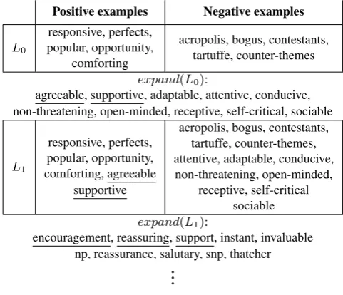
Figure 1: Example of the iterative term set expansion process. Starting out with an initial labeled term setL0consisting of five positive and five negative examples of the sought after term set, we expandL0to get ten candidate terms (expand(L0)). Of these ten candidate terms, the annotator labels “agreeable” and “sup-portive” as belonging to the sought after term set, and the labeled term set is updated accordingly. The procedure is then repeated with the updated term setL1, yielding ten new candidates which the annotator labels, and so on, until a satisfactory term set has been constructed. In this particular case, the sought after term set is the AFINN POS term set, with the “annotator” being a simple lookup as described in Equation 4. The performance of the term set expansion method would be the average number of positive examples added to the labeled term set, in this case2.5.

term set, i.e. with a labeling function defined as in Equation 4.

labelD(x) =

(

P ositive , x∈D

N egative , x6∈D (4)

Each combination of distributional model and expansion method was evaluated by running the term set expansion procedure for twenty steps, querying the “annotator” to la-bel ten candidate terms at each step, for ten random initial labeled term sets4_{. The reported performance is the average}

number of positive examples among the candidate terms per iteration. An example of the first step of this procedure can be seen in Figure 1: The initial labeled term setL0,

sam-ple from AFINN POS, is expanded, labeled, updated, and expanded again.

5. Results

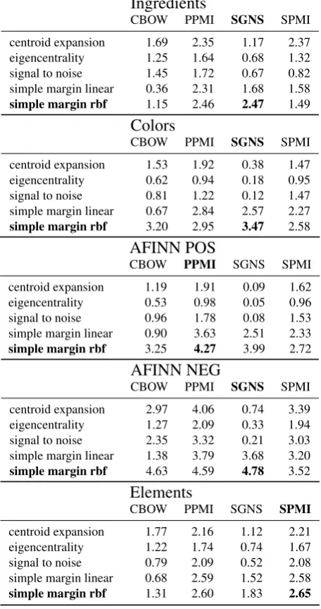
Table 1 shows the average performance as described in the previous section, i.e. the average number of positive ex-amples found per iteration. The results are displayed per tested term set, expansion method, and underlying distribu-tional model used. It is evident from this table that, gener-ally, Simple Margin using an RBF-kernel outperforms the other expansions methods. This is true for all term sets,

4

(4)

Ingredients

CBOW PPMI SGNS SPMI centroid expansion 1.69 2.35 1.17 2.37 eigencentrality 1.25 1.64 0.68 1.32 signal to noise 1.45 1.72 0.67 0.82 simple margin linear 0.36 2.31 1.68 1.58 simple margin rbf 1.15 2.46 2.47 1.49

Colors

AFINN POS

AFINN NEG

Elements

[image:4.595.56.284.75.507.2]

Table 1:Average number of positive examples found per iteration of the term set expansion method, based on ten random initializa-tion with five positive and five negative examples. Simple Margin using an RBF kernel is consistently the best expansion method for all term sets.

and almost all combinations of term sets and distributional models tested.

It is also evident that centroid expansion clearly outper-forms the other centrality based expansion methods, and in some instances, for some models, outperforms Simple Margin with a linear kernel.

6. Conclusion & discussion

As a best practice when using distributional methods for term set expansion, our results indicate that simple margin using an RBF-kernel is the best choice for all term sets, regardless of the distributional model used. Simple Mar-gin with a linear kernel – which has both the advantage of being directly representable in the vector space, and being efficient to compute – also consistently performed well for all distributional models but CBOW.

strong, enjoyed, excited, excellent, tremendously, thanks, marvellous, rich,disappointed, uplifting, fun, enjoy,

interesting, enjoying, healthy, terrific, lovely, ambitious, fantastic, enjoyable,worried, interested,sorry, improved, wonderfully, powerful,upset, successful, relieved, amazing,

Figure 2: Top 30 unlabeled candidates for AFINN POS using PPMI and Simple Margin with an RBF kernel after an expansion procedure as described in the section 4. The underlined words are those in the predefined term set, and the bold words are words that we deemed erroneous

It should be noted that, apart from providing the labeler with candidate terms, the simple margin methods also pro-vides a classifier based on the labeled set. This could be used to quickly expand the term sets – without supervision, but with some uncertainty – to include all terms the classi-fier would consider positive examples. An example of this can be seen in Figure 2.

Both SGNS and CBOW stands out: SGNS, while outper-forming most other models when using the RBF method, performed terribly in conjunction with centrality based methods. For CBOW, there is a significant loss of perfor-mance when using simple margin with a linear kernel, a phenomena not observed for the other distributional mod-els. This could indicate that the distributional representa-tions produced by SGNS are locally noisy but globally co-herent, and representations produced by CBOW are locally coherent, but globally noisy.

It should also be noted that the training data used for the dis-tributional models (BNC) is a comparably small, balanced, corpus. Results would be different for different sizes and kinds of corpora.

7. References

Clear, J. H. (1993). The digital word. chapter The British National Corpus, pages 163–187. MIT Press, Cam-bridge, MA, USA.

Eisenstein, J. (2017). Unsupervised learning for lexicon-based classification. In Proceedings of the Thirty-First AAAI Conference on Artificial Intelligence, February 4-9, 2017, San Francisco, California, USA., pages 3188– 3194.

Levy, O., Goldberg, Y., and Dagan, I. (2015). Improving distributional similarity with lessons learned from word embeddings. Transactions of the Association for Com-putational Linguistics, 3:211–225.

Mikolov, T., Sutskever, I., Chen, K., Corrado, G. S., and Dean, J. (2013). Distributed representations of words and phrases and their compositionality. In Proceedings of NIPS, pages 3111–3119.

Nielsen, F. ˚A. (2011). A new anew: Evaluation of a word list for sentiment analysis in microblogs. arXiv preprint arXiv:1103.2903.

Olsson, F. (2009). A literature survey of active machine learning in the context of natural language processing. Technical Report T2009:06.

(5)

International World Wide Web Conference, pages 161– 172, Brisbane, Australia.

Pantel, P., Crestan, E., Borkovsky, A., Popescu, A.-M., and Vyas, V. (2009). Web-scale distributional similarity and entity set expansion. In Proceedings of the 2009 Con-ference on Empirical Methods in Natural Language Pro-cessing: Volume 2-Volume 2, pages 938–947. Associa-tion for ComputaAssocia-tional Linguistics.

Sarmento, L., Jijkuon, V., de Rijke, M., and Oliveira, E. (2007). More like these: growing entity classes from seeds. InProceedings of the sixteenth ACM conference on Conference on information and knowledge manage-ment, pages 959–962. ACM.