The Phonon Thermodynamics of Iron and Cementite

(1)

Phonon thermodynamics of iron and cementite

Thesis by

Lisa Mary Mauger

In Partial Fulfillment of the Requirements for the Degree of

Doctor of Philosophy

California Institute of Technology Pasadena, California

2015

(2)

c 2015

(3)

(4)

Acknowledgments

This thesis was possible in no small part because of my adviser, Prof. Brent Fultz. It is with deep gratitude that I acknowledge all the help he provided me along the way. Brent was patient enough to let me explore various corners of our field, and watchful enough to reel me in when I drifted too far. I have learned to appreciate the deep wisdom in his comments and suggestions, even when they are too profound for my initial digestion. His direction, support and encouragement were essential to the work presented here, and I am extremely grateful for his guidance in shaping my scientific development. Perhaps most importantly, Brent has put together a fantastic team of budding scientists that I have been lucky enough to work with over the years.

(5)

Ahn, Michael McKerns, and John McCorquodale all dedicated their time to teaching me the ropes when I arrived. Mike Vondrus played a vital role, not only in machining the components we needed on my less than forgiving timelines, but also by providing design insight that greatly improved each project. I would also like to acknowledge the many administrative staff who are so vital to the interworkings of Caltech. Pamela Alberston gave me a thorough education on department history and protocals. Joan Sullivan helped our Keck laboratories weather the debris, noise, flooding and repairs that come with a sixty year old building. Christy Jenstad, our fantastic APh/MS option representative, who joyfully helped me navigate degree requirements while becoming a dear friend. I would like thank my thesis committee, for overseeing the final stages of my development here at Caltech – Prof. Jennifer Jackson, Prof. Bill Johnson, Prof. Dennis Kochmann, Prof. Austin Minnich and Prof. Keith Schwab, I appreciate the time and consideration you put into reading this document, and I look forward to thoughtful discussions yet to come. Prof. Jackson and Prof. Johnson have played especially important roles in the execution of this work, through valuable ongoing collaborations between our groups.

My graduate research provided me with opportunities to interact with wonderful scientists around the country and I greatly appreciate the time each of them took to train and mentor me. The staff of the Carnegie Institute of Washington were extremely important to my development as a scientist. They supported my research through the Carnegie - Department of Energy Alliance Center (CDAC), which provided a diverse scientific community with a wealth of experience and insight. I would like to specifically thank Dr. Steve Gramsch, Dr. Somayazulu and Dr. Russ Hemley for their support and collaboration. I would also like to thank the staff at the High Pressure Collaborative Access Team at Argonne National Lab. Their innovation and dedication has produced a unique and excellent facility. Dr. Yuming Xiao and Dr. Paul Chow provided countless hours of user support. Curtis Kenney-Benson and Eric Rod also played an essential role in making sure all the pieces fit together. My experimental achievements were built on the foundation provided by these dedicated scientists and engineers, and I remember our time together fondly. I would also like to acknowledge the staff of Sector 3 at the Advanced Photon Source for their support and contributions. Drs. Ercan Alp, Tom Tollner, Michael Hu, Jiyong Zhao and Wolfgang Sturhahn. The insight, support, dedication and humor lead to many productive beamtimes and other fun memories.

(6)

me forward - at school, in the gym, on the dance floor - greatly enriching my graduate experience. Finally I would like to acknowledge the unwaivering support of my boyfriend Chris, his appearance in my life has been a gift that I treasure.

(7)

Abstract

The vibrational properties of materials are essential to understanding material stability and thermo-dynamics. In this thesis I outline vibrational thermodynamic models and the experimental tools that provide evidence on phonon behavior. The introductory section discusses the history of metallurgy and thermodynamic theory, with an emphasis on the role of iron and cementite, two important com-ponents of steels. The thermodynamic framework for understanding vibrational material behavior is provided alongside the growing body of experimental and computational tools that provide physical insight on vibrational properties. The high temperature vibrational behavior of iron and cementite are explored within this context in the final chapters.

Body-centered-cubic iron exhibits decreasing phonon energies at elevated temperatures. The observed energy change is not uniform across phonon modes in iron, and specific phonon modes show significant decreases in energy that are not explained by simple vibrational models. This anomalous energy decrease is linked to the second-nearest-neighbor interactions in the bcc structure, through examination of fitted interatomic force constants. The large changes in phonon energy result in a significant increase in the vibrational entropy, called the nonharmonic vibrational entropy, which emulates the temperature behavior of the magnetic entropy across the Curie temperature. The nonharmonic vibrational entropy is attributed to interactions between the vibrations and state of magnetic disorder in the material, which persists above the magnetic transition and extends the stability region of the bcc phase.

Orthorombic cementite, Fe3C, exhibits anisotropic magneto-volume behavior in the

ferromag-netic phase including regions of very low thermal expansion. The phonon modes of cementite show anomalous temperature dependence, with low energy phonon modes increasing their energy at elevated temperatures in the ferromagnetic phase. This behavior is reversed after the magnetic tran-sition temperature and these same phonon modes lower their energies with temperature, consistent with observed thermal expansion. This atypical phonon behavior lowers the vibrational entropy of cementite up to the Curie temperature. The experimentally observed increase in low energy acoustic phonons affects the elastic behavior of Fe3C, increasing the isotropy of elastic response. First

(8)

(9)

List of Figures

1.1 Fe-C Phase Diagram . . . 2

1.2 Free energy of iron polymorphs . . . 4

2.1 Phonon Dispersions and Density of States forα-Fe . . . 10

3.1 Debye model for Fe thermodynamics . . . 14

3.2 Thermal expansion of Fe and Fe3C . . . 14

3.3 Quasi-Harmonic Debye model for Fe thermodynamics . . . 16

3.4 Temperature-dependentγT(T) forα-Fe . . . 17

3.5 Early thermodynamic assessment of Fe . . . 18

4.1 Mossbauer isomer shift and electric field gradient transition energies . . . 23

4.2 Mossbauer isomer shift and hyperfine magnetic field transition energies . . . 23

4.3 NFS Timing . . . 24

4.4 NRIXS Excitations . . . 26

4.5 NRIXS Spectra S(E) ofαFe . . . 27

4.6 Density of States (DOS) ofα-Fe . . . 28

5.1 Phonon Effects from 1NN Longitudinal . . . 34

5.2 Phonon Effects from 2NN Longitudinal . . . 34

5.3 Qualities of Fit for BvK DOS Test . . . 37

5.4 5NN Fits . . . 38

6.1 57_{Fe phonon DOS Spectra . . . .} ₄₄

6.2 57_{Fe phonon modes vs temperature . . . .} ₄₅

6.3 57_{Fe Entropy Contributions . . . .} ₄₆

6.4 DOS Fits and Dispersion Comparisons . . . 49

6.5 BvK Fitted Dispersions . . . 50

6.6 Thermal dispersion behavior divided by branch . . . 51

(12)

6.8 Thermal Behavior of High Symmetry Phonon Modes . . . 53

6.9 Nonharmonic Vibrational Entropy Comparison . . . 55

6.10 Nonharmonic Heat Capacity Contribution . . . 56

6.11 57_{Fe FCC Phonon DOS . . . .} ₅₈

6.12 Comparison of anharmonic phonon behavior with magnetic entropy . . . 62

6.13 Thermal behavior of Lamb-M¨ossbauer Factor . . . 62

7.1 The structure of Fe3C . . . 68

7.2 NRIXS phonon partial DOS of Fe3C . . . 70

7.3 Comparison of experimental and calculated phonon pDOS . . . 71

7.4 Mean phonon energy of the Fe pDOS . . . 72

7.5 Vibrational entropy of the Fe pDOS . . . 72

7.6 Sound velocities of Fe3C with temperature . . . 74

7.7 Comparison of NRIXS pDOS in the ferromagnetic and paramagentic phases . . . 75

7.8 Calculated phonon Fe pDOS at high temperatures . . . 77

7.9 Illustrations of phonons that stiffen with temperature at X and Z . . . 78

7.10 Illustrations of Y-point phonon modes . . . 79

7.11 Illustrations of Γ point low energy phonon modes . . . 79

7.12 Calculated Fe pDOS resolved onto distinct lattice sites . . . 80

7.13 Thermal trends of elastic modulie extracted from DFT . . . 83

(13)

List of Tables

5.1 Interatomic force constants of 300Kα-Fe . . . 33

6.1 The vibrational entropy ofα-Fe . . . 48

6.2 BvK Force Constants forα-Fe including 2NN . . . 60

6.3 BvK Force Constants forα-Fe including 4NN . . . 61

7.1 Fe3C experimental and computed lattice parameters . . . 68

7.2 Fe3C experimental and computer lattice sites . . . 69

7.3 Total Vibrational Entropy of Fe3C . . . 74

(14)

Chapter 1

Introduction

1.1

Iron and Steel - Ancient History

Great advances in human civilizations have come from the development of metalworking technol-ogy. However, early man lacked a sophisticated understanding of thermodynamics, so metalworking advances were based on carefully refined recipes rather than physical principles. Despite their lack of physical understanding, early man learned to isolate metals with heat and alloy substances to improve mechanical strength. These methodologies were largely dependent on the quality of raw materials and this knowledge was occasionally lost to time, only to be rediscovered generations later by different routes.

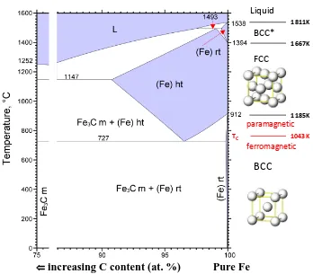
The discovery of iron and steels transformed civilizations, but this technology was hard won by early blacksmiths. While a steel composition can be as simple as iron with a few atomic percent carbon, the development of steel took centuries. We now understand that the mechanical benefits of steels that early man sought are enabled by the temperature-driven polymorphism in iron. The iron carbon phase diagram shown in Fig. 1.1 contains three thermodynamically stable regions of pure iron that form stable solid solutions with carbon. With increasing temperature pure iron transforms from a ferromagnetic bcc structure to a paramagnetic bcc structure (1043K) to a fcc structure (1185K) and then back to a bcc structure (1667K) before melting. This re-entrant temperature dependent polymorphism is not common among the elemental metals, and gives iron alloys a number of unique properties. The variability in mechanical properties of steels can be controlled to some extent by composition, but is more dramatically altered by metastable microstructure induced by controlled temperature cycling through the polymorphic transitions of iron.

(15)

Liquid

BCC*

1811K

FCC

1667K

BCC

ferromagnetic paramagnetic

⇐

increasing C content (at. %)

Pure Fe

1185K

[image:15.612.152.500.72.377.2]

TC 1043K

Figure 1.1: The Fe-C phase diagram, maps all stable phases with blue regions. This figure was constructed using the 1992 phase diagram developed by Okamoto, et. al. [1]. The phase regions labeled rt refer to the body-centered-cubic (bcc) solid solution phase, while the phase regions labeled ht refer to the face-centered-cubic (fcc) solid solution phase.

for early blacksmiths. Pure iron is also a relatively soft and ductile metal, which limited the early use of iron to small domestic applications. The discovery of steel occurred nearly 1000 years later, providing much greater strength and revolutionizing weaponry [2]. But producing quality steels was quite difficult for early man, who could not appreciate the thermodynamic forces driving his processes.

(16)

with temperature. But when the temperature of the iron carbon solid solution is lowered back to the body-centered-cubic phase stability range, the carbons have fewer favorable interstitial sites and attempt to diffuse out to form Fe3C shown on the left side of the phase diagram in Fig 1.1. However

if this diffusion limited process is interrupted, by rapidly lowering the temperature of the alloy, the carbon atoms get stuck in unpreferable interstitial sites and they distort they crystal structure locally, resulting in a significantly harder material called martensite.

This was the true birth of steels. The rapid quenching of hot Fe-C alloys in water can provide nearly a five fold increase in strength, making a product much harder than bronze, a Cu-Sn alloy, which was the technological standard of the time [2]. Once it was realized that the strength of steels could be adjusted by thermocycling alone, the technological potential was quickly realized. Today martensitic steels still provide the best strength per cost per unit volume of modern engineered materials [3].

1.2

The Dawn of Thermodynamics

The physical phenomena early man explored in manipulating metal alloys is now encompassed in the fields of modern thermodynamics and metallurgy. They refined ore into metals using heat in early furnaces. These metals were alloyed, heat treated, and worked by hand, adding a variety of properties to the components that are now understood to come from the atomic and microstructural arrangements these processes induced.

The efficient and effective processing of metals was a great driver of thermodynamic under-standing. Thus modern thermodynamics grew up beside the industrial revolution, when the old methodologies of metal working were traded for modern processes of great scale. The pioneering work of Josiah Willard Gibbs laid the groundwork for our modern understanding of phase diagrams and material equilibria [4]. Gibbs was a mathematician by training and focused on the geometries of early phase maps to draw connections between phase stability, energy and entropy. The Gibbs free energy,G,

G=H−T S (1.1)

is related to the enthalpy, H, temperature, T, and entropy, S, of a substance in a given state. The early work of Gibbs emphasized the generality of thermodynamic principles to include material systems of all kinds [4]. His pioneering insights slowly brought scientific unity to the practices of chemical metallurgy, by uncovering the underlying principles in the centuries of collected physical observations and material preparation methodologies.

(17)

low temperature heat capacity behavior [6]. This laid the groundwork for physical interpretations of observed thermodynamic properties in solids.

It was quickly understood that the unique polymorphism of iron provided for the great diversity of technological properties of iron-based alloys. Improving iron-based steels was of intense industrial interest, and thus improved thermodynamic understandings were readily applied to iron alloys. Improvements in calorimetry around the same time produced experimental measures of free energy derivatives. Attempts to quantify the free energies driving the diverse microstructures of steels quickly followed. An early assessment of the free energies of iron was provided by Austin as shown in Fig. [7].

[image:17.612.218.429.243.495.2]

bcc

f

cc

bcc

Figure 1.2: The free energy of bcc (α-Fe) and fcc (γ-Fe) extracted from calorimetry measurements [7].

This was the beginning of physical metallurgy, where detailed methodologies could finally be understood in terms of physical consequence. The chemical consequences of iron’s polymorphic phase transitions were mapped on phase diagrams where thermodynamic insight was used to ex-plore new compositions. The equilibrium positions of carbon in iron changes substantially with crystal structure, and cementite or Fe3C will precipitate for many compositions at modest

(18)

steel-metallurgy.

Structural steels weren’t the only technological materials to highlight the interesting physical behavior of Fe during the industrial revolution. The unique physical properties of Fe also participate in materials that are famous for something other than their strength. The 1920 Nobel prize in physics was awarded to Charles Guillaume “in recognition of the service he has rendered to precision measurements in physics by his discovery of anomalies in nickel steel alloys” [8]. The anomaly that so captivated the Nobel committee was a thermo-volume behavior of FeNi alloys resulting in a near vanishing thermal expansion for a wide temperature range at a specific composition. The Fe64Ni36

(19)

Chapter 2

Crystals and Phonons

2.1

Crystal Lattices

Both the models of Einstein and Debye relied on the notion of crystalline solids. Which was verified by the early work of W. H. and W. L. Bragg [9]. The x-ray pattern observed with Bragg diffraction is the result of regularly repeating arrays of atoms in crystalline materials. The arrangement of the atoms in a crystal can be reduced to a set of translational symmetry operations that relate every atomic position in a perfect crystal onto all equivalent positions, thus defining the lattice symmetry of crystalline solids, and simplifying their structure to a primitive unit cell that may be tessellated to map out every lattice position. One may then define lattice translation vectors,r, as

r=x1a1+x2a2+x3a3, (2.1)

wherexjare integers anda1,a2, anda3are the primitive lattice translation vectors, wherea1·a2×a3

defines the primitive unit cell volume. A reciprocal lattice can then be defined for each type of lattice, based on the constraints of Bragg’s law, which observed the relationship between the wavevector of the incoming radiation and the structure of the crystal lattice. The reciprocal lattice has a complementary set of vectors,q, defined as

q=y1b1+y2b2+y3b3, (2.2)

where the prefactorsyi are again integers andb1,b2,b3 are defined as the primitive vectors of the

reciprocal lattice. These special reciprocal space vectors (also referred to here asq-space vectors) can be constructed from the real space lattice vectors as

b1= 2π

a2×a3 a1·a2×a3

,b2= 2π

a3×a1 a1·a2×a3

,b3= 2π

a1×a2 a1·a2×a3

. (2.3)

(20)

The principles of lattice symmetry discussed here can easily be extended to include compounds with multiple atomic species. In this case the primitive unit cell is still the smallest volume that can be tessilated to map all space, defined by three primitive lattice vectors. The only distinction is that the lattice has a basis, which is typically described by vectors that connect the positions of unique atoms in the primitive cell. It is within this symmetry that we can now begin to define the lattice modes, or quanta of vibrations called phonons [10].

2.2

Phonons

The equilibrium interatomic distances offer an energy efficient packing that optimizes the interactions of the atomic electrons. The positions geometrically optimize the interatomic forces to set the equilibrium distances. We will describe this potential energy of the interatomic interaction asφ(R), whereRis the distance between a pair of atoms. The potential energy of a crystal,U, can then be described by summing over all the pairs of atoms in a crystal,

U = 1

2 X

i,j

φ(ri−rj). (2.4)

If an atom indexed by i is perturbed a small distance from its equilibrium position, ri, to a new

position, ri+ui, the neighboring unperturbed atoms would exert a force on the displaced atom

to return it to its equilibrium position. A Taylor expansion of the potential energy U for small displacements of the atoms,ui, from their equilibrium positions gives

U = 1

2 X

i,j

φ(ri−rj) +

1 2

X

i,j

(ui−uj)· ∇φ(ri−rj) +

1 4

X

i,j

[(ui−uj)· ∇]2φ(ri−rj) +O(u3i). (2.5)

Here the first term is the constant equilibrium crystal potential, the linear second term is the restoring forces that sum to zero over the crystal, and the remaining term is the harmonic term of the original potentialφ(R), which can be written as

Uh= 1 4

X

i,j&µ,ν=x,y,z

(ri−rj)µ

∂2_φ₍_r i−rj)

∂(ri−rj)µ∂(ri−rj)ν

(ri−rj)ν. (2.6)

This simplification is called the harmonic approximation because it neglects higher order terms in the potential. The gradient term at the heart of this expression gives the force constant between two atoms in a specific Cartesian direction. This expression can be generalized by defining a force constant matrix, K, that encompasses all the atomic interactions represented in the derivatives of

φ:

Uh= 1 2

X

i,j

(21)

With the proper symmetry constraints and Born-von K´arm´an periodic boundary conditions, we cleverly select a general description of the displacements that is appropriate for translational symmetry:

ui(t) =ei(k·ri−ωt), (2.8)

where is the polarization of the atomic displacement in Cartesian coordinates. We can solve for the equations of motion given our harmonic potential, where

Mu¨i=−

∂Uh

∂ui

=−X

j

K(ri−rj)uj. (2.9)

Our system of N atoms has 3N discrete vibrational modes that can be supported by the crystal, and our equation of motion becomes

M ω2=X

j

K(rj)e−ik·rj=D(k). (2.10)

This expression is called the dynamical matrix expression, where D(k) is the dynamical matrix. The dynamical matrix contains the force constants (or potential derivatives) for every pair of atomic interactions in the crystal. For an atom in a real crystal we know that the largest contribution to the restoring forces will come from the atoms immediately around it, so we can truncate the dynamical matrix to include only the most pertinent nearest-neighbor restoring forces, often without a significant loss of accuracy. The dynamical matrix expression can be solved for the normal mode frequenciesωand mode wavevectorsat everykin reciprocal space.

This methodology connects the symmetry of the lattice with the allowed normal modes and the interatomic forces driving them; however, quantum mechanical considerations are required to extend this description of lattice modes to quantized vibrational excitations called “phonons”. These considerations ensure that vibrations are properly counted a low temperatures, where their discrete nature becomes apparent. The energy of a crystal is described by 3N quantum harmonic oscillators with frequencies from the dynamical matrix expression, but governed by Bose-Einstein occupation statistics. Thus the Hamiltonian for a crystal transitions from its classical definition,

H = 1

2M

X

i Pi2+

1 2

X

i,j

uiD(ri−rj)uj (2.11)

to its quantum representation,

H=X

k,s

¯

hωs(k)(α†ksαks+

1 2) =

X

k,s

(nks+

1

(22)

where the phonon creation operatorα†_k_sand phonon annihilation operatorαks are defined as

α†_k_s=√1

N

X

i

e−ik·ri

s(k)

"r

M ωs(k)

2¯h ui−i

s 1 2¯hM ωs(k)

pi

#

(2.13)

and

αks=

1 √

N

X

i

e−ik·ri

s(k)

"r

M ωs(k)

2¯h ui+i

s 1 2¯hM ωs(k)

pi

#

(2.14)

and

nks= (e

¯ hωs(k)

kB T ₋₁₎−1_. _(2.15)

The important distinction between these two models is readily observed in experimental heat capac-ities. The heat capacity,C, is the temperature derivative of the internal energy of a material,U. In the classical harmonic oscillator formalism,U(T) is a linear function ofT, so the heat capacity

C=∂U

∂T =

∂ ∂T(U

eq_{+ 3}_{N k}

BT) = 3N kB (2.16)

is constant for all temperatures. However, the heat capacity of a set of quantum harmonic oscillators contains a temperature-specific term

C=∂U

∂T =

∂ ∂T(U

eq

+X

ks

(nks+

1

2)¯hωs(k)) = X

ks

∂

∂T(nks)¯hωs(k) =

X

ks

∂ ∂T

¯

hωs(k)

e

¯ hωs(k)

kB T ₋₁

, (2.17)

which recovers the experimentally-observed temperature dependence of the heat capacity at very low temperatures. Using quantum harmonic oscillator formalism in the calculation of lattice ther-modynamic variables will include the zero-point vibrational energy of the solid [11].

2.3

Observations of Phonons

(23)

[image:23.612.112.534.98.311.2]

en-ergy. These points are then analyzed with the harmonic model developed in the previous section.

Figure 2.1: Phonon dispersions from triple-axis inelastic neutron scatter (points), overlaid with Born-von K´arm´an model fits and the resulting phonon density of states shown on the right [12].

The phonon dispersion points are fit to force constants in a dynamical matrix, typically using a least squares optimization that seeks to minimize the system of equations against all the observed phonon measurements. This requires truncating the dynamical matrix to a subset of all the interactions in the material, typically limiting restoring forces to the closest neighboring atoms. Minkewicz utilized the atomic interactions for the first through fifth nearest neighbors, obtaining the fits shown in Fig. 2.1. The force constants can be used to describe phonon behavior in other portions of q-space where measurements were not collected. They can also be integrated over all of q-space to provide a phonon density of states (DOS), which is also shown in Fig. 2.1. The phonon density of states can be readily used to describe the phonon thermodynamics of materials.

(24)

(25)

Chapter 3

Thermodynamics

3.1

Thermodynamic Relations

Thermodynamics was useful to 20th century metallurgists insofar as it can be used to predict and extrapolate properties beyond those directly measured. A functional thermodynamic understanding of iron was readily applied to understanding the technologically-relevant properties of iron alloys.

The Gibbs free energy of a solid, G, can be divided into enthalpy and entropy terms. Under constant volume conditions, the enthalpy of a solid,H, is largely determined by the internal energy,

U, which can be characterized as the energy involved in assembling a set of atoms into their solid configuration. The entropy of a solid,S, enumerates the way heat is stored in a material. Both en-thalpy and entropy can be extracted by integrating the measured heat capacity at constant pressure,

CPusing the expressions

H(T) = Z T

0

CP(T0)dT0 (3.1)

and

S(T) = Z T

0

CP(T0)

T0 dT

0_. _(3.2)

In solids at finite temperatures (above ambient conditions) the free energy contribution from en-tropy,T S, changes more rapidly than the enthalpy, H, dominating the thermal effects on the free energy. For ordered crystalline solids, lattice vibrations make the largest entropic contribution,Svib.

Electronic excitations also create entropy,Selec, though noticeably smaller than vibrational entropy.

Solids that exhibit magnetic ordering will also have magnetic excitations that perturb spins from their ground state orientation, providing magnetic entropy,Smag. These three contributions,

vibra-tional, electronic, and magnetic excitations, enumerate the ways that heat can be stored in iron and comprise its entropy. These contributions are hoped to be adiabatically separable, providing the expression

(26)

Understanding the entropy of a solid will greatly inform the temperature-dependent behavior of its free energy, which is essential to developing the theoretical basis for high temperature phase diagrams. Early thermodynamic research sought to reconcile these physical excitations with the aggregate thermodynamics that drives phase transitions. Experimental heat capacities provided a basis for comparing observed thermodynamic properties with theoretical models. But direct mea-surement of the phonon density of states of a material can also provide complementary information that may be used to assess the phonon-specific contributions to thermodynamics.

The phonon contribution to the entropy,Svib, may be calculated directly from the phonon DOS,

g(E), at the temperature that the phonon DOS was acquired

Svib(T) = 3kB

Z

gT(E){(n+ 1) ln(n+ 1)−nln(n)}dE. (3.4)

Where the integral goes over all phonon energies, and the Planck functionnis a function of energy and temperature only, simplified from Eqn 2.15 to n = (ekB TE ₋₁₎−1_{. Additionally the phonon} contribution to the heat capacity,Cvib

p , may be calculated from the phonon density of states,

C_pvib= 3

kB

Z _∂n

∂TgT(E)EdE. (3.5)

These expressions provide another route to the thermodynamic behavior of materials that focuses on the phonon contributions alone, by using the phonon density of states. Since the phonon con-tribution to thermodynamics is almost always the largest thermodynamic concon-tribution at finite temperatures, early thermodynamic models focused on quantifying the phonon behavior through various formalisms.

3.2

Debye Model

The Debye model for the vibrational response of the solid makes use of the quantum mechanical nature of phonons, but largely ignores the details of how phonons relate to the symmetry of the structure. Debye simplified the normal mode relationships of a crystal considerably by assuming that the phonon frequencies ω obeyed a linear relationship with respect to the reciprocal lattice vector,k,ω=c|k|, wherecis the sound velocity of the phonon. The assumption of linear phonon branches only applies rigorously in the long wavelength limit (at very low |k|). The complicated mathematical formulations of the previous section are simplified to three isotropic acoustic phonon branches. By selecting an isotropic cutoff for the outer limit of reciprocal space, kD = 3

p 6π2_ρ_,

(27)

The identical linear isotropic acoustic branches can be integrated over the spherical Brillioun zone to provide a phonon density of states, which enumerates the available phonon modes in the crystal by their energy level. The Debye heat capacity and phonon density of states are plotted in Fig. 3.1 for ΘD= 420, which is the Debye temperature commonly used forα-Fe.

QD=420

0 10 20 30 40 50

0.00

0.02

0.04

0.06

0.08

EnergyHmeVL

DOS H 1 meV L

CpHtotL

CPHhL

0 200 400 600 800 10001200 0 2 4 6 8 10

TemperatureHKL

Cp

H

kB

atom

L STotal

SvibHhL

0 200 400 600 800 10001200 0 2 4 6 8 10

TemperatureHKL Svib H kB atom L

Figure 3.1: Debye model phonon density of state for ΘD= 420, a typical value used for α-Fe [19].

The corresponding vibrational heat capacity compared with α-Fe experimental heat capacity [20]. The Debye vibrational entropy compared with the total entropy of α-Fe from the SGTE database [21]

The heat capacity derived from the Debye model is capable of reproducing both the empirical Dulong-Petit high temperature limit, and also the low temperatureT3behavior observed in measured heat capacities. The Debye temperature is commonly determined by fitting to low temperature heat capacity data. Once a Debye temperature is obtained, the full vibrational thermodynamics of a crystalline solid are mathematically accessible. This model is, however, a strictly harmonic approach, which is often too simple for the behavior of the phonon modes in real crystals. The harmonic formalism fails to explain natural phenomena like thermal expansion of solids and thermal resistivity of materials. These effect arise from other interactions that are truncated in our expression for the interatomic potential. The inability of the Debye model to deal with the physical effects of thermal expansion led to several modifications that are called “quasi-harmonic” models.

Α-Fe Γ-Fe ∆

TC

0 500 1000 1500

23.5 24.0 24.5 25.0 25.5

TemperatureHKL

Volume

H

Å

3L

also strongly temperature dependent, at least for the temperature interval covered in this experiment. Similar behaviour is observed, for example, in-iron (Kohlhaaset al., 1967), associated with the ferromagnetic phase transition at about 1045 K. This competition between the thermal expan-sion arising from vibrations of the atoms and the increase in volume with decreasing temperature arising from spontaneous magnetostriction provides the basis for the family of `Invar' alloys (such as Fe with 36 wt% Ni), which have very low thermal expansion around room temperature.

Current studies of Fe3C are mainly concerned with its

possible occurrence in the Earth's core; it is, therefore, its physical properties in a high-pressure `non-magnetic' state (with Pauli paramagnetism but in which there are no local magnetic moments on the atoms) that are of most interest to Earth scientists. Such a phase only exists above 60 GPa (VocÏadlo, Brodholtet al., 2002) and is therefore not readily accessible experimentally. The accessible high-temperature paramagnetic phase (in which there are local magnetic moments but they are randomly disordered) will, however, be more representative of the core-forming phase than the ferromagnetically ordered material (for further discussion see below). To determine the thermal expansion coef®cient of this phase in the form tabulated by Fei (1995), the eight data points shown in Fig. 2 for whichT460 K were ®tted to

VT VTrexp

RT

T_r TdT

" #

; 1

whereVTris the volume at a chosen reference temperature,Tr, and(T) is the thermal expansion coef®cient, having the form

T aoa1T: 2

This ®t gave values of VTr = 154.8 (1) AÊ 3_, _a

o = ÿ4 (2)

10ÿ5_Kÿ1_and_a

1= 1.6 (3)10ÿ7Kÿ2, for a chosenTrof 300 K.

The large standard uncertainties inaoanda1arise from the

limited temperature range and the small number of data points available. The form of these parameters, with ao

negative and a1 strongly positive, re¯ects the strong

temperature dependence ofseen in the data, but probably also implies that it would be unwise to use them to extrapolate

to much higher temperatures. Expressed in this way,takes values of 3 (2)10ÿ5_Kÿ1_{at 460 K and 6 (3)}₁₀ÿ5_Kÿ1_at

600 K, in good agreement with the results of Reed & Root (1998) from which a temperature-independent value of 5.2 (2)

10ÿ5_Kÿ1_{can be derived [de®ned as}_{= (1/}_V_)(d_V_/d_T_)].

J. Appl. Cryst.(2004).37, 82±90 I. G. Woodet al. Cementite 85

research papers

Figure 3

(a) Unit-cell volume of Fe3C as a function of temperature. The symbols

show the measured data points (the estimated standard uncertainties lie within the symbols). The line shows the results of the ®t to equation (4).

(b) Volumetric thermal expansion coef®cient of Fe3C as a function of

temperature. The symbols were obtained by numerical differentiation of

the data shown in (a). The line was obtainedviaequation (4).

Figure 2

Lattice parameters of Fe3C as a function of temperature; the error bars

shown are at1 the estimated standard uncertainty.

(28)

3.3

Quasi-Harmonic Models

Quasi-harmonic models attempt to rectify the shortcomings of the harmonic models by taking into account the effects of thermal expansion. In a strictly harmonic model, the vibrational degrees of freedom have no dependence on the volume of a solid or its temperature. In 1926, Eduard Gr¨uneisen proposed a thermodynamic equation of state for matter that incorporates the vibrational effects from changes in volume at finite temperatures. He defined the phonon mode Gr¨uneisen parameter,γj,

γj=−

∂lnωj

∂lnV |T ' − V ωj

∆ωj

∆V , (3.6)

a unitless scaling parameter defined in terms of the phonon frequency, ωj, and the volume, V,

of the solid [24]. Gr¨uneisen used this description to develop a thermodynamic equation of state which incorporates quantum mechanical lattice contributions. However experimental data onγj for

individual phonons is extremely rare.

More often an average bulk Gr¨uneisen parameter γT is constructed to model the bulk material

behavior

γT =V

∂P ∂U|V =

αKT

CVρ

(3.7)

where V is the volume, P is pressure, α is the thermal volume expansion, KT is the isothermal

bulk modulus,CV is the heat capacity at constant volume, andρis the atomic density [24]. While

the microscopic Gr¨uneisen parameter, γj, is an exact thermodynamic definition, models that use

the thermal Gr¨uneisen parameter,γT, often include approximations such as an isotropic crystalline

response. However,γT can be readily obtained from ambient measured bulk properties of a material,

yielding values typically lie between 1 and 2 for most well-behaved materials [24]. The thermal Gr¨uneisen parameter forα-Fe is 1.81 [24], and the thermal Gr¨uneisen parameter for Fe3C is between

2.0 and 2.4 depending on which values for the bulk modulus you trust. ThisγT can then be used in

the microscopic definition to scale observed phonon frequencies with temperature

ω(T) =ω0(1−γT

V −V0

V0

). (3.8)

If the Debye model provides the phonon DOS, then the Debye DOS can be scaled with thermal expansion to provide the QH vibrational entropy of a material. However, the Debye DOS can readily be replaced with an experimentally determined phonon density of states without altering the nature of the model. A quasi-harmonic model that utilizes an average thermalγT has no frequency

dependence; all phonons shift in energy the same way. The effect of the quasi-harmonic model is completely independent of the vibrational spectra being scaled.

(29)

energy) can be ascertained by calculating the heat capacity and the vibrational entropy from the en-ergy shifted phonon DOS. The quasi-harmonic vibrational entropy can be calculated using Eqn. 3.4, and the heat capacity can be calculated using Eqn. 3.5. Under the quasiharmonic approximation the heat capacity can also be re-written to directly include thermal expansion using a Gr¨uneisen parameter without using the phonon DOS. This expression is called the Nerst-Gr¨uneisen expression,

CP =CV(1 + 3γTα(T)T), (3.9)

where α(T) is the linear thermal expansion. The thermodynamic contributions from the quasi-harmonic model are compared with the quasi-harmonic Debye model curves of the previous section in Fig. 3.3.

ΓTHTL

Γ = ΓTH300L

0 200 400 600 800 1000 0.92

0.94 0.96 0.98 1.00

TemperatureHKL

ΩQHA

Ω0 CpHtotL

CPHqhL

CPHhL

0 200 400 600 800 10001200 0 2 4 6 8 10

TemperatureHKL

Cp

H

kB

atom

L STotal

SvibHqhL

SvibHhL

0 200 400 600 800 10001200 0 2 4 6 8 10

TemperatureHKL Svib H kB atom L

Figure 3.3: Debye model phonon density of state for ΘD= 420, a typical value used for α-Fe [19].

The corresponding vibrational heat capacity compared with α-Fe experimental heat capacity [20]. The Debye vibrational entropy compared with the total entropy of α-Fe from the SGTE database [21].

High temperature calculations with the QHA often employ a constant Grüneisen parameter, though the bulk thermal properties encompassed in the thermal Grüneisen parameter have been observed to vary with temperature in a number of materials. In an attempt to rectify this problem, a temperature-dependent Grüneisen parameter can be used. For the case of pure iron, a wealth of information on temperature-dependent properties is available. Multiple assessments of temperature dependent thermal expansion [22, 25–27] and bulk modulus [28–30] can be used. The heat capacity at constant volume,CV, can also be calculated in a number of ways with different approximations.

We examined the temperature dependence of the Gr¨uneisen parameter by constructing two separate functions forγT(T) that sampled the full range of observed values in the literature. The

results of these assessments are shown in Fig. 3.4, and show variations in γT(T) between 1.5 and

2.1 over the temperature range of interest. Phonon frequencies can be scaled according to the temperature-dependent Gr¨uneisen parameter using the following expression:

ω(T) =ω0 Ti=T

Y

Ti=1

[1−γT(Ti)(

V(Ti)

V(Ti−1)

(30)

Γ

_T

H

T

L

: K

T

-

Rayne

Dever

Α-

TPRC, C

v

-

Debye,

Ρ-

TPRC

Γ

T

H

T

L

: K

T

-

Adams

Dever

Α-

Liu, C

v

-

NRIXS,

Ρ-

Seki

0

200

400

600

800

1000

1200

1.5

2.0

2.5

Temperature

H

K

L

Γ

T

H

T

[image:30.612.184.468.71.268.2]

L

Figure 3.4: The temperature-dependent Gr¨uneisen parameterγT(T) assembled from various

litera-ture values. BlackγT(T) fromKT[28, 30],α[22],CV from a Debye model (ΘD=420K), andρ[22].

RedγT(T) fromKT [28, 29],α[25],CVfrom 14K NRIXS measurements, and ρ[26].

which reduces to Eqn 3.8 whenγT is a constant. The result of this more careful calculation was nearly

the same as calculated quasi-harmonic change in frequency for a constantγT =γT(300K), as shown

in the left panel of Fig. 3.3. The resulting changes in the vibrational entropy from includingγT(T)

were always below 0.5% at 1180K. Therefore, in the case of bcc iron, the addition of a temperature-dependent Gr¨uneisen parameter has only a small effect on the calculated phonon energies. The temperature dependence is influenced much more by the selected thermal expansion values.

(31)

Phonons Electrons Magnons

400 600 800 1000 1200

0 200 400 600 800

TemperatureHKL

H

meV

atom

L

Phonons Electrons Magnons

400 600 800 1000 1200

-800 -600 -400 -200 0

TemperatureHKL

TS

H

meV

atom

L

Figure 3.5: The enthalpic and entropic contributions to free energy [19].

and captures only aggregate vibrational behavior. His assumption that magnetic entropy must be the remaining unassigned entropy points out a shortcoming that has long thwarted thermodynamic assessments of magnetic materials. Few models exist that can accurately describe finite temperature magnetic disorder, and there are even fewer experimental studies for comparison. The state of spin disorder in magnetic materials at finite temperatures remains an active field of study today [31].

3.4

Anharmonic Effects

The harmonic approximation of the interatomic potential simplifies many aspects of the physics of vibrations, and this approximation is normally valid for low temperatures. However there are several important physical phenomena that cannot be resolved by harmonic descriptions. The harmonic model assumes that phonons are quantum harmonic oscillators, which are non-interacting. However, we know that phonons do interact in real systems; phonons may interact with each other and also with other excitations that occur in real materials. Thermal expansion is the most obvious anharmonic thermal effect, and while the quasi-harmonic approximation may improve the accuracy of thermodynamic models to deal with observed thermal expansion – it is by no means a physically rigorous approach. Nonharmonic interactions also result in routinely-observed phenomena like finite thermal conductivities, which result from phonon scattering events that indicate real phonons have finite lifetimes. Phonons are also known to play a role in electrical resistivity, where electronic carriers scatter, creating phonons that can increase the temperature of a material.

(32)

three new phonons, or two phonons interacting to create two new phonon states. These processes are governed by the laws of energy and momentum conservation. Thus not all combinations are possible; new states must have the proper energy and momenta, which are governed by the allowed crystal modes and described by the phonon dispersions. While the probability of multiphonon processes are low at low temperatures, they do have appreciable effects at finite temperatures when large phonon populations are present in the material.

In perturbation theory, it is often possible to keep only the next highest order term to improve on the physical description. While this could be done with the interionic potential, there are many physical arguments for keeping both the cubic and quartic term. The cubic term is asymmetric in nature, creating physical situations where the potential may become unstable if only this term is applied. There are also many crystalline symmetry constraints on the phonon processes produced by the cubic interaction term that limits the number of anharmonic interactions that are described by this formalism. Incorporation of the quartic term improves the limiting behavior of the net potential (since a Hamiltonian retaining only the cubic term may be unstable) [11]. Further, ob-servations of high temperature phonon behavior suggest that in many instances quartic interactions may contribute comparable thermodynamic effects to those from cubic term interactions.

Experimental characterizations of phonons in materials at high temperatures can begin to quan-tify the importance of these effects. Anharmonic phonon-phonon interactions affect the observed phonon spectra by both shifting their absolute energies, and also broadening their energy and q-space signatures. This is apparent in measurements of phonon dispersions and DOS measurements when the thermal broadening of specific features overcomes the instrument resolution, resulting in a broadening that scales with temperature. In high temperature phonon measurements of bcc Ti, Zr, and Hf, very broad phonon signatures have been resolved in specific q-space directions. This anomalously large broadening extends over a significant energy range and has been implicated as a dynamic precursor of the first-order martensitic transformation between the bcc and hexagonal crystal structures [32–34].

The anharmonic phonon broadening caused by more typical cubic and quartic interactions are expected to be Lorentzian in nature [35]. In phonon DOS measurements the anharmonic broadening of DOS features can be modeled using a modified Lorentzian function [14, 36]. This construction provides a route for estimating mean phonon lifetimes from spectra broadenings. Results from investigations of relatively isotropic elemental metals have shown that anharmonic effects are often linear with temperature.

(33)

(34)

Chapter 4

Experimental Methods

4.1

The M¨

ossbauer Effect

Rudolf Mössbauer won the 1961 Nobel Prize in Physics for “his researches concerning the resonance absorption of gamma radiation and his discovery in this connection of the effect which bears his name” [8]. Theeffect which bears his name is the recoilless nuclear resonance absorption of gamma rays by nuclei. The concept of resonant nuclear absorption and flourescence preceded Mössbauer’s initial work; however, the phenomena had not been observed efficiently because it was argued that the nuclear recoil should alter the energy of the photon emitted from the decay of the nuclear excited state. When Mössbauer observed this phenomena in 1958 he realized that recoilless nuclear resonant absorption was possible because the recoil was not confined to a single nucleus, but rather the entire crystal in which that atom was embedded. The recoil momentum is taken up by the entire crystal, whose mass is much much greater than a single nucleus, and accordingly the energy shift associated with the recoil upon gamma ray emission is negligibly small [37]. The efficient nuclear resonance comes from a finite probability that the energy transferred to the crystal lattice during a nuclear decay occurs without the excitation of a vibration in the lattice. These processes produce gamma rays capable of re-exciting other resonant nuclei in the lattice. There are many nuclei that exhibit recoil-free resonance, but the ease of which a nuclear excitation can be induced and observed have limited Mossbauer spectroscopy to a few more practical isotopes.

(35)

absorption of resonant nuclei. The small energy alterations from hyperfine interactions produce unique signals in Mössbauer spectroscopy about the local electronic environment of the resonant nucleus. To date the Mössbauer effect has been demonstrated on more than 100 different isotopes, but only a few are practical with conventional Mössbauer spectroscopy [38]. Rudolf Mössbauer’s original work used the 191 isotope of iridium, but today57_{Fe is the most commonly used isotope for}

Mössbauer spectroscopy. The ubiquity of iron in many geological, technological, and biological ma-terials makes57Fe Mössbauer spectroscopy the most commonly employed nuclear resonant isotope. Natural iron contains about 2% of the 57Fe isotope, which is sufficient for many studies of natural materials. This thesis work is on iron alloys, so the following discussion of Mössbauer spectra will focus on the57_{Fe nuclear excitations.}

M¨ossbauer spectroscopy utilizes a Doppler shift to sweep through energies around the nuclear resonant energy. Depending on the local environment of the nuclei, a number of hyperfine interac-tions can be identified in the spectra. These features appear as the splitting of the nuclear resonant energy levels as a result of the local electronic environment at the nucleus. In addition to the recoil free fraction, the number of nuclear excitations that produce a resonant recoil-free gamma ray, there are three other quantities that are commonly measured with M¨ossbauer spectroscopy. These three quantities are from the hyperfine interactions, and their schematic effects on the resonant nucleus are illustrated in Fig. 4.1 and Fig. 4.2.

The isomer shift is a hyperfine interaction that is present in every M¨ossbauer spectrum. The isomer shift is a measure of the electron density in the nucleus. It arises from size differences between of the nuclear excited state and the ground state, which interact with the electron wave function at the nucleus. The isomer shift results in a small change of the nuclear resonant excitation energy as shown in Fig. 4.1. In the absence of other hyperfine effects, the isomer shift can be used to track changes in occupation of the s-electronic states that have finite density at the nucleus.

The electric quadrupole splitting is another hyperfine interaction observed in the M¨ossbauer spectra of many materials. This effect splits the excited state of the nucleus as part of an interaction with the electric field gradient at the nuclear position. The electric quadrupole splitting arises from the electric quadrupole moment of the nucleus, which has a different orientation in the nuclear ground and excited states. In the presence of an electric field gradient, which occur at crystal sites with less than cubic symmetry, the nuclear resonant feature in the spectra is split symmetrically about the centroid dictated by the isomer shift.

(36)

In = ± 3/2

In= ± 1/2

∆E 57_{Fe =}

14.41 keV

Isolated

Nucleus Isomer Shift

In = ± 3/2

I_n= ± 1/2 In = ± 1/2

Electric Field

Gradient

[image:36.612.191.461.84.259.2]

∆E ~ neV

Figure 4.1: Changes in the nuclear excitation that correspond with an isomer shift and an electric field gradient.

In = ± 3/2

In= ± 1/2

∆E 57Fe = 14.41 keV

Isolated

Nucleus Isomer Shift

In = - 1/2

In = + 1/2

Hyperfine Magnetic Field

∆E ~ neV

In = + 1/2

In = - 1/2

In = + 3/2

In = - 3/2

∆E ~ neV

Figure 4.2: Changes in the nuclear excitation that correspond with an isomer shift and a hyperfine magnetic field.

magnetic field at the nucleus.

The hyperfine interactions of many resonant isotopes in different materials have been thoroughly studied throughout the years, providing a near fingerprint recognition quality to this method. The method is routinely used to characterize the different atomic environments present in both natural and engineered materials. There is a57_{Fe M¨}_{ossbauer spectrometer on the Mars rover [39].}

[image:36.612.154.497.321.515.2]

(37)

4.1.1

Nuclear Forward Scattering

New high-brilliance synchrotron sources enable a different approach to M¨ossbauer spectrometry. The synchrotron offers a new way to excite resonant nuclei without radioactive sources. Ruby first proposed this experimental arrangement in 1974 [42], though it was several years before synchrotron M¨ossbauer spectroscopy (SMS), also known as nuclear forward scattering (NFS), was realized exper-imentally. In addition to the high flux of third-generation synchrotron sources in the energy range of several resonant nuclei, single crystal silicon monochromators played an important role in the technique by refining the incoming x-ray spectrum [43].

The incoming synchrotron pulse interacts with the resonant nuclei, producing a coherent beam in the forward direction that is modulated by the hyperfine splittings of the nuclear resonant states [44](Smirnov for more detail). Unlike conventional M¨ossbauer spectrometry, which relies on a con-tinuous photon signal modulated in energy, SMS uses a temporally-resolved photon pulse to excite the nuclei. The synchrotron pulse arriving at the sample excites both the nuclear resonance and many other atomic excitations. However the relatively long lifetime of the nuclear excited state makes it possible to make high fidelity measurements of the temporal dependence of nuclear decays long after electronic processes have abated. This effect is shown schematically in Fig. 4.3. This

0 153 306

Time Delay (ns)

Log

[In

te

ns

ity

[image:37.612.111.539.384.484.2]

]

Figure 4.3: Synchrotron pulses arrive separated by 153ns. The signal from electronic excitations (blue) occurs within a new nanosecond, while the signal from nuclear resonant excitations (orange) can be monitored between pulses, when the background signal from other processes is extremely low.

measurement technique is enabled by the synchrotron timing structure, which produces short pulses of radiation followed by relatively long periods where no radiation arrives. When NFS spectra are collected, the detector is gated electronically to reject photons emitted during the initial pulse arrival and shortly thereafter. The NFS signal from nuclear resonant decay is then collected before the next pulse arrives. Fast, low background avalanche photodiode detectors are essential for this work.

(38)

the nuclear resonant lifetime of 57_{Fe, which is 141ns, permitting characterization of the interfering}

temporal signal from the nuclear resonant excited states over approximately one nuclear lifetime. NFS can be described as the Fourier transform of the more traditional M¨ossbauer spectroscopy energy domain signal. The incoming pulse simultaneously excites all available resonant nuclei, and the temporal decay of these excitations includes their interference, also known as quantum beats [43]. Quantum beats develop in a transmitted NFS spectrum, providing information on the energy splitting of the nuclear resonant levels. If only two nuclear resonant levels are present in a material, the energy splitting can be inferred directly from the temporal width of the beat patternT ≈ 1

∆E

[44]. However if more levels are present, or the spectra are significantly modulated by thickness effects, the spectra are more complicated. Magnetic transitions that occur as a result of temperature adjustments are particularly vivid in NFS spectra. NFS has been used as an in-situ monitor of the state of magnetic order in a material. The abrupt loss of features as a magnetic material is heated a valuable indication of the magnetic transition. These spectra are typically interpreted with information from previous conventional M¨ossbauer studies and the use of specialized fitting tools like CONUSS [45], which refines the hyperfine material parameters through iterative comparison with the measured hyperfine spectra.

4.2

Nuclear Resonant Inelastic X-ray Scattering

(39)

of background signal. Since nuclear resonant isotopes are the only source of the time gated signal, NRIXS does not suffer from background signals acquired from auxiliary equipment or materials in the beam path. This is a clear advantage over neutron techniques where scattering signals from auxiliary equipment, such as a furnace or cyrostat, or impurities (especially hydrogen-containing impurities like water) can significantly obscure the signal from the sample. The selectivity of NRIXS vibrational methods also permits focusing on specific portions of a material by restricting M¨ossbauer isotopes to localized areas. Recently, several layered systems have been probed selectively by isotopically enriching specific regions (layers or nanoclusters), which can be probed with high accuracy [47–50]. The atomic selectivity of NRIXS also makes it a complementary tool to total DOS spectra measured by other means. The vibrational dynamics of binary alloys can be probed systematically, by collect NRIXS on two separate resonant species, in the case where both elements have a resonant isotope [51]. Binary alloys can also more closely analyzed by comparing a NRIXS pDOS with the total DOS obtained by neutron techniques, as has been demonstrated in several binary alloys [52–61].

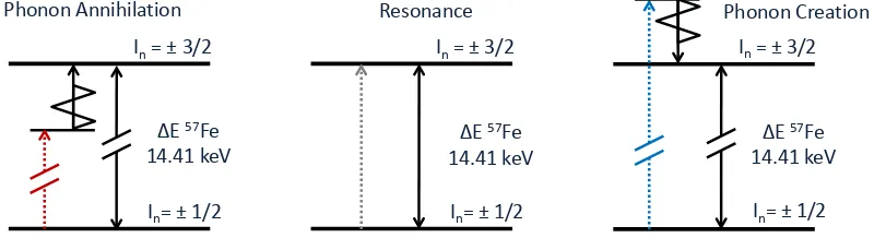
The NRIXS technique probes the phonon spectrum of a material by scanning the energy of the incoming phonon. However, unlike traditional M¨ossbauer spectroscopy which uses the Doppler shift to adjust the incident energies by tens of neV, the high resolution monochromators alter the incoming energy by tens of meV. Detuning the incoming x-ray beam away from the nuclear resonance results in a strong suppression of scattered photons. The incoming x-ray can only excite the narrow nuclear resonance if it obtains additional energy through interactions with the sample. This is done by creating or annihilating a phonon in the sample to obtain the nuclear resonant energy, as shown schematically in Fig. 4.4. As the energy of the incoming photons is varied, only phonons (or

In = 3/2

In= 1/2 ∆E 57_Fe

14.41 keV

In = 3/2

In= 1/2 ∆E 57_Fe

14.41 keV In = 3/2

In= 1/2 ∆E 57_Fe

14.41 keV

Phonon Annihilation Resonance Phonon Creation

In = ± 3/2

In= ± 1/2 ∆E 57_Fe

14.41 keV

In = ± 3/2

In= ± 1/2 ∆E 57_Fe

14.41 keV In = ± 3/2

In= ± 1/2 ∆E 57_Fe

14.41 keV

[image:39.612.131.531.460.569.2]

Phonon Annihilation Resonance Phonon Creation

Figure 4.4: An illustration of the NRIXS excitations processes as the incoming x-ray energy is tuned through the resonant energy. A photon with an energy below the resonant energy (red) must absorb a phonon of the appropriate energy to excite the nuclear resonance. A photon with an energy above the resonant energy must give up energy by exciting a phonon before it can excite the nuclear resonance.

(40)

scattering as a function of energy can be directly mapped as shown in Fig 4.5. At low temperatures

30K

130K

298K

510K

647K

740K

870K

981K

1081K

1180K

-

40

-

20

0

20

40

60

Energy

H

meV

L

Figure 4.5: Raw NRIXS scattering spectra that shown vibrational excitations as a function of scatter-ing energy. Spectra are collected on a polycrystalline sample ofα-57_{Fe over a range of temperatures.}

the number of phonons available for annihillation is quite low, so scattering is suppressed when the incoming photon energy is detuned below the nuclear resonance. However, phonons can still be readily excited at low temperatures by the incoming beam so scattering above the nuclear resonant peak still occurs. At higher temperatures the creation and annihilation components of NRIXS scattering spectra start to be comparable in size.

(41)

processes, and n-phonon processes which scale by the approximate probability of those processes at the temperature of observation. Several phonon DOS spectra from NRIXS measurements ofα-57_Fe

are shown in Fig 4.6.

30K

130K

298K

510K

647K

740K

870K

981K

1081K

1180K

0

10

20

30

40

Energy

H

meV

L

Figure 4.6: Phonon DOS of α-57Fe at a range of temperatures.

(42)

Chapter 5

Computational Methods

5.1

Computational Quantum Mechanics

The development of quantum mechanics was arguably the most significant advance in understanding the physical behavior of materials in the 20th century. Quantum mechanics provides a methodology for predicting how atoms and electrons behave in different spatial configurations. But while quantum mechanics is an extremely accurate formalism for describing the behavior of matter in simple systems like the quantum harmonic oscillator, applying quantum mechanics robustly to less idealized many-body systems requires much mathematical rigor and is often intractable [62]. For systems with several atoms, one must consider the full three dimensional wavefunction character of every nucleus, every electron, and the interactions between them. The time-independent Schr¨odinger equation provides a physical description of matter in the ground state through the expression,

ˆ

HΨ =EΨ, (5.1)

whereE is the scalar ground state energy, ˆH, the Hamiltonian operator, and, Ψ, the system wave-function that is an eigenvector of the Hamiltonian. When one considers the interactions of Ni

ionic cores withNeelectrons, the Hamiltonian operator is recast to enumerate the relevant physical

interactions as

ˆ

HΨ ={− ¯h

2

2me Ne X

j=1

∇2₋¯h 2 2 Ni X u=1 ∇2 Mu + Ne X j,k=1 k<j e2

|rj−rk|

+

Ni X

u,v=1 v<u

ZuZv

|ru−rv|

− Ne X j=1 Ni X u=1 eZu

|rj−ru|

}Ψ =EΨ

(43)

systems went unexploited for many decades.

Walter Kohn was awarded the 1998 Nobel prize in chemistry“for his development of the density-functional theory” [8]. Density-functional theory solves the Schrödinger equation in 5.2 by making a few key assumptions and several clever observations to provide computationally-tractable predictions of real material systems [62, 63]. These points are briefly summarized here. The first inherent assumption is the Born-Oppenheimer approximation, which states that the ions can be assumed stationary on the time scale of electronic interactions, which is justified by the large mass mismatch between the two [62]. This eliminates the second term of Eq. 5.2, and provides constant values for the fourth term. The Kohn-Hohenberg theorems state that the ground state energy of the Schrödinger equation is a unique functional of the electron density, and the energy density that minimizes the functional is the true ground state electron density of the Schrödinger equation [63, 64]. The energy of the configuration can be then computed by finding the proper electron density (a 3-dimensional function), rather than the electron wavefunction (a 3Ne dimensional function). Kohn and Sham

approached the problem by assuming a separable set of electron wave functions that satisfy individual electron Hamiltonians, called the Kohn-Sham equations (which are dependent on knowledge of the total electron density), and wrapping the unknown bits of physics into an exchange-correlation potential Vxc which is necessarily approximated [65]. The single electron Hamiltonian can then

be solved self-consistently until the electron density calculated from the solution wave functions is sufficiently similar to the electron density used to compute those wavefunctions.

This is a very brief summary of the merits of DFT, but the creation of this methodology has spawned a number of first principles methods that provided useful predictions of real materials behavior. DFT simply requires information on the ions in a material and their locations, then the ground state energy of this configuration can be calculated. From these electron energy calculations, electronic band structures provide information on electronic transitions. Additionally, the structural arrangements of atoms input into DFT can be refined to find the lowest energy configuration for the symmetry of the system. Multiple structural symmetry arrangements may be calculated to find the relative energy cost of different crystal structures, and thus the energy competition of different material phases can be analyzed at 0K (the ground state).

(44)

of the equilibrium unit cell atomic structure. These adaptations are more computationally costly because they require large supercells and many additional steps, but they are routinely performed as part of computational DFT studies today.

Density functional theory is an extremely powerful tool and has fueled a revolution in materials physics, however it is an inherently ground state methodology, providing properties at 0K. Real ma-terials, however, are very rarely prepared or used under such conditions. More recent developments have focused on adapting this methodology to explain properties of materials at the ground state, and non-equilibrium behavior. For instance if we are interested in phase diagrams of materials (which I am) we need to consider the energy and entropy of materials at finite temperatures. This returns us to dealing with non-harmonic effects like thermal expansion, which plays an important role in material phase stability and entropy at finite temperatures. There is a DFT approach to thermal expansion with a quasi-harmonic model, although typically different from the formalism developed in Chapter 3. Typical DFT quasi-harmonic thermal expansion is calculated by minimizing the free energy of the material (including electronic and vibrational entropic contributions) with respect to the volume of the structure. This is computationally expensive because it requires iteratively cal-culating vibrational frequencies with the methods described above. Nevertheless, it does provide a completely first principles approach to thermal expansion that does not require experimental input on thermal behavior.

(45)

Ab Initio Molecular Dynamics (AIMD) is a combination approach that uses DFT within each MD time step to realize quantum mechanical behavior at finite temperatures and time scales [66]. This hybrid approach is more computationally expensive than either method in isolation, but it provides benefits that could not be realized by either individually. AIMD has been increasingly utilized to examine the finite temperature behavior of materials, including thermal expansion and high temperature phonon behavior. Methods for extracting vibrational information from AIMD are still an active field of study, with very promising early results [71, 72]. They present a unique opportunity to examine computed vibrational material behavior beyond the limitations of the harmonic and quasi-harmonic models without many-body perturbation theory.

5.2

Born von-K´

arm´

an Fitting of Phonon Spectra

The harmonic model for lattice vibrations constructed in Section 2.2 can be readily applied to ex-perimental measurements given the proper set of assumptions, as noted in Section 2.3. Often called the Born von-K´arm´an (BvK) model, this formalism relates interatomic force constants of crystalline solids to phonon frequencies [11]. To solve for phonon frequencies, the number of interatomic inter-actions in the dynamical matrix is typically limited to the first few nearest-neighbor interinter-actions. This truncation of interaction forces limits the size of the dynamical matrix (which might otherwise be as large as the square of the number of atoms involved). Short-range forces are quite physically reasonable for well behaved materials. The dynamical matrix can then be solved for specific phonon frequencies along the direction of interest ink-space, assuming one has the interatomic force con-stants in the dynamical matrix D(k). The interatomic force constant elements of the dynamical matrix are defined as derivatives of the crystal potential, but this potential, even if harmonic, cannot be derived analytically for the response of real solid material.

When experimental phonon dispersion are available, the elements of the dynamical matrix can be fit to observed phonon energies and momenta by a least squares approach, by constructing a linear set of equations for each observed frequency,

M         ω2 1 ω2 2 .. .

ω_N2

               

1(k1) 2(k2)

.. .

N(kN)

        =        

D(k1) D(k2)

.. .

D(kN)

               

1(k1) 2(k2)

.. .

N(kN)

        .

(46)

dispersion fits [12] are

K1NN=



   

1XX 1XY 1XY

1XY 1XX 1XY

1XY 1XY 1XX



   

<

The Phonon Thermodynamics of Iron and Cementite

Phonon thermodynamics of iron and cementite

Abstract

Contents

List of Figures

List of Tables

Iron and Steel - Ancient History

increasing C content (at. %)

The Dawn of Thermodynamics

Chapter 2

Phonons

Observations of Phonons

Thermodynamics

Debye Model

research papers

Quasi-Harmonic Models

ΓTHTL

Rayne

0

Anharmonic Effects

Chapter 4

∆E 57Fe = 14.41 keV

Nuclear Forward Scattering

Nuclear Resonant Inelastic X-ray Scattering

0

Energy

0

Energy

Born von-K´