DOI: 10.1534/genetics.108.100032
Detecting Selective Sweeps: A New Approach Based
on Hidden Markov Models
Simon Boitard,*
,1Christian Schlo
¨tterer
†and Andreas Futschik*
*Institute of Statistics and Decision Support Systems, University of Vienna, 1010 Vienna, Austria and†Institut fu¨r Populationsgenetik, Veterina¨rmedizinische Universita¨t, 1210 Vienna, Austria
Manuscript received December 22, 2008 Accepted for publication January 29, 2009
ABSTRACT
Detecting and localizing selective sweeps on the basis of SNP data has recently received considerable attention. Here we introduce the use of hidden Markov models (HMMs) for the detection of selective sweeps in DNA sequences. Like previously published methods, our HMMs use the site frequency spectrum, and the spatial pattern of diversity along the sequence, to identify selection. In contrast to earlier approaches, our HMMs explicitly model the correlation structure between linked sites. The detection power of our methods, and their accuracy for estimating the selected site location, is similar to that of competing methods for constant size populations. In the case of population bottlenecks, however, our methods frequently showed fewer false positives.
A
DVANCES in genotyping and sequencing technol-ogy have made it feasible to scan a large amount of DNA sequence data for genes that underwent a recent event of positive selection. Since selective sweeps affect the patterns of genetic variation also in some neighbor-hood of the selected locus, such scans are also known as ‘‘hitchhiking mapping’’ (Maynard Smithand Haigh1974). The patterns that are usually searched for in a population genetic sample are a lower number of segre-gating sites (Kaplanet al.1989), a skewed site frequency
spectrum with many low-frequency and high-frequency derived alleles (Braverman et al. 1995; Fay and Wu
2000), and a modified linkage disequilibrium structure (Kimand Nielsen2004; McVean2006; Stephanet al.
2006; Pfaffelhuberet al.2008).
Several statistical methods have been developed to detect signatures of selective sweeps. Most of them rely on the computation of some summary statistics of the data at each locus; see, for instance, Teshimaet al.(2006)
for a review on this strategy. This approach, however, im-plies a loss of information and brings the difficult ques-tion of the best summary statistics to use. An important improvement has been achieved by Kimand Stephan
(2002), who proposed to compute the maximum com-posite likelihood of the observed allele frequencies for a family of models involving a selective sweep and to com-pare it with the composite likelihood of the same data under a model without selective sweep. With this ap-proach, the full site frequency spectrum information is used, while also taking into account the spatial pattern of genetic diversity that is shaped by recombination.
However, this method is sensitive to demographic ef-fects, because the likelihoods are derived under a model that assumes a constant population size. To overcome this problem, Nielsenet al.(2005) proposed to estimate
a background frequency spectrum from the data, rather than computing it under the hypothesis of a constant size population. Jensen et al. (2005) developed a
goodness-of-fit test in the same spirit. Both methods provide an efficient control of the rate of false positives in the case of an expanding population, but still fail to do so in a wide range of bottleneck scenarios ( Jensenet al.
2005; Williamsonet al.2007). As an alternative, Liand
Stephan (2005, 2006) proposed to estimate the
de-mographic history of the population under study and to compute the likelihoods using simulations that took into account this demographic information. To also use information concerning the linkage disequilibrium pattern, Kimand Nielsen(2004) proposed to compute
the composite likelihood using two-locus haplotype data instead of single-locus allele data. They observed, however (see also Jensenet al.2007), that the
improve-ment compared to the original method of Kim and
Stephan(2002) was not significant. To date, no method
achieves both the high power of the original method of Kimand Stephan(2002) and a reasonable robustness
against past bottleneck events.
The above-mentioned composite-likelihood methods make the simplifying assumption that the allele fre-quencies observed at two close sites are independent random variables. These random variables are indirectly correlated, because the distance from the selected site is taken into account when computing their distributions. However, by assuming that the probability distribution of allele frequencies is a deterministic function of the 1Corresponding author: UR444 Laboratoire de Ge´ne´tique Cellulaire,
INRA, Chemin de Borde Rouge, BP 52627, 31326 Castanet Tolosan Ce´dex, France. E-mail: [email protected]
distance to the sweep, composite-likelihood methods do not capture the stochasticity of the genealogies along the sequence and the correlation pattern resulting from this stochasticity. This issue is addressed by our alternative approach based on hidden Markov models (HMMs). Hidden Markov models allow the hidden state, which should be thought of as a representation of the gene-alogy, to evolve stochastically along the sequence. Al-though the genealogy of a sample is not strictly Markovian along the sequence (Wiufand Hein1999),
the approximation seems reasonable, given that most of the information about the genealogy at one site is provided by the genealogy at the previous site (assuming an arbitrary direction on the sequence). This assump-tion was successfully used, for instance, by Husmeier
and Wright(2001) for detecting recombination events
and by Hobolthet al.(2006) for inferring speciation
times and ancestral population sizes between human, chimp, and gorilla. In addition, HMMs in general benefit from very efficient estimation and prediction algorithms and are already widely used in bioinfor-matics for sequence analysis (Durbinet al.1998; Siepel
and Haussler2004).
Here, we introduce HMM methods for the detection of selective sweeps. Using computer simulations, we show that these methods have a high power for detecting selective sweep events in a population of constant size. Compared to methods that have a similar power in the case of a constant size population, we also show that they often have similar or lower rates of false positives due to demographic events such as population expansions or bottlenecks.
METHODS
Suppose we have a sample consisting ofnaligned DNA sequences of lengthLtaken from the same population. Using these data, we wish to determine whether a selec-tive sweep has occurred in the corresponding chromo-somal region. Fori¼1,. . .,L, letYi¼1,. . .,n1 be the number of derived alleles at sitei, assuming an infinite site model. Whether an allele is ancestral or derived can be determined by looking at an outgroup. To take benefit from the lower polymorphism level expected in the vicinity of the selected locus, we also include the nonsegregating sites in the model. In our simulations, we setYito 0 for those sites, corresponding to the output produced by the software we used to simulate sequences [SelSim (Spencerand Coop2004)]. In practice,
distin-guishing between the statesYi¼0 andYi¼nwould be an option that might lead to a slight increase in per-formance and could easily be implemented.
Furthermore, if no reliable outgroup data are avail-able, Yi could easily be defined as the smaller of the counts of the two alleles, thus using the folded frequency spectrum. We do not, however, consider this case in the present study.
In our model,Yi¼0,. . .,n1 is the observed state at sitei. The hidden stateXiindicates whether sitei has been affected by selection. WhileXishould ideally repre-sent the genealogy of the sample at sitei, and thus have an infinite number of possible values, we chose to focus on a simplified model with only three hidden states: ‘‘neutral,’’ ‘‘intermediate,’’ and ‘‘sweep.’’ A site is in a sweep state when it is very close to the selected locus. Its site frequency spectrum is strongly influenced by the sweep. The inter-mediate state applies to those loci that are only slightly influenced by the sweep because of their larger distance to the selected locus. One could obviously consider models with more hidden states, but such models did not lead to a noticeable improvement of our results.
The assumption that X ¼X1,. . ., XL is a first-order Markov chain and that theYi’s are independent condi-tionally onX(the distribution ofYithus depends only onXi) leads to a HMM. Its full description requires us to specify the following components: (i) the transition matrix between hidden states, (ii) the probability distribution of the initial hidden stateX1, and (iii) the emission probabilities,i.e., the probability distribution ofYigiven a hidden stateXi.
We put the following constraints on the transition matrix:
i. The probability that the hidden chain moves di-rectly from the neutral state to the sweep state or the reverse is set to zero. This is because we expect a gradual shift in the site frequency spectrum along the sequence and do not want to detect a random and localized loss of diversity.
ii. From the intermediate state, the transition proba-bilities to the neutral state and to the sweep state are the same.
iii. The probability of staying in the same state must be nearly equal among states.
If one state has a higher probability, we indeed observed that the most likely hidden chain was generally staying always in this state. According to these con-straints, we choose a transition matrix of the form
T ¼
1p p 0
p=2 1p p=2
0 p 1p
0 @
1 A;
whereTj,kdenotes the transition probability from statej to statek. The indexj¼1 refers to the neutral state,j¼2 refers to the intermediate state, andj¼3 refers to the sweep state. The larger p is chosen, the more sweeps tend to be detected. We therefore use the parameterpto calibrate the false positive rate of the HMM under the null model of no sweep (see theDetecting selection from a samplesection). For any value ofp, the Markov chainX
has the stationary distribution (p1,p2,p3)¼(0.25, 0.5, 0.25), wherepj¼P(Xi¼j). We assume thatX1is drawn
probability of detecting a sweep will not depend on the position of this sweep within the sequence.
If one has relevant information about the proportion of the analyzed sequence influenced by selection, one might want to modify the transition matrix to obtain a stationary distribution reflecting this information.
We considered different strategies for computing the emission matrix, leading to the following HMMs:
HMMA: The emission probabilities in all hidden states are computed according to the formulas by Kimand
Stephan(2002).
HMMB: The emission probabilities are determined using the approach described by Nielsen et al.
(2005).
HMMB-SEG: The same model as HMMB, except that only segregating sites are considered.
More details about these models can be found below. Two further models are also discussed in the supple-mental material.
KIM and STEPHAN’s (2002) approach (HMMA): The
emission probabilities in this model are taken from Equations 3–5 derived by KIM and STEPHAN (2002). These formulas approximate the probability of observ-ingkderived alleles (k¼1,. . .,n1) in a sample of size
n, both for neutral sites and for sites linked to a selected site. They assume that the sweep has just occurred and that the population size has been constant over time. The probabilities depend on the scaled mutation rate
u¼4Nm, whereNis the effective population size andm
the mutation rate per site and generation. In the case of a site linked to a selected site, the expression also depends on the quantityC¼1(1/a)R/s, wheresis the selection intensity at the selected site, a ¼2Ns is the scaled selection intensity, and R is the recombination rate between the selected site and the neutral site.
To determine the emission probabilities in our HMM, we therefore have to choose the value ofu and, in the sweep and intermediate states, the value ofC. Consistent with previous results (WATTERSON 1975), we used Wat-terson’s estimator ofu. Since the selection intensity and the per site recombination rate are rarely known in practice, the choice ofCis more difficult. Furthermore the value ofRappearing in the formula forCdepends on the distance from the selected site that is modeled by our three hidden states. This leads to the rough guideline that the parameter C should be chosen smaller in the sweep state than in the intermediate state, becauseR is smaller in the sweep state. Without additional information, we propose to choose the parameterC to optimize the prediction ability of our HMM. According to our simulations, choosing C ac-cording to a rather weak selection pattern (i.e., a rather large value ofC) under the sweep state tends to improve the sensitivity of the HMM. If the emission patterns in the three hidden states are too similar, on the other hand, the ability of the method to discriminate between
neutral and sweep samples turns out to be low. We therefore choseCby optimizing the detection power in the case of a selective sweep with weak selection intensity (a¼100); for more details see thePower analysissection. We obtainedC¼0.101 for the sweep state andC¼0.411 for the intermediate state. Given that a ¼100, these values correspond toR/s¼0.02 (sweep) andR/s¼0.1 (intermediate). According to our results, this choice leads to a good overall detection power (seeRESULTS).
NIELSEN et al.’s (2005) approach (HMMB):As in KIM
and STEPHAN (2002), NIELSEN et al. (2005) obtain an approximate formula for the probabilityqk* of observing kderived alleles in a sample of sizen(k¼1,. . .,n1) after a selective sweep. However, in contrast to KIMand STEPHAN (2002), each probability qk* is expressed as a function ofq¼(q1,. . .,qn1), whereqkis the probability of observingkderived alleles in a sample of sizenjust before the sweep. In practice, the background probabil-ity distribution q can be estimated by the frequency spectrum in the observed sample. Since we do not know which sites are close to a selected site, the frequency spectrum is estimated from the whole sequence. There-fore the approach will be conservative, if a substantial part of the sequences is affected by selection. The probability distributionq* after the sweep also depends on the additional parameterathat quantifies the relative influence of both the recombination with the selected locus and the selection intensity. Low values of a
correspond to severe hitchhiking effects.
Adapting this approach to our setting, the emission probabilities for the neutral state of our HMM can be taken from the frequency spectrum of the observed sample and the emission probabilities in the interme-diate and sweep states can be computed from Equation 6 in NIELSEN et al. (2005). As with the parameter C
discussed above, the values ofaare chosen to optimize the predictive ability of the HMM. This led toa ¼0.7 for the intermediate state and a ¼ 0.2 for the sweep state.
Segregating sites (HMMB-SEG):SweepFinder (NIELSEN
first compute a sequence of frequencies of the derived allele. We then run the Viterbi algorithm (implemented in the statistical toolbox of MATLAB), to predict the sequence of hidden states X ¼ X1,. . ., XL from the sequence of observed statesY¼Y1,. . .,YL. If at least one site in the sequence has the predicted sweep state, we conclude that a sweep has occurred in the history of the sample. The presence of sites with the predicted in-termediate state does not provide sufficient evidence for a sweep.
The type I error of our method can be defined as the probability of detecting a sweep when analyzing a neutral sample. We control this type I error at level 5% by selecting an appropriate coefficientpin the transition matrix. For a given test sample,pis chosen as follows: (i) Assuming a neutral evolution scenario and a population of constant size, we use ms (HUDSON2002) to simulate a set of samples of the same sizenand the same lengthL
as the test sample; (ii) for an initial valuep0, we analyze these neutral samples as described above and estimate the type I error of the method by the percentage of the samples for which a sweep was detected; and (iii) if this initial error rate is greater (resp. lower) than 5%, we iteratively decrease (resp. increase)puntil the error rate becomes lower (resp. greater) than 5%. We also stop the algorithm ifp becomes.0.1 (even if the error is still
,5%), because we do not want the Markov chain to move too fast from one state to another, which would not be consistent with our idea of modeling the correlation between close sites. Forp¼0.1, the expected number of sites the chain stays in the same hidden state is equal to 10. The quantitydpthat is added or subtracted topat each iteration is small compared top0. The value ofp returned by this procedure is then used for the analysis of the test sample.
Note that the simulation of samples under neutrality described at step i requires the specification ofuandr. In practice, some estimates of these parameters may be found in the literature for the population where the test sample is from. If this is not the case, we suggest estimatinguandrdirectly from the test sample.
One alternative prediction approach, based on the estimation of the posterior probabilities of the sweep state at each sequence position, is briefly covered in the supplemental material.
Power analysis:We performed computer simulations to assess the ability of the various HMM methods to detect a selective sweep (Tables 1–3). We considered different values of the scaled selection intensityaand the timetsince the fixation of the positively selected allele. The per site scaled mutation rateuand the per site scaled recombination rater¼4Nrwere chosen as 0.005 and 0.02, respectively. While most of the classical tests for detecting natural selection require data from independent loci, the proposed HMM methods can be used for analyzing DNA sequences of any length. It seems thus natural to take advantage of this feature to
analyze rather long sequences. Here we considered sequences of length 100 kb and a constant sample size
n¼30. The influence of Landnon the power of the HMMs is covered in supplemental Table S3.
For a given set of parameter values, we simulated 400 samples under selection using SelSim (SPENCER and COOP2004).
To calibrate the transition matrix, neutral samples were simulated with the trueuandr. Since these true parameters will be usually unknown in practice, we also tried to estimate them independently for each test sample. We tried this approach for one set of parameter values and estimatedr using PHASE (version 2.1) (LI and STEPHENS2003; CRAWFORDet al.2004) andu, using Watterson’s estimator. This led to very similar results as in the case of known parameter values (not shown). This might have been expected, because these estimators are generally accurate when applied to populations with constant size. Assuming known values for u and r
considerably reduces the computation time, because the same 200 neutral samples (and thus the samep) can then be used for the 400 test samples.
We estimated the power of a method by the percent-age of test samples for which a sweep was detected. To also investigate the accuracy of the estimated sweep position, we introduce the notion of a ‘‘sweep window,’’ by which we mean a set of consecutive sites with the pre-dicted hidden sweep state. When analyzing a sample, we recorded the number of these windows as well as their length and position. Because of the Markov structure of the hidden state sequence and the fact that the prob-ability of moving from one hidden state to another is very low (otherwise the type I error of the methods would always be very high), we generally observe only few sweep windows in one sequence. For a sample that is simulated under selection, we ideally want to get only one sweep window of relatively small length and in-cluding the selected site (see Figure 1). Our simulation results (see the next section) actually show that this was in most cases the pattern that we observed.
Scenarios with variable population size: The expan-sion and bottleneck scenarios studied in Tables 4 and 5 were simulated using ms, with the same values ofn,L,u, and r as in the power analysis. We simulated 100 test samples for each scenario and analyzed them with HMMA and HMMB. To account for the fact that the estimators ofranduare usually biased for populations with varying size, we did not use the true values of these parameters for adjusting the transition matrix of the HMMs. For each test sample, we instead estimatedrand
ufrom the data and simulated 100 independent neutral samples on the basis of these values.
HMMA is related to CLsw, because its emission matrix is computed from KIM and STEPHAN’S (2002) formulas. Similarly, the emission matrices in HMMB and HMMB-SEG, and the composite likelihood in SweepFinder, are computed from the empirical frequency spectrum combined with NIELSENet al.’s (2005) formulas.
The statistical model behind SweepFinder and CLsw is, however, quite different from the one used for our HMMs. These methods scan a large number of positions in the sequence and look for the one that is the most likely to be a selected site. (For the analysis with Sweep-Finder, we took a step of 40 bases between two positions. For CLsw, the moves between positions are stochastic
and handled by an optimization algorithm, starting from a set of 16 locations equally spaced along the sequence.) At each position, a composite-likelihood value, measuring the evidence for a sweep, is computed. Unlike our proposed hidden Markov models, the method takes into account the exact distance from the hypothetical selected site when computing the contri-bution of a site to the likelihood. On the other hand, the correlation between close sites is taken into account more realistically in a hidden Markov context. One other important point is that HMMA, HMMB, and CLsw use the information from all the sites, while HMMB-SEG and SweepFinder consider only the segregating sites. TABLE 1
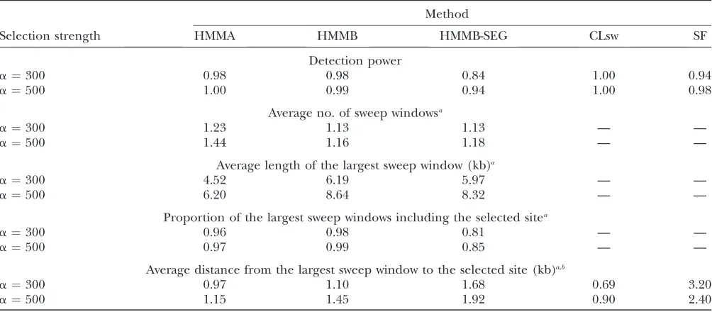
Prediction ability of the HMM methods and of composite-likelihood methods
Method
Selection strength HMMA HMMB HMMB-SEG CLsw SF
Detection power
a¼300 0.98 0.98 0.84 1.00 0.94
a¼500 1.00 0.99 0.94 1.00 0.98
Average no. of sweep windowsa
a¼300 1.23 1.13 1.13 — —
a¼500 1.44 1.16 1.18 — —
Average length of the largest sweep window (kb)a
a¼300 4.52 6.19 5.97 — —
a¼500 6.20 8.64 8.32 — —
Proportion of the largest sweep windows including the selected sitea
a¼300 0.96 0.98 0.81 — —
a¼500 0.97 0.99 0.85 — —
Average distance from the largest sweep window to the selected site (kb)a,b
a¼300 0.97 1.10 1.68 0.69 3.20
a¼500 1.15 1.45 1.92 0.90 2.40
Power to detect a simulated recent selective sweep event (t¼0.001) is shown. HMMA, three-state model; HMMB, three-state model with estimated background emission probabilities; HMMB-SEG, the same as HMMB but with segregating sites only; CLsw, Kimand Stephan’s (2002) method; SF, SweepFinder (Nielsenet al.2005).n¼30,L¼100 kb. Type I error (percentage of falsely detected sweeps using neutral samples) is 5%. —, irrelevant.
a
Among those replicates where at least one sweep is detected.
b
Computed from the center of the sweep window.
TABLE 2
Prediction patterns with multiple sweep windows
No. of sweep windows
1 2 $3
Proportion 0.79 0.19 0.02
Average length of the largest sweep window (kb) 4.60 4.16 4.53
Average length of the second largest sweep window (kb) — 1.54 2.35
Average length of the third largest sweep window (kb) — — 1.31
Largest distance from a sweep window to the selected site (kb)a 0.92 6.78 16.47
Distance from the largest sweep window to the selected site (kb)a 0.92 1.11 1.62
Proportion of the largest sweep windows that include the selected site 0.97 0.92 0.89
Detailed results obtained with HMMA (three-state model) for the sweep scenario of Table 1 witha¼300 are shown. Averages over the replicates where at least one sweep window was detected are displayed.
With Clsw and SweepFinder, a selective sweep is de-tected when the maximum composite-likelihood value exceeds a given threshold. As for the parameterpin our HMMs, this threshold is adjusted to control the type I error of the method. In our simulation study, the same neutral samples were used to adjust the likelihood thres-holds of Clsw and SweepFinder, and the parametersp
of the HMMs.
RESULTS
We present the most significant results of our simu-lation study. We first compare the efficiency of the dif-ferent HMMs for detecting the presence of a selective sweep and estimating the position of the selected site. We also investigate the influence of the strength of selec-tion and of the age of the sweep on the results. The last section deals with the problem of robustness against demographic events such as population growth or bottlenecks.
Comparison of the HMM methods and influence of the sweep intensity:The results obtained with our pro-posed HMMs for recent selective sweeps (t¼0.001) of intensitya¼300 or 500 are provided in Table 1.
For these parameters, all our proposed methods were able to detect the sweep event with high power. Among the samples showing evidence for selection, the average
number of sweep windows was close to one, indicating that in most of the cases there was exactly one sweep window along the sequence. In the rare case when multi-ple sweep windows were detected, we mostly observed one ‘‘large’’ sweep window and one or more ‘‘small’’ windows (an example is provided in Table 2). In most cases, the large window was located very close to the sweep and included the selected site. Consequently, we considered only the largest sweep window for the results shown in Tables 1 and 3.
For the scenarios of Table 1, all methods were able to estimate the location of the selected site accurately. The average size of the sweep window was relatively small (between 4.52 and 8.64 kb depending on the scenario and the method). For HMMA and HMMB, the sweep window included the selected site in at least 96% of the replicates. Any sweep window returned by HMMA or HMMB can consequently be viewed as a confidence interval of level almost 1 for the position of the selected site. Interestingly, the position of the selected site could be well estimated by the center of the sweep window.
Witha¼300, the sweep signal is weaker than witha¼ 500. The detection power was consequently slightly TABLE 3
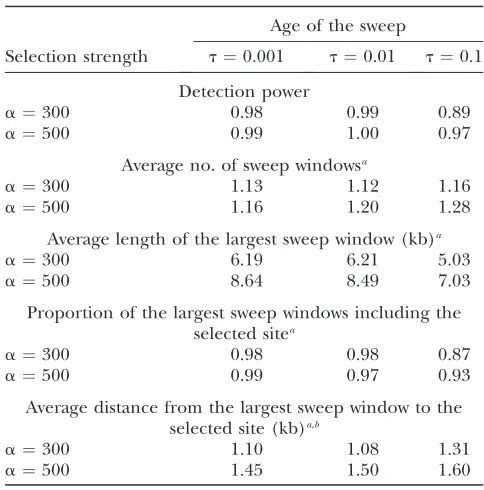
Influence of the age of the sweep
Age of the sweep
Selection strength t¼0.001 t¼0.01 t¼0.1
Detection power
a¼300 0.98 0.99 0.89
a¼500 0.99 1.00 0.97
Average no. of sweep windowsa
a¼300 1.13 1.12 1.16
a¼500 1.16 1.20 1.28
Average length of the largest sweep window (kb)a a¼300 6.19 6.21 5.03
a¼500 8.64 8.49 7.03
Proportion of the largest sweep windows including the selected sitea
a¼300 0.98 0.98 0.87
a¼500 0.99 0.97 0.93
Average distance from the largest sweep window to the selected site (kb)a,b
a¼300 1.10 1.08 1.31
a¼500 1.45 1.50 1.60
Performances of HMMB (three-state model with estimated background emission probabilities) for several values oftand
aare shown.n¼30,L¼100 kb. Type I error is 5%.
aAmong those replicates where at least one sweep is
detected.
b
Computed from the center of the sweep window.
Figure1.—Predicted hidden states along the sequence ob-tained from a typical HMM run for a sample of length 100 kb. ‘‘Neutral’’ states have value 1, ‘‘intermediate’’ states have value 2, and ‘‘sweep’’ states have value 3. The true selected site is indicated by the vertical line.
TABLE 4
False positives in the case of a population expansion
HMMA HMMB CLsw SF
Error rate 0.00 0.01 0.02 0.00
lower for all methods. On the other hand, the location of the sweep was more accurately estimated for smallera. In particular, (i) the average number of sweep windows was closer to one; (ii) the largest sweep window was smal-ler, while it still included the selected site with a very high probability; and (iii) the distance between the center of the largest sweep window and the true position of the selected site was reduced. In our simulation study, we always used the same value of C with HMMA and the same value ofawith HMMB, whatever the value ofain the test samples (which seems reasonable since the true value ofais generally unknown in practice). These choices imply that in all our HMMs the emission pattern in the sweep state is expected in the vicinity of the selected site for a sweep with weak selection intensity. This emission pattern is even more likely to be found in samples ge-nerated under a sweep with strong selection intensity, but it is generally found farther from the selected site. This explains the higher power and the lower accuracy in locating the selected site observed for largera. Taking smaller values ofCwith HMMA andawith HMMB would provide a higher accuracy in estimating the position of the selected site for test samples generated witha¼500. But it would also lead to lower power, especially for the simulations witha¼300 (data not shown).
The performance of the different HMMs is shown in Table 1. First, it appears that HMMB-SEG is not as efficient as the other methods. This is consistent with previous results by KIMand STEPHAN(2002) and KIMand NIELSEN (2004), who reported that the density of segregating sites along the sequence provided useful information. Second, HMMB is slightly more reliable than HMMA. It returned on average fewer sweep win-dows, which more often included the selected site. On the other hand, these windows were a bit larger than with HMMA, and their center was also farther from the sweep. Comparison to other methods:The results obtained with the composite-likelihood methods of KIM and
STEPHAN (2002), implemented in the software CLsw, and of NIELSEN et al. (2005), implemented in the software SweepFinder, are also presented in Table 1. Among all methods, CLsw was the most powerful and the one providing the most accurate estimations of the selected site location. It performed slightly better than HMMA. Among the methods that use an estimated background frequency spectrum, HMMB had a higher power than SweepFinder and the position of the selected site was more accurately estimated by HMMB. The estimate of the selected site position provided by SweepFinder was .20 kb away from the true position in 3.95% of the samples for which a sweep was detected, while this never happened with HMMB. The likeli-hood curve obtained for one such sample is provided in Figure 2. While still estimating the sweep position more accurately, HMMB-SEG was a bit less powerful than SweepFinder. This suggests that the better power obtained with HMMB compared to Sweep-Finder comes from the additional information used by HMMB.
Influence of the age of the sweep:In all our HMMs, the computation of the emission probabilities in the sweep state is based on the assumption of a very recent sweep. The ability to detect older sweeps was tested using simulation scenarios witht¼0.01 andt¼0.1. We report the results of these simulations in Table 3, focusing on HMMB. With t¼0.01, the quality of the predictions was almost the same as witht¼0.001. With
t¼0.1, the results obtained witha¼300 were affected. Both the detection power and the accuracy of localiza-tion decreased. Interestingly, the results obtained with
a ¼500 remained very good even with t ¼ 0.1. Fur-thermore, the difference between HMMB and HMMB-SEG was larger with t¼0.1 than witht¼0.001 (not shown). Using the density of segregating sites seems important to detect older sweeps, for which there is only a small excess of high-frequency derived alleles. TABLE 5
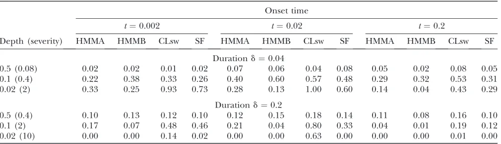
False positive rates under bottlenecks
Onset time
t¼0.002 t¼0.02 t¼0.2
Depth (severity) HMMA HMMB CLsw SF HMMA HMMB CLsw SF HMMA HMMB CLsw SF
Durationd¼0.04
0.5 (0.08) 0.02 0.02 0.01 0.02 0.07 0.06 0.04 0.08 0.05 0.02 0.08 0.05
0.1 (0.4) 0.22 0.38 0.33 0.26 0.40 0.60 0.57 0.48 0.29 0.32 0.53 0.31
0.02 (2) 0.33 0.25 0.93 0.73 0.28 0.13 1.00 0.60 0.14 0.04 0.43 0.29
Durationd¼0.2
0.5 (0.4) 0.10 0.13 0.12 0.10 0.12 0.15 0.18 0.14 0.11 0.08 0.16 0.10
0.1 (2) 0.17 0.07 0.48 0.46 0.21 0.04 0.80 0.33 0.04 0.01 0.19 0.12
0.02 (10) 0.00 0.00 0.14 0.02 0.00 0.00 0.63 0.00 0.00 0.00 0.01 0.00
Impact of population demography: As outlined in several studies (e.g., JENSENet al.2005; TESHIMAet al.2006; THORNTON and JENSEN 2007; WIEHE et al. 2007), de-mographic events such as population expansions or bottlenecks are often falsely detected as selective sweep events, because their effects on the frequency spectrum can be very similar. To investigate the influence of such demographic events, we first studied a neutral scenario where the population size was increased by a factor 10 at timet¼0.25. For each test sample, we estimatedrandu
from the data and simulated independent neutral samples on the basis of these values to adjust the type I errors of the different methods. As expected,rand u
were underestimated. The average ˆr was 0.015 (r ¼ 0.02) and the average ˆuwas 0.002 (u¼0.005).
The rates of falsely detected sweeps obtained with the different methods for this expansion scenario are given in Table 4. The good performance of HMMA and CLsw may seem surprising, given that the frequency spectrum of an expanding population shares two common prop-erties with the one of a selection event: the low number of segregating sites and the high number of low-frequency derived alleles. Two reasons actually explain that no sweep was detected by HMMA and CLsw for the samples of Table 4. First, the emission probabilities in HMMA, and the likelihoods in CLsw, are computed using the estimatedu, which is based on the observed number of segregating sites, and therefore the low level of polymorphism in the data is not detected as an evidence for selection. Second, a relatively high pro-portion of high-frequency derived alleles is expected close to a selected site, but is not found for an expanding population. Confirming the results of NIELSEN et al.
(2005), SweepFinder did not detect selection in the samples of Table 4. This is due to the homogeneity of the frequency spectrum of an expanding population along the sequence. For the same reason, HMMB also per-formed very well.
In the samples simulated under population expan-sion,uwas generally more strongly underestimated than
r. Consequently, in the neutral samples used for adjust-ing the transition matrix of the HMMs, the numbers of derived alleles at two consecutive segregating sites were weakly correlated, which reduces the probability of observing several consecutive segregating sites that all exhibit a sweep pattern. A false detection rate of 5% among these samples would require us to set a rather high transition probabilitypbetween hidden states. But using high transition probabilities between hidden states could lead us to detect very short sweep windows. To make the method more robust against random fluctuations of the frequency spectrum along the se-quence, an upper bound onpturned out to be helpful. In our simulations, the boundp # 0.1 provided satis-factory results.
We also studied the impact of a bottleneck on the predictions and considered several bottleneck scenar-ios. The scenarios were chosen by varying (i) the depthd
of the bottleneck,i.e., the factor by which the popula-tion size is reduced (we assume the populapopula-tion size to be the same before and after the bottleneck); (ii) the durationdof the bottleneck,i.e., the time during which the population size is reduced; and (iii) the onset timet,
i.e., the time since the bottleneck ended. The range of values we chose for these parameters is consistent with those used in recent studies onDrosophila melanogaster
(HADDRILLet al.2005; THORNTONand ANDOLFATTO2006; WIEHE et al. 2007) or on non-sub-Saharan human populations (TESHIMA et al. 2006). As for the samples simulated under population expansion, r and u were estimated from the data for each bottleneck sample.
The percentage of replicates where a sweep was (wrongly) detected is presented in Table 5. In addition to the bottleneck parametersd,d, andt, we indicate for each scenario the severityg¼d/dof the bottleneck as defined in WIEHEet al.(2007). The results obtained with the HMMs and the composite-likelihood methods are qualitatively similar to the ones in (WIEHEet al.2007): The error rates were in general low both for very small (g¼0.08) and very large (g¼10) severities, but they
Figure 2.—Likelihood curves obtained by Sweep-Finder (solid lines) and predicted hidden sequen-ces obtained by HMMB (dashed lines) and HMMB-SEG (dashed-dotted lines) for two samples of sizen¼
were higher for intermediate severities (0.4 or 2). Among the bottlenecks with intermediate severity, the ones with
t¼0.2 caused fewer errors than the ones witht¼0.02 and in most cases fewer errors than the ones witht¼ 0.002 (but see line 2). It is natural to observe lower detection rates in the case of old and less severe bottle-necks, because they have only a small effect on the frequency spectrum. On the other hand, severe bottle-necks do produce a very strong effect on the frequency spectrum, but their effect is quite similar along the sequence, as in a population expansion scenario. The results obtained in such cases can thus be linked to the ones presented in Table 4. Recent bottlenecks with intermediate severity are the most difficult to distinguish from sweeps because they cause a very large variance in the frequency spectrum along the sequence ( JENSEN
et al.2005), with some segments where this spectrum may appear as that of a selective sweep when compared to the global spectrum. Consistent with our results, WILLIAMSON et al. (2007) also found that SweepFinder was conservative for bottlenecks with depth 0.01, anti-conservative for bottlenecks with depth 0.1, and almost unaffected for bottlenecks with depth 0.5.
Besides this overall pattern, large differences were often observed between the different methods. In all the bottleneck scenarios considered here, HMMA had similar or lower false positive rates than CLsw. The dif-ference between the two methods was particularly large for bottleneck scenarios with depth,0.5 (rows 2, 3, 5, and 6 in Table 5). Note that CLsw could be made more robust by using the goodness-of-fit test proposed by JENSENet al.(2005). As shown by the authors, the false positive rates obtained with severe bottlenecks could be substantially reduced using this method. But the use of this correction would also result in a lower detection power. In the scenario witha¼300 studied in Table 1, we indeed found that the detection power, equal to 1.00 without the correction, would fall to 0.73 with the cor-rection. HMMB performed equally well or better than SweepFinder, except for two scenarios. The difference between the two methods was sometimes large, for in-stance, for scenarios with severity 2 (Table 5, rows 3 and 5). For the scenarios with severity 0.4 shown in row 2 of Table 5, ˆuwas large compared to ˆr, which implied that the observations between consecutive segregating sites were highly correlated. The value of p used with the HMMs was quite small in this case. The lower false positive rates obtained by HMMA compared to CLsw may thus be related to the fact that the correlation between sites is taken into account more directly in the HMM framework. For the scenarios with severity .2 (lines 3, 5, and 6 in Table 5), the restriction p # 0.1 turned out to be helpful for avoiding very short artificial sweep windows, as in the case of the expanding population scenario.
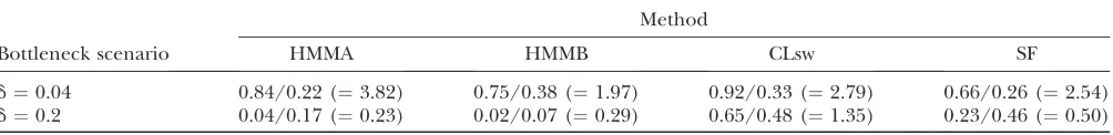
We also looked at sweeps within a bottleneck back-ground and used the software developed by JENSENet al.
(2007) to simulate scenarios where a sweep of intensity
a ¼ 300 occurred during a bottleneck. The power obtained by the different methods is shown in Table 6. We considered two of the bottleneck scenarios in Table 5, both witht¼0.002 andd¼0.1. The first scenario was the one with severity 0.4 and depth 0.1, where both the HMMs and the composite-likelihood methods had high rates of false positives, and where p was small for the HMMs. We can see in Table 6 that all the methods had reasonably high power in this case. The highest ratio between true positives and false positives was obtained with HMMA (4). For the second scenario, the HMMs had almost no power. One way to increase the power in this case would be to relax the constraint p # 0.1. However, we do not recommend this, since the false positive rate when no sweep occurred would then also increase. We note that also CLsw had almost as many false positives as true positives in this case.
In all the scenarios of Table 5 with severity #0.4, HMMA produced fewer false positives than HMMB. This may seem surprising, given that with HMMB the background frequency spectrum is estimated from the data, which is supposed to make the method conserva-tive. We note, however, that this is true only if the effects of demography on the frequency spectrum are similar to the ones of positive selection. This is typically the case for a population expansion, but not for a bottleneck, for which the overall frequency spectrum is actually mod-ified in the ‘‘opposite’’ direction (toward an excess of intermediate-frequency derived alleles) to that for a sweep within a neutral background.
Consequently, the emission probabilities in the sweep state of HMMB correspond to a weaker sweep signal than the ones in the sweep state of HMMA, which explains the higher rate of false positives obtained with HMMB. However, this general idea does not explain the results for the scenarios with severity.2, where HMMB often had fewer false positives than HMMA. Finally, the higher power of HMMA compared to HMMB in the bottleneck scenario with severity 0.4 (Table 6) was not expected, given that for this scenario the rate of false positives was lower with HMMA. While little is known on the combined effects of bottlenecks and sweeps, this re-sult shows that the frequency spectrum observed around a positively selected site can be similar for a population with constant size and for a population that went through a bottleneck of intermediate severity.
DISCUSSION
two different ways of computing the emission probabil-ities of the HMM, using either KIMand STEPHAN’s (2002) or NIELSENet al.’s (2005) approach.
We evaluated the statistical properties of our methods using computer simulations. As illustrated in Tables 1 and 3, both HMMA and HMMB have a very high power for detecting sweeps occurring in a population with constant size. They are powerful even for rather weak selection intensities (a¼300) and quite old sweeps (t¼ 0.1). In most of the replicates, the estimated sweep loca-tion is very accurate. We also found that both HMMA and HMMB are robust against population growth and against bottleneck scenarios with both weak (0.08) and strong (10) severity (Table 5). For bottleneck scenarios with intermediate severity (0.4 and 2), HMMA and HMMB often produced a considerable proportion of false positives, but generally fewer than the composite-likelihood methods of KIM and STEPHAN (2002) and NIELSEN et al. (2005). HMMA performed better than HMMB for bottleneck scenarios with severity#0.4, with both fewer false positives and more true positives (Table 6). Given that both methods performed equally well in Tables 1–4, we would rather recommend using HMMA if we had to choose between both. However, for some bottleneck scenarios with severity 2, HMMB had fewer false positives.
The performance of the HMM approach in compar-ison to composite-likelihood methods depends on the parameters used. In our simulations, SweepFinder was a bit more powerful than HMMB-SEG (Table 1), but with
a¼300 the estimation of the selected site position was less accurate. In some samples where HMMB-SEG could not detect a sweep, SweepFinder did detect it but at a quite wrong position (Figure 2, sample 2). Clsw also performed slightly better than HMMA for detecting selection in a population of constant size. In contrast to HMMA, however, Clsw had a very high rate of false posi-tives under several bottleneck scenarios, up to 1.00 in some cases. For the most difficult bottleneck scenarios, HMMA led to both much fewer false positives and much fewer true positives than CLsw (cf.Table 6, row 2). In other cases, HMMA had a better ratio between true and false positives than Clsw (cf.Table 6, row 1). Overall, it
seems that the significant increase of robustness offered by HMMA is more important than the loss of power, which is small for constant size populations. For com-pleteness, we note that JENSENet al.’s (2005) correction also provided a great gain in robustness in the case of bottleneck scenarios, but led also to a considerable loss of power for constant size populations (only 73% power in the scenario of Table 1 witha¼300).
In addition, the results of Tables 5 and 6 suggest the HMMs perform better in the scenarios where the cor-relation between sites is strong, which is probably due to the fact that the correlation between sites is directly modeled via the Markov structure of the hidden states in a HMM framework. This may thus provide a criterion for deciding when these methods should be preferred over other existing methods. In general, it also seems that the HMM approach is more flexible, because it does not assume that the frequency spectrum is a deterministic function of the distance to the sweep. Hence, it should be less affected by heterogeneities in the recombination rates, for instance, the hot-and-cold spots of recombi-nation, which have been described for humans ( JEFFREYS
et al.2001; GABRIELet al.2002).
The good results obtained by HMMA and HMMB are partly due to the fact that they use all the sites, not only the segregating ones. In our simulations, HMMB per-formed clearly better than HMMB-SEG. Given that we estimate u using Watterson’s estimator, the additional information provided by the nonsegregating sites is not related to the average diversity level, but to its spatial variation along the sequence (KIMand STEPHAN2002). In the composite-likelihood framework, KIM and STE-PHAN (2002) and KIM and NIELSEN(2004) had already observed that using all the sites was a clear advantage. However, NIELSENet al.(2005) pointed out that the usual SNP data sets did not correctly represent the genomic diversity and focused on segregating sites while taking the ascertainment process into account. With the recent advent of high-throughput sequencing, such ascertain-ment problems will disappear in many cases so we think that methods that combine information from the frequency spectrum and from the diversity level provide promising tools for future analysis.
TABLE 6
Detection powervs.false positives for sweeps occurring within a bottleneck
Method
Bottleneck scenario HMMA HMMB CLsw SF
d¼0.04 0.84/0.22 (¼3.82) 0.75/0.38 (¼1.97) 0.92/0.33 (¼2.79) 0.66/0.26 (¼2.54)
d¼0.2 0.04/0.17 (¼0.23) 0.02/0.07 (¼0.29) 0.65/0.48 (¼1.35) 0.23/0.46 (¼0.50)
Even if the HMMs proposed here led to a decrease in the rate of false positives in some bottleneck scenarios, they do not solve the problem completely. Indeed, several bottleneck scenarios with intermediate severities (0.4 and 2) resulted in a high rate of false positives both with the HMM and with the composite-likelihood approach. Such bottleneck scenarios are very difficult to keep apart from selective sweeps, because they induce a high spatial variation in both the diversity level and the site frequency spectrum along the sequence. An alter-native approach for such scenarios would be to use the linkage disequilibrium information. JENSENet al.(2007) studied a bottleneck scenario that was very similar to one where our HMMs had a lot of false positives,i.e., with depth d ¼ 0.1 and durationd ¼0.05 ( Jensen et al.’s Figure 2C), and showed that it could be well distin-guished from a sweep scenario witha ¼500 ( Jensen
et al.’s Figure 2A). They used a statistic introduced by KIM and NIELSEN(2004) and aimed at identifying a linkage disequilibrium structure that is typical for a sweep site.
One alternative way of controlling the errors resulting from demography would be of course to use samples simulated under the ‘‘true’’ demographic scenario for choosing the appropriate value of p in the transition matrix. This would be possible, if the true demographic scenario were known from previous studies, or if it can be inferred by other methods. However, we note that it will be difficult to predict, whether the errors made when estimating the true demographic scenario result in a too conservative or a too liberal test. Indeed, the results of Table 5 suggest that different bottleneck parameters can lead to very different detection patterns.
In our models, the sweep state is characterized by both a low diversity level and an excess of high-frequency deri-ved alleles. This pattern is actually expected in two re-gions flanking the selected site, but not very close to the selected site (FAYand WU2000). One may thus wonder if, in our HMMs, an alternative sweep signal would be a pair of two close sweep windows, rather than one single sweep window. However, the results of Tables 1 and 3 do not support this idea, since in most of the samples only one sweep window was detected.
This could in principle be changed by increasingp, but we observed that the average number of sweep win-dows increases only slowly withp(data not shown). Con-sistent with these results, we also observed that a three-state HMM, where the sweep three-state had essentially no diversity (as in the central region of a sweep), and where the intermediate state had an excess of high-frequency derived alleles [as in the flanking regions (FAYand WU 2000)], did not perform as well as our current models. One reason might be that, for weak selection, the cen-tral region of the sweep is too small. Combining the information from the frequency spectrum and the diversity level seems to be a strength of our HMMs, which makes them powerful even for noisy signals, such as those produced by older sweeps (Table 3).
As for most sweep detection methods (but see HUDSONet al.1987; SCHLO¨ TTERER 2002), we have made the implicit assumption of a homogeneous mutation rate along the entire genomic region surveyed. Hence, a sequence block with lower mutation rate, or a block subject to strong purifying selection, could eventually lead to a signature of a selective sweep. Future studies will be required to determine if the observed heteroge-neity in mutation rates poses a significant problem for our HMM methods.
The HMMs that we presented here have only three hidden states (neutral, intermediate, and sweep) and thus do not fully capture the continuity of the frequency spectrum and of the diversity level along the sequence. We point out that we do not consider these models as a good representation of the reality, but only as good prediction tools. It is well known in statistics that the most sophisticated models are usually not the most effi-cient for prediction purposes. For sweep detection, we actually observed that a HMM with only two states, neu-tral and sweep, performed almost as well as a HMM with three states (supplemental material). We consequently do not think that increasing the number of hidden states would significantly improve our results.
Many of the sweeps that have already been detected in natural populations have stronger selection intensities than those we used in the simulations we presented. Intensities up to a few thousand have been reported, for instance, inD. melanogaster(LIand STEPHAN2006). Since all methods are equally able to detect very strong sweeps, our focus has been on weak sweeps, which are more challenging. In addition, the results in Table 1 indicate that our HMM methods can also easily identify stronger sweeps, because the power increases witha. Due to the larger genomic region affected by a strong selective sweep, however, the precise identification of the target of selection is more difficult for stronger than for weaker selection. This could actually be solved by a second run of the HMM method, using a more skewed emission pattern in the sweep and intermediate states. Alterna-tively, prior information concerning the population or organism of interest could also be used when selecting the model parameters.
In this report, we focused on the most widely studied case of a hard sweep, in which one beneficial mutation arises and subsequently sweeps through the popula-tion until it reaches fixapopula-tion. Recently, it has been suggested that soft sweeps, which involve either re-current mutations or selection from standing varia-tion, are another scenario that should be considered (PRZEWORSKIet al.2005; PENNINGSand HERMISSON2006). We anticipate that the HMM methods introduced here could be modified to account for different selection regimes.
We thank C. Vogl for general discussions and helpful comments on the manuscript. M. H. Quang provided some data-processing routines. K. Thornton kindly helped us with the simulations combining selection and bottleneck. Finally, we are grateful to two anonymous reviewers for useful and insightful comments on the manuscript. This work was financially supported by grants from the Wiener Wissen-schafts-, Forschungs- und Technologiefonds and the Fonds zur Fo¨rderung der Wissenschaftlichen Forschung (P19467-B11).
LITERATURE CITED
BRAVERMAN, J., R. HUDSON, N. KAPLAN, C. LANGLEYand W. STEPHAN, 1995 The hitchhiking effect on the site frequency spectrum on DNA polymorphisms. Genetics140:783–796.
CRAWFORD, D., T. BHANGALE, N. LI, G. HELLENTHAL, M. RIEDERet al., 2004 Evidence for substantial fine-scale variation in recombina-tion rates across the human genome. Nat. Genet.36:700–706. DURBIN, R., S. EDDY, A. KROGHand G. MITCHISON, 1998 Biological
Se-quence Analysis.Cambridge University Press, Cambridge, UK. FAY, J., and C.-I. WU, 2000 Hitchhiking under positive Darwinian
selection. Genetics155:1405–1413.
GABRIEL, S., S. SCHAFFNER, H. NGUYEN, J. MOORE, J. ROYet al., 2002 The structure of haplotype blocks in the human genome. Science
296:2225–2229.
HADDRILL, P., K. THORNTON, B. CHARLESWORTH and P. ANDOLFATTO, 2005 Multilocus patterns of nucleotide variability and the de-mographic and selection history of Drosophilia melanogaster populations. Genome Res.15:790–799.
HOBOLTH, A., O. CHRISTENSEN, T. MAILUND and M. SCHIERUP, 2006 Genomic relationships and speciation times of human, chimpanzee, and gorilla inferred from a coalescent hidden Mar-kov model. PLoS Genet.3(2): e7.
HUDSON, R., 2002 Generating samples under a Wright-Fisher neutral model of genetic variation. Bioinformatics18:337–338. HUDSON, R., M. KREITMANand M. AGUADE´, 1987 A test of neutral
mo-lecular evolution based on nucleotide data. Genetics116:153–159. HUSMEIER, D., and F. WRIGHT, 2001 Detection of recombination in DNA multiple alignments with hidden Markov models. J. Comp. Biol.8:401–427.
JEFFREYS, A., L. KAUPPIand R. NEUMANN, 2001 Intensely punctate mei-otic recombination in the class ii region of the major histocom-patibility complex. Nat. Genet.29:217–222.
JENSEN, J., Y. KIM, V. BAUERDUMONT, C. AQUADROand C. BUSTAMANTE, 2005 Distinguishing between selective sweeps and demography using DNA polymorphism data. Genetics170:1401–1410. JENSEN, J., K. THORNTON, C. BUSTAMANTEand C. AQUADRO, 2007 On
the utility of linkage disequilibrium as a statistic for identifying targets of positive selection in nonequilibrium populations. Ge-netics176:2371–2379.
KAPLAN, N., R. HUDSONand C. LANGLEY, 1989 The hitchhiking effect revisited. Genetics123:887–899.
KIM, Y., and R. NIELSEN, 2004 Linkage disequilibrium as a signature of selective sweeps. Genetics167:1513–1524.
KIM, Y., and W. STEPHAN, 2002 Detecting a local signature of genetic hitchhiking along a recombining chromosome. Genetics 160:
765–777.
LI, H., and W. STEPHAN, 2005 Maximum-likelihood methods for de-tecting recent positive selection and localizing the selected site in the genome. Genetics171:377–384.
LI, H., and W. STEPHAN, 2006 Inferring the demographic history and rate of adaptative substitution in Drosophila. PLoS Genet.2(10): e166.
LI, N., and M. STEPHENS, 2003 Modeling linkage disequilibrium, and identifying recombination hotspots using SNP data. Genetics
165:2213–2233.
MAYNARDSMITH, J., and J. HAIGH, 1974 The hitch-hiking effect of a favourable gene. Genet. Res.23:23–35.
MCVEAN, G., 2006 The structure of linkage disequilibrium around a selective sweep. Genetics175:1395–1406.
NIELSEN, R., L. WILLIAMSON, Y. KIM, M. HUBISZ, A. CLARK et al., 2005 Genomic scans for selective sweeps using SNP data. Ge-nome Res.15:1566–1575.
PENNINGS, P., and J. HERMISSON, 2006 Soft sweeps iii: the signature of positive selection from recurrent mutation. PLoS Genet.2(12): e186.
PFAFFELHUBER, P., A. LEHNERTand W. STEPHAN, 2008 Linkage disequi-librium under genetic hitchhiking in finite populations. Genetics
179:527–537.
PRZEWORSKI, M., G. COOPand J. WALL, 2005 The signature of positive selection on standing genetic variation. Evolution59(11): 2321– 2323.
SCHLO¨ TTERER, C., 2002 A microsatellite-based multilocus screen for the identification of local selective sweeps. Genetics160:753– 763.
SIEPEL, A., and D. HAUSSLER, 2004 Combining phylogenetic and hid-den Markov models in biosequence analysis. J. Comp. Biol.11:
413–428.
SPENCER, C., and G. COOP, 2004 Selsim: a program to simulate pop-ulation genetic data with natural selection and recombination. Bioinformatics20(18): 3673–3675.
STEPHAN, W., Y. SONGand C. LANGLEY, 2006 Hitchhiking effect on linkage disequilibrium between linked neutral loci. Genetics
172:2647–2663.
TESHIMA, K., G. COOPand M. PRZEWORSKI, 2006 How reliable are em-pirical genomic scans for selective sweeps. Genome Res.16:702– 712.
THORNTON, K., and P. ANDOLFATTO, 2006 Approximate Bayesian inference reveals evidence for a recent, severe bottleneck in a Netherlands population of Drosophila melanogaster. Genetics
172:1607–1619.
THORNTON, K., and J. JENSEN, 2007 Controlling the false-positive rate in multilocus genome scans for selection. Genetics175:737–750. WATTERSON, G., 1975 On the number of segregating sites in genetical models without recombination. Theor. Popul. Biol.7:256–276. WIEHE, T., V. NOLTE, D. ZIVKOVIC and C. SCHLO¨ TTERER, 2007 Identification of selective sweeps using a dynamically ad-justed number of linked microsatellites. Genetics175:207–218. WILLIAMSON, S., M. HUBISZ, A. CLARK, B. PAYSEUR, C. BUSTAMANTEet al., 2007 Localizing recent adaptive evolution in the human ge-nome. PLoS Genet.3(6): e90.
WIUF, C., and J. HEIN, 1999 Recombination as a point process along sequences. Theor. Popul. Biol.55:248–259.