ABSTRACT
WU, QIFENG. Predictions of Microstructurally Induced Failure Nucleation and Propagation in High Strength Martensitic Steel Alloys. (Under the direction of Professor Mohammed A. Zikry).
A dislocation-density based crystal plasticity formulation, which accounts for martensitic microstructures, variant morphologies, orientation relationships (ORs), retained austenite, carbide precipitates, dislocation-density evolution, and dislocation-density grain boundary (GB) interactions, has been developed to investigate large inelastic deformation and failure modes, such as quasi-static and dynamic crack nucleation and growth and diffusion assisted hydrogen embrittlement in high strength martensitic steels.
hydrogen diffusion affects dislocation-density evolution and subsequent martensitic
embrittlement. Stresses along the three cleavage planes and the six hydrogen embrittlement fracture planes were monitored to characterize the competition mechanism between cleavage fracture and hydrogen diffusion assisted fracture along preferential crystallographic planes.
Dislocation-density evolution and accumulation ahead of the crack front had a dominant effect on crack propagation, and large dislocation-density generation ahead of crack front blunted crack and inhibited crack propagation, which significantly increased fracture toughness. GBs and blocks with large misorientations resulted in dislocation-density pile-ups, high local stresses, and this resulted in crack nucleation. Hydrogen diffusion was shown to suppress dislocation density emission, which led to martensitic embrittlement and subsequent fracture at low nominal strains.
Retained austenite resulted in lower interfacial stresses and larger plastic
deformations, and also resulted in dislocation-density accumulation around crack fronts for quasi-static and dynamic fracture. This decreased overall strength and increased the
toughness of martensitic steels due to enhanced slip activity along austensite-martensite interfaces. Carbide precipitates resulted in higher local stresses and lower plastic
crack front resulted in large pressure gradient and hydrogen accumulation, and this led to a significant reduction of the critical fracture stress and accelerated crack growth.
These validated predictions indicate that the collective and interrelated effects of the orientation and size of martensitic blocks and packets, variants and GBs, the distribution of retained austenite and carbide precipitates can be fundamentally optimized at the
Predictions of Microstructurally Induced Failure Nucleation and Propagation in High Strength Martensitic Steel Alloys
by Qifeng Wu
A dissertation submitted to the Graduate Faculty of North Carolina State University
in partial fulfillment of the requirements for the degree of
Doctor of Philosophy
Mechanical Engineering
Raleigh, North Carolina 2015
APPROVED BY:
_______________________________ ______________________________ Professor Mohammed A. Zikry Professor Kara Peters
Committee Chair
DEDICATION
BIOGRAPHY
Qifeng Wu was born and raised in Nanchong, Sichuan, China. He attended Huazhong University of Science and Technology, China for his undergraduate studies in Naval
Architecture and Ocean Engineering. He received a bachelor degree in Naval Architecture and Ocean Engineering in June of 2009. After graduation, he attended North Carolina State University (NCSU) for his graduate studies in Mechanical Engineering, and earned a Master of Science degree in Mechanical Engineering in May of 2011. In the summer of 2011, he continued his studies in PhD program in Mechanical Engineering at NCSU under advisor Professor Mohammed A. Zikry. The research related to this dissertation has generated the following research papers:
Q. Wu, P. Shanthraj, and M.A. Zikry, Modeling the heterogeneous effects of retained austenite on the behavior of martensitic high strength steels, International Journal of Fracture, 184, 241-252, 2013.
Q. Wu and M.A. Zikry, Microstructural modeling of crack nucleation and propagation in high strength martensitic steels, International Journal of Solids and Structures, 51, 4345-4356, 2014.
P. Khanikar, Q. Wu, and M.A. Zikry, Dynamic fracture of layered aluminum composites: microstructural modeling, International Journal of Impact Engineering, under review, 2014. Q. Wu and M. A. Zikry, Modeling of diffusion assisted hydrogen embrittlement failure in high strength martensitic steels, submitted, 2014.
ACKNOWLEDGMENTS
I would like to first acknowledge my advisor, Dr. Mohammed Zikry for teaching me how to conduct good research. Without his patience, encouragement and guidance, the dissertation would be impossible. I would also like to thank my doctoral committee
members: Dr. Mohammed Zikry, Dr. Kara Peters, Dr. Yong Zhu and Dr. Donald Brenner for their willingness to be my committee members and providing valuable comments and
suggestions on my research.
I would like to thank my coworkers in the Computational and Experimental
Mechanics of Materials Lab. Dr. Tarek Hatem, Dr. William Lee, Dr. Pratheek Shanthraj, Dr. Siqi Xu, Dr. Prasenjit Khanikar, Dr. Letisha McLaughlin, Dr. Darrell LaBarbera, Shoayb Ziaei, Judith Brown, Bingxiao Zhao, Matt Bond, Tamir Hasan, Michael Rosenberg and Ismail Mohamed. I would specially like to thank Dr. Pratheek Shanthraj for his guidance on Crystal2D.
TABLE OF CONTENTS
LIST OF TABLES ... vii
LIST OF FIGURES ... viii
CHAPTER 1: Introduction ... 1
1.1 Overview ... 1
1.2 General Research Objectives and Approach ... 5
1.3 Dissertation Organization ... 6
CHAPTER 2: Microstructure Modeling and Representation ... 8
2.1 Multiple Slip Crystal Plasticity Formulation ... 8
2.2 Dislocation-Density Evolution ... 10
2.3 Dislocation-Density GB Interaction Scheme ... 15
2.4 Thermo-Mechanical Coupling ... 17
2.5 Stress Assisted Hydrogen Diffusion ... 17
2.6 Martensitic Microstructural Representation ... 18
2.7 Tables and Figures ... 20
CHAPTER 3: Fracture Approach and Numerical Method ... 23
3.1 Microstructure-Based Failure Criterion ... 23
3.2 Failure Criterion for Hydrogen Embrittlement ... 24
3.3 Failure Criterion for Intergranular Fracture ... 25
3.4 Numerical Implementation of Overlapping Element Method ... 25
3.5 Computational Techniques for Crystal Plasticity ... 27
3.6 Tables and Figures ... 29
CHAPTER 4: The Heterogeneous Effects of Retained Austenite on The Behavior of Martensitic High Strength Steels ... 30
4.1 The Model ... 30
4.2 Results and Discussion ... 32
4.2.1 Retained Austenite-Martensite Interaction ... 32
4.2.2 Effects of Parent Austenite Orientation ... 35
4.2.3 Dynamic Behavior ... 37
4.3 Conclusions ... 38
4.4 Tables and Figures ... 40
CHAPTER 5: Microstructural Crack Nucleation and Propagation in High Strength Martensitic Steels ... 51
5.1 The Model ... 51
5.2 Results and Discussion ... 52
5.2.1 Dislocation-Density Evolution Ahead of Crack Front ... 52
5.2.2 Quasi-Static Crack Nucleation ... 54
5.2.3 Dynamic Behavior ... 57
5.3 Conclusions ... 58
5.4 Tables and Figures ... 60
6.1 The Model ... 72
6.2 Results and Discussion ... 73
6.2.1 Microstructural Dynamic Fracture ... 73
6.2.2 Size Effects: Dynamic Fracture with Refined Blocks ... 77
6.3 Conclusions ... 78
6.4 Tables and Figures ... 80
CHAPTER 7: Hydrogen Embrittlement in High Strength Martensitic Steels ... 91
7.1 The Model ... 91
7.2 Results and Discussion ... 93
7.2.1 Hydrogen Diffusion ... 93
7.2.2 Hydrogen Diffusion Assisted Fracture ... 94
7.2.3 Hydrogen Embrittlement with A Pre-existing Crack ... 98
7.3 Conclusions ... 100
7.4 Tables and Figures ... 102
CHAPTER 8: Transgranular and Intergranular Fracture in Bicrystal Martensitic Steels .... 116
8.1 The Model ... 116
8.2 Results and Discussion ... 117
8.2.1 Microstructural Fracture in Bicrystals with Σ3 Boundary ... 117
8.2.2 Microstructural Fracture in Bicrystals with Σ11 Boundary ... 119
8.3 Conclusions ... 120
8.4 Tables and Figures ... 121
CHAPTER 9: Recommendations for Future Research ... 129
LIST OF TABLES
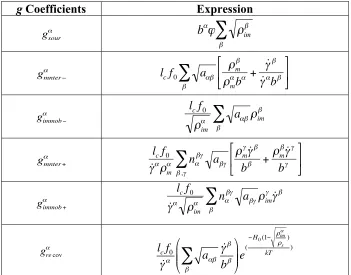
Table 2.1: g coefficients in Eqs. 2.28 and 2.29 ... 20
Table 2.2: The 24 variants corresponding to the K-S OR ... 21
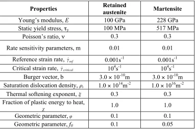
Table 4.1: Material Properties ... 40
Table 5.1: Material Properties ... 60
Table 6.1: Material Properties ... 80
Table 7.1: Material Properties ... 102
LIST OF FIGURES
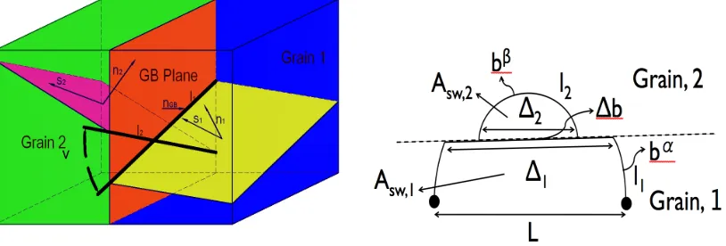
Figure 2.1 Dislocation configuration of a Frank-Read source in the vicinity of a GB. ... 22
Figure 3.1 Decomposition of a cracked element with two overlapping elements. ... 29
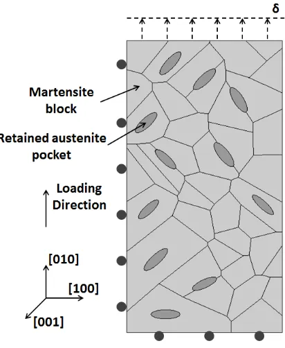
Figure 4.1 Microstructural model and retained austenite pocket, block/packet arrangement 41
Figure 4.2 Nominal stress-strain curve for experimental and numerical model ... 42
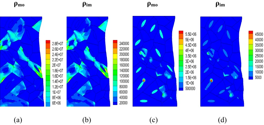
Figure 4.3 Mobile and immobile dislocation densities at a nominal strain of 20% for, (a) and (b) most active slip system in martensite (112)[1 11], (c) and (d) most active slip system in retained austenite (1 11)[011]. ... 43
Figure 4.4 Behavior at a nominal strain of 20%, (a) shear slip, (b) lattice rotation, (c)
normalized total interaction dislocation density, (d) normalized normal stress. ... 44
Figure 4.5 Mobile and immobile dislocation densities at a nominal strain of 20% for the low Euler angle case of (2º, 4º, 8º) for, (a) and (b) most active slip system in martensite
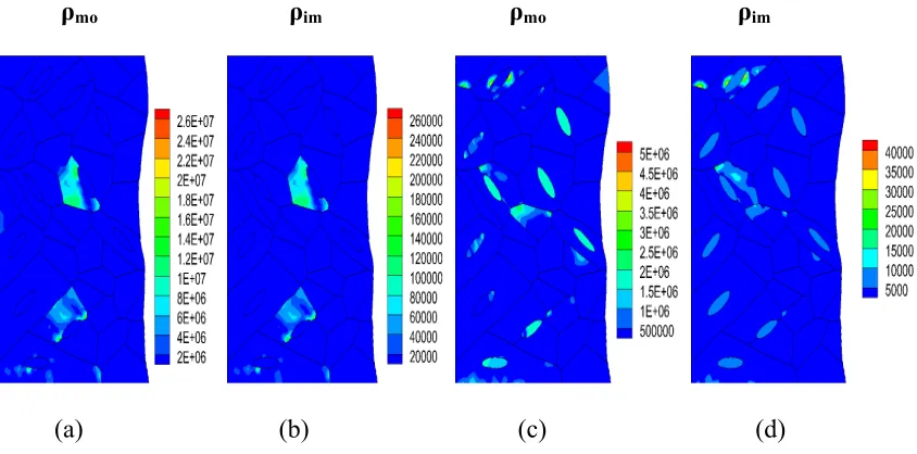
(112)[1 11], (c) and (d) most active slip system in retained austenite (1 11)[011]. ... 45
Figure 4.6 Behavior at a nominal strain of 20% for the low Euler angle case of (2º, 4º, 8º), (a) shear slip, (b) lattice rotation, (c) normalized total interaction dislocation density, (d) normalized normal stress. ... 46
Figure 4.7 Mobile and immobile dislocation densities at a nominal strain of 20% for the high Euler angle case of (15º, 25º, 35º) for, (a) and (b) most active slip system in martensite
(2 11)[11 1], (c) and (d) most active slip system in retained austenite (1 11)[101]. ... 47
Figure 4.8 Behavior at a nominal strain of 20% for the high Euler angle case of (15º, 25º, 35º), (a) shear slip, (b) lattice rotation, (c) normalized total interaction dislocation
density, (d) normalized normal stress. ... 48
Figure 4.9 Nominal stress-strain curves for different parent austenite orientations ... 49
Figure 4.10 Behavior at a nominal strain of 10% for the low Euler angle case of (2º, 4º, 8º) at a strain rate of 5000 s-1, (a) shear slip, (b) lattice rotation, (c) normalized temperature, (d) normalized normal stress. ... 50
Figure 5.1 Microstructural model and distribution of variants in martensitic blocks, (a)
variant distribution for Case I, (b) variant distribution for Case II. ... 61
Figure 5.2 Dislocation generation at, (a) 2% nominal strain, (b) 6.2% nominal strain, (c) 8% nominal strain, (d) 12% nominal strain. ... 62
Figure 5.3 Behavior at 12% nominal strain, (a) shear slip, (b) normal stress ... 63
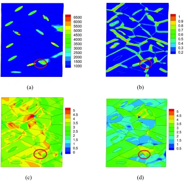
Figure 5.4 Behavior for Case I at 2.6% nominal strain, (a) immobile dislocation density for the active slip system in martensite (121)[111], (b) GB transmission factor for slip system(121)[111], (c) normal stress, (d) maximum stress on cleavage planes {100}. ... 64
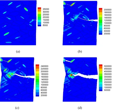
Figure 5.5 Normal stress for Case I at, (a) 6.2% nominal strain, (b) 7.2% nominal strain, (c) 9% nominal strain, (d) 12% nominal strain showing crack nucleation and propagation. ... 65
Figure 5.7 Normal stress for Case II at, (a) 5.8% nominal strain, (b) 9.6% nominal strain, (c) 11.2% nominal strain, (d) 14% nominal strain showing crack nucleation and
propagation. ... 67
Figure 5.8 Stress-strain curves for the two cases. ... 68
Figure 5.9 Normal stress for variant distribution Case II at a strain rate of 5000/s at, (a) 0.6% nominal strain, (b) 4.4% nominal strain, (c) 10% nominal strain, (d) 12.6% nominal strain showing crack nucleation and propagation. ... 69
Figure 5.10 Behavior for variant distribution Case II at a strain rate of 5000/s at 10% nominal strain, (a) shear slip, (b) normalized temperature. ... 70
Figure 5.11 Stress-strain curves for dynamic and quasi-static case. ... 71
Figure 6.1 A schematic diagram of the carbide precipitates, M23C6, in martensitic steels ... 81
Figure 6.2 Microstructural model and distribution of variants in martensitic blocks, (a) case I with 18 blocks, (b) case II with 40 blocks ... 82
Figure 6.3 Behavior at a nominal strain of 1.8%, (a) immobile dislocation density for slip system (211)[111], (b) GB transmission factor for slip system (211)[111], (c) normal stress, (d) shear slip ... 83
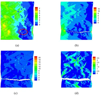
Figure 6.4 (a) maximum stress on cleavage planes {100} at a nominal strain of 1.8%, normal stress at a nominal strain of, (b) 2.6%, (c) 3.8%, (d) 6.6% showing crack nucleation and growth ... 84
Figure 6.5 Behavior at a nominal strain of 3.8%, (a) immobile dislocation density for slip system (110)[11 1], (b) shear slip, GND screw dislocation density for slip system
(12 1)[111] at a nominal strain of, (c) 3.2%, (d) 3.8% ... 85 Figure 6.6 Thermal evolution behavior at a nominal strain of 6.6%, (a) plastic work, (b)
adiabatic temperature, (c) temperature change due to heat conduction, (d) total
temperature ... 86
Figure 6.7 Behavior at a nominal strain of 2.4%, (a) immobile dislocation density for slip system (0 11)[111], (b) GB transmission factor for slip system (0 11)[111], (c) normal stress, (d) shear slip ... 87
Figure 6.8 Normal stress at a nominal strain of, (a) 7.6%, (b) 9.2% showing crack nucleation and growth, (c) shear slip and (d) total temperature at a nominal strain of 9.4% ... 88
Figure 6.9 Comparison of crack length curves ... 89
Figure 6.10 Nominal stress-strain curves at a strain rate of 5000/s ... 90
Figure 7.1 Microstructural model and carbide precipitates M23C6, block/packet arrangement. ... 103
Figure 7.2 Hydrogen diffusion behavior, (a) hydrogen concentration at 2% nominal strain, (b) hydrogen concentration at 6% nominal strain, (c) pressure, (d) norm of pressure gradient. ... 104
Figure 7.4 Diffusion assisted hydrogen cracking behavior, (a) maximum stress on {100} planes at 1% nominal strain, (b) maximum stress on {110} planes at 1% nominal strain, (c) normal stress at 1.8% nominal strain, (d) normal stress at 2.2% nominal strain. .... 106
Figure 7.5 Hydrogen embrittlement behavior at 2.2% nominal strain, (a) pressure, (b) norm of pressure gradient, (c) hydrogen concentration, (d) reduction of critical fracture stress on {110} planes. ... 107
Figure 7.6 Stress-strain curves for the hydrogen embrittlement case, and the case without embrittlement. ... 108
Figure 7.7 Comparison between the hydrogen embrittlement case and the case without embrittlement, total dislocation density generation, (a) for the hydrogen embrittlement case at 2.8% nominal strain, (b) for the case without embrittlement at 10% nominal strain; shear slip, (c) for the hydrogen embrittlement case at 2.8% nominal strain, (d) for the case without embrittlement at 10% nominal strain. ... 109
Figure 7.8 Comparison of GND dislocation density loop between the hydrogen embrittlement case and the case without embrittlement, GND screw dislocation density of slip system
(110)[11 1] for the hydrogen embrittlement case, (a) at 1.7% nominal strain, (b) at 2.8%
nominal strain; GND screw dislocation density of slip system (110)[1 11] for the case
without embrittlement, (c) at 6% nominal strain, (d) at 8.4% nominal strain. ... 110
Figure 7.9 Comparison of crack length for the hydrogen embrittlement case and the case without embrittlement. ... 111
Figure 7.10 Hydrogen embrittlement behavior for the case with a pre-crack at 0.3% nominal strain, (a) pressure, (b) norm of pressure gradient, (c) hydrogen concentration, (d) reduction of critical fracture stress on {110} planes. ... 112
Figure 7.11 Comparison of normal stress at 2% nominal strain with a pre-crack for, (a) the hydrogen embrittlement case and (b) the case without embrittlement. ... 113
Figure 7.12 Comparison of crack length for the hydrogen embrittlement case and the case without embrittlement, with a pre-crack. ... 114
Figure 7.13 Comparison between the hydrogen embrittlement case and the case without embrittlement, (a) the immobile dislocation density for the active slip system
(112)[1 11], for the hydrogen embrittlement case at 2% nominal strain, (b) the immobile dislocation density for the active slip system (112)[111], for the case without
embrittlement at 4% nominal strain, (c) shear slip, for the hydrogen embrittlement case at 2% nominal strain, (d) shear slip, for the case without embrittlement at 4% nominal strain. ... 115
Figure 8.1 CSL grain boundary ... 122
Figure 8.2 Microstructural bicrystal model and distribution of variants in martensitic blocks, (a) case I with Σ3 boundary, (b) case II with Σ11 boundary. ... 123
Figure 8.3 (a) immobile dislocation density and (b) GB transmission factor for slip system (110)[11 1] at a nominal strain of 1%, normal stress at, (c) 6% nominal strain, (d) 6.6% nominal strain showing crack growth. ... 124
Figure 8.5 (a) immobile dislocation density and (b) GB transmission factor for slip system
(110)[1 11] at a nominal strain of 0.8%, normal stress at, (c) 1.2% nominal strain, (d)
1.8% nominal strain showing crack growth. ... 126
Figure 8.6 Behavior at a nominal strain of 1.8%, (a) total dislocation-density generation, (b) shear slip, (c) lattice rotation. ... 127
CHAPTER 1: Introduction
1.1 Overview
Lath martensitic steels, due to their high strength, toughness, and fracture resistance are ideal material choices for critical engineering structures and components. These inherent properties are mainly a result of martensitic steel’s unique lath microstructure, and its
orientation relationships (ORs) with parent austenite grain (Morito et al., 2003; Morito et al., 2006). Furthermore, the strength and toughness of lath martensitic steel are strongly related to block morphology, which is a group of laths with low angle misorientations, and a packet morphology, which is a collection of blocks with the same habit plane (Krauss, 1999; Swarr and Krauss, 1976), and block and packet sizes are proportional to the parent austenite grain size (Morito et al., 2005). Experimental observations have also shown that martensitic packet sizes are related to the size of cleavage facets, due to large misorientations of {100} cleavage planes at packet boundaries, and this affects the fracture toughness of martensitic steel (Wang et al., 2008).
In martensitic steels, ductility and toughness can be improved through retained austenite. Generally, small amounts of retained austenite are frequently observed in
martensitic steel depending on the carbon content and heat treatment conditions (Park et al., 2004; Thomas, 1978). Retained austenite is mainly located at martensitic inter-lath
boundaries and block/packet boundaries (Song et al., 2010; Morito et al., 2011; Ma et al., 2012). These block-like or pockets of retained austenite can improve ductility and toughness, but decrease the strength of martensitic steel (Nakagawa and Miyazaki, 1999; Moor et al., 2008). In addition, the transformation of retained austenite to martensite in the regions close to fracture surfaces has been observed in martensitic steel (Bilmes et al., 2001; Song et al., 2010). These transformations can induce plastic zones, absorb strain energy, and effectively improve fracture toughness.
The strength of steels can be increased through introduction of precipitates (Xu et al., 2011; Ghosh et al., 2005; Zhou et al., 2013), since these fine precipitates can impede
dislocation movement. The strength improvement is related to the size, volume fraction, distribution, and crystal structure of precipitates (Shen and Hansen, 1997; Chen et al., 2014; Lu et al., 2012). Besides improving the strength, the hard precipitates usually reduce ductility and fracture toughness of steels (Chen et al., 2002; Simmons, 1995). Experimental
observations have shown that the hard precipitates can act as the sites of crack nucleation (Yin et al., 2007; Zhang et al., 2001; Du et al., 2012).
precipitate M23C6, where M is mainly Cr and can be replaced with Fe, Mo, Ni (Song et al., 2010; Maruyama et al., 2001). The M23C6 carbide precipitates mainly locate at martensitic block and packet boundaries, and parent austenite grain boundaries (Kipelova et al., 2013; Taneike et al., 2004). The M23C6 carbide precipitates have face centered cubic crystal structure, and have cube-to-cube ORs with parent austenite grain (Shtansky et al., 2000; Kaneko et al., 2011). Since they tend to coarsen easily due to solubility of iron and
chromium, the M23C6 carbide precipitates have a large size of 0.1 – 0.3 µm with a volume fraction of around 2% (Abe, 2008). These large hard M23C6 carbide precipitates at
martensitic block/packet boundaries can act as the sites of crack nucleation (Krauss, 2001), which significantly affect the fracture toughness of martensitic steels.
The fracture toughness of martensitic steels can be significantly affected by environmental factors. Hydrogen embrittlement is a process by which metals and alloys become brittle and fracture due to introduction of hydrogen, which is a result of combined mechanisms that can involve electrochemistry, diffusion, microstructures, fracture
Josephic, 1974), and hydrogen enhanced local plasticity (HELP) (Birnbaum and Sofronis, 1994; Martin et al., 2011).
High strength martensitic steels are extremely susceptible to hydrogen embrittlement, even at very low hydrogen concentrations (Ramamurthy and Atrens, 2013; Nagao et al., 2012; Lee and Gangloff, 2007; Lee et al., 2010). The effects of hydrogen concentration on embrittlement in martensitic steels have been investigated using quasi-static and creep tests, which indicate that hydrogen can decrease tensile strength in a power law manner (Wang et al., 2007; Wang et al., 2005; Kim et al., 2009). Microstructural features, such as grain size, carbide precipitates, and retained austenite, can affect the susceptibility of martensitic steels to hydrogen diffusion and embrittlement (Fuchigami et al., 2006; Kim et al., 1986; Craig and Krauss, 1980). Hydrogen diffusion assisted microstructural fracture in lath martensitic steel occurs on {110} glide planes (Shibata et al., 2012; Kim and Morris, 1983), which is different from the cleavage planes of {100} (Morris, 2011; Guo et al., 2004).
intergranular hydrogen diffusion and embrittlement. However, the critical martensitic characteristics, such as ORs, variant morphologies, parent austenite orientations, initial dislocation densities, retained austenite, carbide precipitates, and crack growth along specific crystallographic planes are not accounted for in these investigations.
All of these investigations indicate that the combined effects of the morphology and crystallography of martensitic blocks and packets, retained austenite, carbide precipitates, and hydrogen diffusion, have a significant influence on the strength, ductility, and fracture toughness, through the dislocation evolution at both the interfaces and the packet and block boundaries, and the complex crack nucleation and propagation.
1.2 General Research Objectives and Approach
The objective of the present work, therefore, is to develop an integrated framework that incorporates microstructural features of martensitic steels, retained austenite and carbide precipitates, such that failure at different scales can be investigated. An essential aspect of the approach is the modeling of crack nucleation and growth along specific crystallographic planes, incompatible interfaces of martensite (b.c.c.) and retained austenite (f.c.c.), and boundaries of martensitic blocks. A fracture method based on the overlap element method of Wu and Zikry (2014) and Hansbo and Hansbo (2004) has been developed to generate failure surfaces as a function of microstructural characteristics, dislocation-density evolution, and martensitic block orientations.
which occur over different scales in crystalline materials. The formulation is based on the framework recently developed by Shanthraj and Zikry (2011) for f.c.c. and b.c.c. crystalline structures. The dislocation-density evolution equations are coupled through the interaction of forest densities, which account for the formation and annihilation of junctions. The evolution equations are coupled to a multiple-slip crystal plasticity formulation, and specialized finite-element techniques (Zikry, 1994) are used to characterize the dominant dislocation-density interaction mechanisms. A dislocation-density GB interaction scheme that is representative of the resistance to dislocation transmission across block and packet boundaries has been developed, and it is incorporated into a multiple-slip dislocation-density based crystalline plasticity formulation. The formulation accounts for variant morphologies and ORs that are uniquely inherent to lath martensitic microstructures. This framework is then used to characterize the dominant microstructural mechanisms that control crack nucleation and growth at large inelastic deformation and dynamic loading condition.
1.3 Dissertation Organization
This dissertation is outlined as follows: Chapter 2 presents the dislocation-density-based crystal plasticity formulation, the derivation of the dislocation-density GB interaction, the stress assisted hydrogen diffusion model, and the representation of martensitic
microstructure. Chapter 3 presents the microstructure-based failure criterion, the numerical implementation of overlapping element method for fracture, and the computational
CHAPTER 2: Microstructure Modeling and Representation
2.1 Multiple Slip Crystal Plasticity Formulation
The constitutive formulation for rate-dependent multiple-slip crystalline plasticity, coupled to evolutionary equations for the dislocation densities, will be outlined below (Zikry and Kao, 1996; Shanthraj and Zikry, 2011)
The velocity gradient tensor,
€
Lij, is calculated from the deformation gradient as
€
Lij =F ˙ ijFij−1. (2.1)
It is assumed that the velocity gradient can be additively decomposed into elastic and plastic
parts,
€
Leijand
€
Lpij. These will be further decomposed into the symmetric deformation rate
tensors,
€
Dije and
€
Dijp, and antisymmetric spin tensors,
€
Wije and
€
Wijp, as
€
Dij =Dije+Dijp,
€
Wij =Wije+Wijp. (2.2)
The plastic parts are related to the crystallographic slip rates as
€
Dij p
=Pij
α
( )γ˙ ( )α,
€
Wij
p
=ωij
α
( )γ˙ ( )α , (2.3)
where α is summed over all slip-systems, and
€
Pij
α ( ) and
€
ωij α
( ) are the symmetric and
antisymmetric parts of the Schmid tensor, defined in terms of the slip planes and directions as
€
Pij α
( )
=1
2 si α
( )n j α
( )
+sj α
( )n i
α
( )
(
)
and€
ωij
α ( )
=1 2 si
α ( )n
j
α ( )
−sj
α ( )n
i
α ( )
(
)
. (2.4)
€
γeff =
2
3 Dij
p Dijpdt
∫
. (2.5)The stress is updated using the Jaumann stress rate corotational with the lattice,
€
σij Δ,e,
as
€
σij
Δ,e
=CijklDkle, (2.6)
where
€
Cijkl is the fourth-order isotropic elastic modulus tensor defined by
€
Cijkl =µ
(
δikδjl +δjkδil)
+λδijδkl (2.7)The Jaumann stress rate is related to the material stress rate,
€
˙
σij, in the reference coordinate
system as
€
˙
σ ij =σij
Δ,e
+Wikeσkj+Wjk e
σki. (2.8)
Power law hardening is assumed, relating the slip rates on the various slip systems to the resolved shear stress as
€
˙ γ( )α =γ˙ ref
α ( ) τ( )α τref α % & ' ( ) * τ α ( ) τref α % & ' ' ( ) * * 1/m ( )−1
no sum on α, (2.9)
where
€
˙ γref
α
( ) is the reference shear strain-rate which corresponds to a reference shear stress,
€
τref
α , and m is the strain-rate sensitivity parameter,
€
m=∂lnτ
α ( )
∂ln ˙ γ( )α . (2.10)
coefficient,
€
aαj, and thermal softening through the negative thermal softening exponent,
€
ζ,
and reference temperature Tr (293 K) (Franciosi et al., 1980).
€
τrefα
= τsα
+µb aαjρimj
j=1,nss
∑
& ' ( ( ) * + + T Tr & ' ( ) * + ζ (2.11)For high strain-rate investigations under the assumption of adiabatic heating, the temperature is updated using
€
˙
T = χ
ρcpσij
'D
ij
p, (2.12)
where
€
χ is the fraction of plastic work converted to heat,
€
ρ is the mass density,
€
cp is the
specific heat of the material, and
€
σij
' is the deviatoric stress.
2.2 Dislocation-Density Evolution
It will be assumed that the total dislocation density can be decomposed additively into mobile and immobile components.
€
ρ( )α =ρim
α
( )+ρ
m
α
( ) (2.13)
During an increment of slip, mobile dislocations may be generated, immobile dislocations may be annihilated, or junctions may be formed or destroyed coupling the mobile and immobile dislocation densities, leading to the coupled differential equations governing dislocation density evolution,
€
˙
ρ m
α ( )=ρ ˙ generation α ( ) −ρ ˙ interaction− a
( ) (2.14)
ρ˙ im α ( ) =ρ˙ interaction+ a ( ) −ρ˙ annihilation α
The dislocation density evolution follows the formulation of Shanthraj and Zikry (2011). Dislocation density generation is related to the distance,
€
yback, traversed by a
dislocation emitted from a source with density,
€
ρsource, both related to the spacing of immobile forest obstacles, i.e., Frank Read mechanism. The average velocity of mobile
dislocations,
€
v( )α , is used to determine the generation rate as
€
˙
ρgeneration =ρsource α ( ) v( )α
yback. (2.16)
The Orowan equation,
€
˙
γ( )α =ρm α
( )b( )αv( )α , allows the generation rate to be recast as
€
˙
ρgeneration=
φ ρim
β ( )
β
∑
b( )α
ρim α ( ) ρm α ( ) ' ( ) * +
, γ˙ ( )α , (2.17)
where
€
φ is a geometric parameter and
€
b( )α is the magnitude of the Burger’s vector on slip system
€
α.
Dislocation density interaction involves the immobilization of mobile dislocation segments due to junction formation that occurs when dislocation densities on different slip systems interact. The frequencies of interaction between mobile dislocation densities on slip
system
€
α and mobile and immobile dislocations on slip system
€
β are defined as
€ ρm α ( )ρ m β ( )v(αβ)
and
€
ρm( )αρim( )βv( )α , where the relative velocity between the slip systems,
€
v(αβ), is defined using
the Orowan equation as
€
v(αβ) = γ ˙ ( )α ρm
α ( )b( )α +
˙ γ ( )β ρm
β
The length of the formed junction is assumed to be proportional to the spacing of immobile dislocations as
€
lc = 1
ρim
β
( )
β
∑
, (2.19)and only a fraction of these junctions,
€
f0, are stable. The rates of immobilization of
dislocation densities on slip system
€
α due to mobile and immobile dislocations on slip
system
€
β are therefore
€
f0ρm
α
( )ρ m
β
( )l cν
αβ
( )and
€
f0ρm
α ( )ρ
im
β ( )l
cν
α
( ), respectively. The rate of
immobilization of mobile dislocation densities on slip system
€
α is therefore
€
˙
ρinteraction− α
( ) = f
0 ρm
β
( )l c
˙
γ( )α
b( )α +ρm
α
( )l c
˙
γ( )β
b( )β '
(
) *
+ , + f0
β
∑
ρimβ
( )l c
˙
γ( )α
b( )α β
∑
(2.20)The addition of immobile dislocation densities due to interactions also takes into account the possibility of dislocation interaction forming immobile junctions. Frank’s rule is used to determine energetically favorable interactions for immobile junction formation. A dislocation density interaction tensor for junction formation on slip system
€
α due to interaction of slip systems
€
β and
€
γ is defined as
€
nαβγ
= 1 if µb α
( )2
<µb( )β 2+µb( )γ 2andb( )α =b( )β +b( )γ 0 otherwise
% &
' . (2.21)
The rates of junction formation on slip system
€
α are then defined as
€
nαβγf
0ρm
β
( )ρ m
γ
( )l cν
βγ
( ) and
€
nαβγf
βγlc ρm β ( )ρ im γ ( )ν( )β +ρ m γ ( )ρ im β ( )ν( )γ
(
)
(2.22)€
˙
ρinteraction+ α ( )
= f0 ρm
β ( )l
c
˙
γ( )γ
b( )γ +ρm
γ ( )l
c
˙
γ( )β
b( )β
& ' ( ) * + + β,γ
∑
f0 ρimβ ( )l
c
˙
γ( )γ
b( )γ +ρim
γ ( )l
c
˙
γ( )β
b( )β
& ' ( ) * + β,γ
∑
. (2.23)To obtain the interaction tensor,
!
n"#$
pertaining to the storage of <100> binary junctions on various crystallographic planes. This leads to a total of 24 x 24 mobile-mobile interactions and 24 x 43 mobile-immobile
interactions. Thus, the formation of ternary junctions (Bulatov, 2006; Madec et al., 2008), can be explicitly accounted for through the interaction of dislocation locks and binary junctions with mobile dislocation densities.
Dislocation density annihilation due to recovery is modeled using an Arrhenius relationship as
€
˙
ρ annihilation α
( ) =ν( )αe −H kT & ' ( ) * +
, (2.24)
where the frequency of which immobile dislocations are intersected by mobile dislocations
on other slip systems is related to the attempt frequency,
€
ν( )α, as
€
ν( )α = f0 ρim( )αlcγ˙ β
( )
b( )β β
∑
. (2.25)The activation enthalpy,
€
H, is related to the immobile dislocation density and saturation density,
€
ρs, as
€
H=H0 1− ρim
α ( ) ρs % & ' ' ( ) *
* . (2.26)
The annihilation rate of dislocation densities on slip system
€
α becomes
ρ˙ annihilation
α
( )
= f0 ρim
α
( )l
c
˙ γ( )β
b( )β
β
∑
' ( ) ) * + , ,e−H01− ρim( )α
ρs ' ( ) ) * + , , kT ' ( ) ) ) ) ) ) ) * + , , , , , , ,
The generation, interaction, and annihilation rates are then substituted into equations 2.14 and 2.15 to obtain a coupled nonlinear set of evolutionary equations for the dislocation densities. The evolutionary equations can be expressed as
€
dρm α
dt =γ˙ α gsour
α b2 ρim α ρm α % & ' ( )
*−gmnter−α
ρm α
−gimmob− α
b ρim
α
%
&
' (
)
* (2.28)
€
dρimα
dt =γ˙
α g
mnter+
α ρ
m
α
+gimmob+ α
b ρim
α
−greαcovρ
im α & ' ( ) *
+ (2.29)
to delineate the dislocation activities such as generation, interaction, immobilization, and annihilation (Zikry and Kao, 1996; Shanthraj and Zikry, 2011). The coefficients, not known a priori, are summarized in Table 2.1. The dislocation activity is coupled to the stress response through the Taylor relationship (Eq. 2.11).
2.3 Dislocation-Density GB Interaction Scheme
In this section, a dislocation-density GB interaction scheme is presented. The
γ(α) =γref (α) τ (α) τref (α) ! " # # $ % & & τ(α) τref (α) ! " # # $ % & & 1 m−1
GBTF(α), (2.30)
where GBTF(α)
=e
−UGB(α)
kT " # $$ % & ''
. It can range from 0 to 1, 0 corresponds to full blockage and 1 corresponds to full transmission.
The line tension model for the activation of a Frank-Read source in the presence of a GB developed in Koning et al. (2002) can then be used to obtain the energy required for dislocation transmission. The energy barrier caused by GB residual dislocation, for incoming and outgoing slip systems α and β, is given by
UGB (αβ)
=κGΔbeff 2
Δ2 , (2.31)
where κ is approximately equal to 0.5, G is the shear modulus, Δbeffis the magnitude of the
effective residual Burger’s vector, which is a function of the misorientation of the slip planes and the magnitude of the true residual Burger’s vector. Δ2is the length of residual
dislocation, and it is a function of the resolved shear stress for the outgoing slip system β in grain 2 (Figure 2.1). Details for calculation of Δbeff and Δ2 are given in Shanthraj and Zikry
(2013) and Koning et al. (2002). Dislocation-density transmission is considered on the most energetically favorable outgoing slip system by taking the lowest value of the energy, on all active outgoing slip systems, as
€
UGB(α)
=min
β UGB
2.4 Thermo-Mechanical Coupling
For dynamic loading condition, the adiabatic heating generation caused by plastic work is given as
qmechanical=χσij
' Dij
p (2.33)
where χ is the fraction of plastic work transformed to heat energy, and σij
' is the deviatoric
stress. Plastic work acts as heat sources, and thermal evolution is decomposed as adiabatic part and heat conduction part, which is given as
ρcpT=λ∇
2
T+qmechanical (2.34)
where ρ is the mass density, cp is the specific heat capacity, and λ is the thermal conduction coefficient. The discretized finite element heat conduction equation is given as (LaBarbera and Zikry, 2013)
[ ]
C !" #$T +[ ]
K[ ]
T =[ ]
RT (2.35)where [C] is the matrix of rate of change of temperature proportional coefficients, [K] is the matrix of temperature proportional coefficients, [RT] is the vector of nodal input heat sources for plastic work.
2.5 Stress Assisted Hydrogen Diffusion
For hydrogen diffusion and embrittlement, hydrogen atoms in the metal lattice are assumed to initiate as points defects, which can cause dilatational distortion, and interact with the stress field through the pressure p=Tr(σ) / 3 (Serebrinsky et al., 2004). The pressure is
∂C ∂t =D∇
2
C− ∇ ⋅ DVH RT C∇p %
&
' (
)
* (2.36)
where C is the hydrogen concentration, D is the hydrogen diffusion coefficient, VH is the partial molar volume of hydrogen in steels, and equal to 2.0 ×10⁻⁶ m3/mol (Sofronis and McMeeking, 1989), R is the universal gas constant, T is the absolute temperature.
2.6 Martensitic Microstructural Representation
Following Hatem and Zikry (2010), the martensitic lath structure is related to the global coordinates through the parent austenite grain orientation and variant orientations. Commonly accepted ORs for lath martensitic steels are Kurdjumov-Sachs (KS) and
Nishiyama-Wassermann (NW) ORs. KS ORs are based on a γ austenite transformation to α’ martensitic transformation as
€
(111)γ// (011)α' , [101]γ// [111]α'. The NW OR is a KS OR with a 5.12° rotation around the [011]γ direction. The 24 variants obtained from a KS OR are tabulated in Table 2.2.
To relate the martensitic local grain orientation to the global orientation, three transformations are needed. The first transformation, [T]1, relates an observed OR to a theoretical OR, such as KS and NW ORs. The second transformation, [T]2, relates a
martensite OR to the parent austenite grain orientation. The third transformation, [T]3, relates the parent austenite grain orientation to the global coordinates. These transformations are given by [X]Global = [T]3 [T]2 [T]1 * [X]α.
2.7 Tables and Figures
Table 2.1: g coefficients in Eqs. 2.28 and 2.29
g Coefficients Expression
€
gsour α
€
bα
ϕ ρim
β
β
∑
€
gmnter− α
!
!
lcf0 a"# $m
#
$m "b" +
˙
% # ˙
% "b#
& ' ( ) * + #
,
€gimmob− α
!
!
lcf0 "im
# a#$"im $
$
%
€
gmnter+
α
!
!
lcf0
˙
"#$
m
# n#
%" a %"
$m
"˙ "% b% +
$m %˙ "" b" & ' ( ) * + %,"
,
€
gimmob+ α
!
!
lcf0
˙
" # $im # n#
%" a %"$im
" ˙ " % %
&
€
gαrecov lcf0
γα aαβ
γβ bβ β
∑
" # $$ % & ''e(−H0(1− ρim α
ρs )
Table 2.2: The 24 variants corresponding to the K-S OR
Variant no. Parallel planes Parallel directions Variant no. Parallel planes Parallel directions
1 (111)γ/ /(011)α! [101]γ/ /[1 11]α! 13 (111)γ/ /(011)α! [0 11]γ/ /[1 11]α!
2 [101]γ/ /[11 1]α! 14 [0 11]γ/ /[11 1]α! 3 [0 11]γ/ /[1 11]α! 15 [10 1]γ/ /[1 11]α! 4 [0 11]γ/ /[11 1]α! 16 [10 1]γ/ /[11 1]α!
5 [1 10]γ/ /[1 11]α! 17 [110]γ/ /[1 11]α!
6 [1 10]γ/ /[11 1]α! 18 [110]γ/ /[11 1]α! 7 (1 11)γ/ /(011)α! [10 1]γ/ /[1 11]α! 19 (11 1)γ/ /(011)α! [110]γ/ /[1 11]α!
8 [10 1]γ/ /[11 1]α! 20 [110]γ/ /[11 1]α!
9 [1 10]γ/ /[1 11]α! 21 [0 1 1]γ/ /[1 11]α!
10 [1 10]γ/ /[11 1]α! 22 [0 1 1]γ/ /[11 1]α!
11 [011]γ/ /[1 11]α! 23 [101]γ/ /[1 11]α!
!
CHAPTER 3: Fracture Approach and Numerical Method
3.1 Microstructure-Based Failure Criterion
The inherent fracture mode in martensitic steel is cleavage on {100}α’ planes in the microstructure (Guo et al., 2004). To formulate this into a microstructural failure criterion, the orientation of the cleavage planes for each variant in the global coordinate system is obtained by applying the series of transformations outlined in Chapter 2.6.
ncleave=[T]3[T]2[T]1ncleave,α!, (3.1)
The global orientation of the cleavage planes in the current configuration is then
obtained by updating at every time-step, due to the lattice rotations of ncleave=W*n
cleave. The normal component of the traction acting on each cleavage plane has a direct influence on fracture along that plane. The maximum, over all the {100}α’ cleavage planes, of the normal component of the traction on these planes is, therefore, monitored and compared with critical fracture stress σfrac to determine failure. The failure criterion can be given by
tcleave>σfrac, (3.2)
where
€
tcleave = max
100
{ }α'planes
ncleaveT
σ
[ ]
ncleave .criterion is evaluated only for the element ahead of the crack front in the circular region and the elements outside of the circular region (see, for example, Meer and Sluys, 2009).
3.2 Failure Criterion for Hydrogen Embrittlement
The failure criterion for hydrogen embrittlement is similar to that of cleavage fracture outlined in Chapter 3.1, but the inherent hydrogen diffusion assisted fracture mode in
martensitic steel occurs on {110}α’ planes (Shibata et al., 2012; Kim and Morris, 1983). To formulate this into a microstructural failure criterion, the orientation of the fracture planes for each variant in the global coordinate system is obtained by applying the series of
transformations outlined in Chapter 2.6.
nfracture =[T]3[T]2[T]1nfracture,α! (3.3)
The global orientation of the fracture planes in the current configuration is also
obtained by updating at every time-step, due to the lattice rotations of nfracture=W
*
nfracture.
The maximum, over all the {110}α’ fracture planes, of the normal component of the traction on these planes is, therefore, monitored and compared with critical fracture stress σc on the {110}α’ fracture planes to determine failure. The failure criterion for hydrogen embrittlement can be given by
tfracture>σc, (3.4)
where tfracture= max
{110} planes nfracture T
σ
[ ]
nfracture .et al., 2009), between the critical fracture stress and hydrogen concentration, is, therefore, applied on the {110} fracture planes as follows,
σc=σc0C
−0.14 (3.5)
where σc0 is the initial critical fracture stress on {110} planes at a hydrogen concentration of 1 ppm, C is the hydrogen concentration. Reduction of critical fracture stress (RCFS), which represents embrittlement of martensite, is defined as
RCFS=σc0−σc
σc0
(3.6)
3.3 Failure Criterion for Intergranular Fracture
Intergranular cracks propagate along grain boundary (GB), which strongly depend on misorientations and impurities at GBs. Experiments have shown that the normal component of traction on GB planes has a direct influence on intergranular fracture (Pouillier et al., 2012). Therefore, the normal component of traction on GB plane is monitored and compared with a critical GB fracture stress σGB to determine intergranular failure. The failure criterion
for intergranular fracture can be given by
tGB>σGB (3.7)
where tGB=nGB T
[σ]nGB, nGBis the normal vector of GB plane.
3.4 Numerical Implementation of Overlapping Element Method
resolved shear stresses, slip rates, and dislocation densities can vary widely, due to decreases in stiffness caused by introducing crack surfaces. To address these numerical issues, the stresses are unloaded after the failure criterion is attained as
σn+1=σn×α N
, (3.8)
where N is the number of unloading steps after failure, and α is the decay factor, which is a function of elastic energy Qe and plastic work Qp, and can be written as
α=e −Qe
βQp , (3.9)
where β is a constant. After the stresses have been unloaded, overlapping elements are introduced to represent failure surface. For the limiting case with Qe >> Qp, which means little plastic work or brittle facture, the decay factor α goes to zero, and the unloading process can be completed in one time step.
We follow the approach of Wu and Zikry (2014) and Hansbo and Hansbo (2004), and consider one element crossed by a crack defined implicitly f(X)=0, dividing the element domain into two subdomains with areas Ae1 and Ae2 (Figure 3.1). The direction of crack propagation would be along the most favorable fracture plane (Morris, 2011; Wang et al., 2008). The 3D fracture model is implemented in a 2D setting by projecting the 3D crack path onto the 2D plane. Adding phantom nodes on top of the existing nodes, the original cracked element is replaced by two overlapping elements. The two overlapping elements do not share nodes, and therefore can have independent displacement fields. For each overlapping
quadrilateral element with one-point integration and hourglass control, the internal nodal force vector of the cracked element is given by (Song et al., 2006)
€
feint = fe1int
+ fe2int, (3.10)
where fe1intand fe2int are the internal nodal force vectors of the overlapping elements, and are
given by
€
f(e1/e2) int
= A(e1/e2) A0
BTσ(e1/e2)
[
]
∫
dVe, (3.11)In summary, the procedure for implementation of the overlapping element method is as follows:
(1) Monitor failure criterion for the necessary elements, at each time step after equilibrium (Eqs. 3.2 and 3.4).
(2) If the failure criterion is satisfied, physically unload stresses to a lower level in the following time steps (Eqs. 3.8 and 3.9).
(3) Add phantom nodes after stress unloading is completed, and introduce overlapping elements (Figure 3.1).
(4) Update new residual force and stiffness for overlapping elements (Eqs. 3.10 and 3.11), assemble new global residual force and stiffness, and solve for the new geometry.
3.5 Computational Techniques for Crystal Plasticity The total deformation rate tensor,
€
Dij, and the plastic deformation rate tensor,
€
Dij
p, are
will be presented here. For quasi-static deformations, an implicit FE method with BFGS iteration is used to obtain the total deformation rate tensor,
€
Dij. To overcome numerical instabilities associated with stiffness, a hybrid explicit-implicit method is used to obtain the
plastic deformation rate tensor,
€
Dijp. This hybrid numerical scheme is also used to update the
3.6 Tables and Figures
f (X) = 0
f (X) > 0
f (X) < 0
1 2
3 4
1p 2p
3 4
1 2
3p
4p
f (X) > 0 Element 2
f (X) < 0 Element 1
Ae1
Ae2
CHAPTER 4: The Heterogeneous Effects of Retained Austenite on The Behavior of Martensitic High Strength Steels
In this chapter, the effects of pockets of retained austenite on the behavior of martensitic steels have been investigated. A dislocation-density based crystalline plasticity and specialized finite-element formulation were used to investigate how f.c.c. austenite pockets interact with b.c.c. martensitic laths. The formulation accounts for variant
morphologies, orientation relationships, and retained austenite that are uniquely inherent to lath martensitic microstructures. Quasi-static and dynamic analyses were undertaken to investigate how the effects of the orientations of parent austenite grains and different crystallographic interfaces affect shear strain localization, strength, and toughness.
4.1 The Model
austenite has a volume fraction of 5% (Thomas 1978), and that the pockets of retained
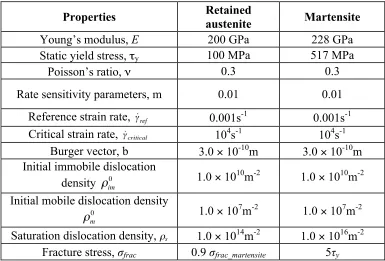
austenite are randomly distributed inside the martensite blocks, or between the blocks and the packets (Figure 4.1). It is assumed that the retained austenite pockets has the same grain orientation as the parent austenite grain. The material properties (Table 4.1) that are used are representative of low-carbon martensitic steel and austenitic stainless steel (Byun et al. 2004).
The parent austenite grain is oriented based on the loading plane of (0 0 1)γ and a loading direction of [0 1 0]γ. The Kurdjumov-Sachs (K-S) OR is adopted as the martensite OR, and {111}γ is assumed as the habit plane. A convergent plane strain FE mesh of 4893 elements was used with a specimen size of 3.2 mm × 6.4 mm, and a displacement load is applied for a quasi-static nominal strain rate with symmetric boundary conditions applied on the left and bottom edges.
4.2 Results and Discussion
4.2.1 Retained Austenite-Martensite Interaction
Different distributions of pockets of retained austenite were randomly distributed within the martensitic aggregate for a volume fraction of 5% (Figure 4.1). It is initially assumed that the austenite grain had a cube Euler orientation of (0º, 0º, 0º). The contours for the normalized (by the initial mobile dislocation density) mobile dislocation densities and the normalized (by the initial immobile dislocation density) immobile dislocation densities corresponding to the most active slip system of the martensite and retained austenite
aggregate at a nominal strain of 20% are shown in Figure 4.3. For the most active slip system
of martensite (112)[1 11], the maximum normalized mobile dislocation density is 2.0 × 10⁷,
and the maximum normalized immobile dislocation density is 1.8 × 10⁵. The evolution of dislocation densities along selected blocks results in the localization of plastic slip (Figure 4.4a). The dislocation density at the interface between martensite blocks and retained austenite pockets is a maximum, and this is likely due to the interaction of the martensitic slip systems and the retained austenite slip systems. Based on the K-S orientation
relationship, the slip systems {110}<111> in martensite should be aligned with the slip systems {111}<110> in austenite. However, the {112}<111> slip systems in martensite are incompatible with the austenite slip systems, which can impede dislocation density
transmission between martensite blocks and retained austenite interfaces. For the most active
slip system in austenite of (1 11)[011], the normalized mobile dislocation density is 2.0 ×
and the lower number of available f.c.c. slip-systems in comparison with the available b.c.c. slip-systems.
The accumulated plastic slip at a nominal strain of 20% is shown in Figure 4.4a. The maximum accumulated slip is 0.5, and it occurs within the retained austenite pockets. The tensile loading direction is aligned along the [010]γ direction, which can result in a maximum resolved shear stress along the [011]γ directions. The slip-direction [011]γ of the f.c.c.
retained austenite is also parallel to the long direction of martensitic laths and blocks, and parallel to the slip direction [111]α based on the K-S OR. The retained austenite grains are at the martensite inter-lath and block boundary, and the long direction should, therefore, be parallel to that of martensite. This would align the austenite slip systems with the maximum resolved shear stress along the long direction of the martensitic blocks and retained austenite grains, which would result in the shear-strain localization of plastic slip. Furthermore, due to
the incompatibility of the b.c.c. slip system (112)[1 11] and the f.c.c. slip system(1 11)[011],
the accumulation of plastic slip occurs at the b.c.c.-f.c.c. interface, which is also exacerbated by the geometrical softening associated with the lattice rotation of both slip-systems (Figure 4.4b).
The interaction density on slip system α, which relates the increase in immobile
dislocation density due to junction formation on the slip system relative to the decrease of mobile dislocation density, can be defined as
ρintrα =
∫
γα gαmnter+ρmα+gimmob+ αb ρim
α
−gmnterα −ρmα−gimmob− α
b ρim
α #
$
%% &
'
which can be used to characterize the dominant interaction mechanism on the active slip systems in the crystalline material. Values of
€
ρintr
α
<0 indicate that the annihilation of
dislocation-density junctions is dominant, while values of
€
ρintr
α
>0 indicate that the formation
of dislocation-density junctions is dominant (Shanthraj and Zikry 2012). The normalized (by the initial immobile dislocation density) total interaction dislocation density at a nominal strain of 20% is shown in Figure 4.4c. The maximum normalized total interaction dislocation density is 1.0 × 10⁵, which occurs in the retained austenite. This indicates that the dominant interaction mechanism in retained austenite is the formation of dislocation junctions, which results in the localization of plastic slip and hardening of retained austenite. The normalized total interaction dislocation density around the periphery of retained austenite pockets in martensite is -1.0 × 10⁴, which indicates that the dominant interaction mechanism is the annihilation of dislocation junctions. This can soften martensite, which can render it more susceptible to shear-strain localization.
4.2.2 Effects of Parent Austenite Orientation
The effects of the initial austenite orientation on the inelastic deformation of the martensite-austenite microstructures have also been investigated. The martensite blocks and retained austenite volume fractions and distributions are the same as before, but the parent austenite Euler angle orientations were varied. Two cases were investigated, one case with a low initial Euler angles of (2º, 4º, 8º), and a second case with a high initial Euler angles of (15º, 25º, 35º).
The contours for the normalized mobile dislocation densities and the normalized immobile dislocation densities corresponding to the most active slip system of martensite and retained austenite, for the Euler angles of (2º, 4º, 8º) at a nominal strain of 20%, are shown in Figure 4.5. The most active slip systems for the martensite blocks and retained austenite pockets are the same as those for the Euler angles (0º, 0º, 0º). For the most active slip system
in martensite of (112)[1 11], the maximum normalized mobile dislocation density is 2.8 ×
107, which is higher than the cube orientation case by approximately 40%. The maximum normalized immobile dislocation density, for the low angle case, is 2.4 × 10⁵, which is 33% higher than the cube case. These larger immobile and mobile dislocation densities are obviously due to the higher incompatibilities of the slip-systems between the retained austenite and the martensite blocks.
case. The maximum lattice rotation is 30º, which is higher than the cube orientation case by approximately 20%. These maximum values occur in the retained austenite regions adjacent to the interface of martensite and retained austenite (Figure 4.6a-c). The higher positive values of the total interaction dislocation density indicate that more dislocation density junctions can form, which results in the hardening of the retained austenite. The maximum normalized normal stress is 20 (Figure 4.6d), and these high stresses are due to the slip system incompatibility between the retained austenite and martensite.
The contours for the normalized mobile dislocation densities and the normalized immobile dislocation densities corresponding to the most active slip system of martensite and retained austenite, for the high Euler angle case at a nominal strain of 20%, are shown in
Figure 4.7. The most active slip system in martensite is(2 11)[11 1], and the most active slip
system in the retained austenite pockets is(1 11)[101], which are not the same as the cube
orientation case and the low Euler angle case.
Some of {110}<111> slip systems in martensite, which are compatible with f.c.c. austenite slip systems, are highly active, as indicated by the high immobile and mobile
in the martensite blocks (Figure 4.8c). This indicates that fewer dislocation-density junctions form in retained austenite, and more dislocation-density junctions are annihilated in
martensite, which can result in shear strain localization and soften the material. The maximum normalized normal stress is 12, and it occurs in the martensitic blocks. The stresses are significantly lower than that of the cube orientation by approximately 14%, and 40% lower than the low Euler angle case. These changes in behavior are due to the
compatibility of the slip systems and the domination of annihilation processes due to dislocation-density interactions at the interface of martensite blocks and retained austenite pockets.
4.2.3 Dynamic Behavior
In this section, we investigate the dynamic behavior of martensitic steel with retained austenite. The martensite blocks and retained austenite volume fractions and distributions are as before, and the parent austenite with a low Euler angle orientation of (2º, 4º, 8º) was used. A displacement load at a steep slope, such that a nominal strain rate of 5000s-1 results along the tensile axis (Figure 4.1). The nominal strain-rate was obtained by scaling the nominal strain over an appropriate time-scale. The nominal stress-strain curves are shown in Figure 4.9. The oscillations at high strain rate occur due to stress wave reflection along the free and fixed boundary.
geometrical softening and thermal softening. The geometrical softening occurs due to large lattice rotations (Figure 4.10b). The maximum value of lattice rotation is 25º. In addition to the geometrical softening, adiabatic heating results in a thermal accumultion (Figure 4.10c). It is assumed in our approach that the thermal accumulation is due to adiabatic heating, and the rate of change of temperature is obtained from the balance of energy (Eq. 2.12). The highest value of normalized temperature is 0.32, and it occurs at the interface of martensite blocks and retained austenite pockets. This increase in temperature further indicates that due to adiabtic heating, the material can soften. These two softening mechanisms would lead to shear strain localization, but it is a material competition with the dynamic strain hardening, which results in large normalized normal stresses of approximately 13 (Figure 4.10d).
4.3 Conclusions
Newly developed dislocation-density based evolution equations are coupled to a multiple-slip crystal plasticity formulation, and a framework is established that relates immobile and mobile dislocation-density evolution to austenitic and martensitic
crystallographic orientations and behavior. Specialized FE methodologies were then used to investigate the effects of retained austenite, parent austenite grain orientations, and quasi-static and dynamic loading rates on deformation and failure in martensitic steel.
For the cube orientation case, the dominant slip system in martensitic blocks
is(112)[1 11], which is incompatible with the retained austenite (f.c.c.) slip systems. The