DOI: 10.1534/genetics.106.061432
Statistical Tests for Detecting Positive Selection by Utilizing
High-Frequency Variants
Kai Zeng,*
,†,1Yun-Xin Fu,
‡,§Suhua Shi* and Chung-I Wu
†*State Key Laboratory of Biocontrol and Key Laboratory of Gene Engineering of the Ministry of Education, Sun Yat-sen University, Guangzhou 510275, China,†Department of Ecology and Evolution, University of Chicago, Chicago, Illinois 60637,‡Human
Genetics Center, School of Public Health, University of Texas, Houston, Texas 77030 and§Laboratory for Conservation and Utilization of Bioresources, Yunnan University, Kunming 650091, China
Manuscript received May 30, 2006 Accepted for publication August 16, 2006
ABSTRACT
By comparing the low-, intermediate-, and high-frequency parts of the frequency spectrum, we gain information on the evolutionary forces that influence the pattern of polymorphism in population samples. We emphasize the high-frequency variants on which positive selection and negative (background) selection exhibit different effects. We propose a new estimator ofu(the product of effective population size and neutral mutation rate),uL, which is sensitive to the changes in high-frequency variants. The new uLallows us to revise Fay and Wu’s H-test by normalization. To complement the existing statistics (the H-test and Tajima’sD-test), we propose a new test, E, which relies on the difference between uL and Watterson’suW. We show that this test is most powerful in detecting the recovery phase after the loss of genetic diversity, which includes the postselective sweep phase. The sensitivities of these tests to (or ro-bustness against) background selection and demographic changes are also considered. Overall,DandHin combination can be most effective in detecting positive selection while being insensitive to other perturbations. We thus propose a joint test, referred to as theDHtest. Simulations indicate that DHis indeed sensitive primarily to directional selection and no other driving forces.
D
ETECTING the footprint of positive selection is an important task in evolutionary genetic studies. Many statistical tests have been proposed for this pur-pose. Some of them use only divergence data between species (see Nei and Kumar 2000 and Yang 2003 for reviews) while others use both divergence and poly-morphism data (for example, Hudson et al. 1987; McDonald and Kreitman 1991; Bustamante et al. 2002). Those that rely only on polymorphism data can be classified into either ‘‘haplotype’’ tests (for example, Hudson et al. 1994; Sabeti et al. 2002; Voight et al. 2006) or the site-by-site ‘‘frequency spectrum’’ tests (for example, Tajima 1989; Fuand Li1993).The frequency spectrum is the distribution of the proportion of sites where the mutant is at frequencyx
and is the focus of this study. We may divide the spectrum broadly into three parts: the low-, intermediate-, and high-frequency variant classes. Comparing the three parts of the spectrum, we shall have a fuller view of the con-figuration of polymorphisms. Tajima’s (1989)Dand Fu and Li’s (1993)Dask whether there are too few or many more rare variants than common ones. Fay and Wu’s (2000) H takes into consideration the abundance of very high-frequency variants relative to the
intermediate-frequency ones. Thus far, there is no test that addresses the relative abundance of the very high- and very low-frequency classes, although this comparison might be the most informative about new mutations. After all, new mutations are most likely to be found in the very low class and least abundant in the very high class.
In this article, we study the power to detect selection by applying spectrum tests to a linked neutral locus. In the first section, we briefly summarize some classical results of the frequency spectrum theory. In the second section, we introduce a new estimator of u(u ¼4Nm, where N is the effective population size and m is the neutral mutation rate of the gene). On the basis of this new estimator, we revise Fay and Wu’sH-test which was not normalized and introduce a new test (E) that con-trasts the high- and low-frequency variants. We further propose a joint test, DH, which is a combination ofD
andH. In the rest of the article, we use computer simu-lation to compare the powers of the tests to detect pos-itive selection. We also consider their sensitivities to balancing selection, background selection, and demo-graphic factors.
GENERAL BACKGROUND
Letjibe the number of segregating sites where the
mutant type occurs i times in the sample. Following Fu (1995), we refer to the class of mutations with i 1Corresponding author:1101 E. 57th St., Chicago, IL 60637.
E-mail: [email protected]
occurrence as mutations of sizei. Given the population mutation rateu, Fu(1995) showed that
EðjiÞ ¼u=i; i¼1;. . .;n1; ð1Þ
for a sample of size n. Since each class of mutations contains information onu, there can be many linear functions of ji that are unbiased estimators of u,
de-pending on how each frequency class is weighted. A general form is
h¼X
n1
i¼1
ciji ð2Þ
withE(h)¼u, whereci’s are weight constants. A few
well-known examples are Watterson’s (1975)uW, Tajima’s (1983) up, Fu and Li’s (1993) je, and Fay and Wu’s
(2000)uH:
uW¼ 1
an Xn1
i¼1 ji;
up¼ n
2 1Xn1
i¼1
iðniÞji;
je¼j1; uH ¼ n
2 1Xn1
i¼1
i2ji; ð3Þ
where an¼Pn 1
i¼1ð1=iÞ. Theoretical variances of these estimators are given in Figure 1. Among them,uWhas the smallest variance.
Different estimators have varying sensitivities to changes in different parts of the frequency spectrum. For example, je and uW are sensitive to changes in low-frequency variants,up to changes in intermediate-frequency var-iants, anduHto high-frequency ones. When the level of variation is influenced by different population genetic
forces, different parts of the spectrum are affected to different extents (Slatkinand Hudson1991; Fu1996, 1997; Fayand Wu2000; Griffiths2003). The difference between twou-estimators can thus be informative about such forces. For example, rapid population growth tends to affect low-frequency variants more than it affects high-frequency ones. As a result,uWtends to be larger thanup. The first test to take advantage of the differences between estimators is Tajima’s D-test (Tajima 1989), as shown below:
D¼ ffiffiffiffiffiffiffiffiffiffiffiffiffiffiffiffiffiffiffiffiffiffiffiffiffiffiffiffiupuW VarðupuWÞ
p : ð4Þ
Others have since been proposed (Fuand Li1993; Fu 1996, 1997; Fayand Wu2000). Among the evolutionary forces that may cause the frequency spectrum to deviate from the neutral equilibrium, hitchhiking (Maynard Smithand Haigh1974) has attracted much attention. A salient feature of positive selection is the excess of high-frequency variants (Fayand Wu2000).
It should be noted thatuWandupcan also be written as
uW ¼s=an; up¼
n
2
1X
i,j
dij; ð5Þ
wheresis the number of segregating sites anddijis the
number of differences between theith andjth sequen-ces. Equation 5 suggests that uW andup can be calcu-lated without using an outgroup sequence to determine the mutant alleles. In contrast, je and uH do require
knowledge of an outgroup sequence. As consequences, Tajima’sDcan be calculated without using an outgroup sequence, while theH-test needs one (see Fu and Li 1993 for a version of Fu and Li’sD-test that usesjebut requires no outgroup sequence in the calculation).
ANALYTICAL RESULTS
Measurements of variation based on very high-frequency variants—uHanduL:To capture the dynam-ics of high-frequency variants, we need to put most weight on high-frequency variants in the estimation of u. Fay and Wu(2000) used uH (3). Its variance term, however, is not easy to obtain. Here we propose a new estimator,uL. The variance ofuLcan be easily obtained and then used to calculate the variance ofuH.
Consider a genealogy ofn genes from a nonrecom-bining region. The mean number of mutations accu-mulated in each gene since the most recent common ancestor (MRCA) of the sample can be calculated as
u9L¼1
n Xn1
i¼1
iji: ð6Þ
SinceE(ji)¼u/i, it follows that
Eðu9LÞ ¼n1
n u: ð7Þ
Although uL9 is an asymptotically unbiased estimator of u, it is more convenient to work with its canonical form
uL¼ 1
n1 Xn1
i¼1
iji; ð8Þ
which hasE(uL)¼u. It can be shown that
VarðuLÞ ¼ n
2ðn1Þu1 2
n n1
2
ðbn111Þ 1
h i
u2;
ð9Þ
wherebn¼
Pn1
i¼1ð1=i
2Þ. Sincei2¼nii(ni), it is easy to see thatuH¼2uLup. From this property, we obtain
VarðuHÞ ¼u1
2½36n2ð2n11Þb
n11116n319n212n3 9nðn1Þ2 u2
ð10Þ
(seeappendix).
The normalized Fay and Wu’sH-statistic—contrasting high- and intermediate-frequency variants:Recall that Fay and Wu’s (2000) His defined asH¼up uH¼ 2(upuL). Now we can write the normalizedH-statistic
as
H ¼ ffiffiffiffiffiffiffiffiffiffiffiffiffiffiffiffiffiffiffiffiffiffiffiffiffiffiffiupuL VarðupuLÞ
p ; ð11Þ
where
VarðupuLÞ ¼
n2 6ðn1Þu
118n
2ð3n12Þb
n11 ð88n319n213n16Þ
9nðn1Þ2 u
2
ð12Þ
(seeappendix). In practice,uin (12) can be estimated by uW, and u2can be estimated by s(s 1)/(a2
n1bn)
(Tajima1989).
A new E-test—contrasting high- and low-frequency variants:As mentioned before, there is no test contrast-ing the low- and high-frequency parts of the spectrum. BothDandHuse intermediate-frequency variants as a benchmark for comparison. Nevertheless, there are oc-casions when it is informative to contrast high- and low-frequency variants. For example, when most variants are lost (e.g., due to selective sweep), the recovery of the neutral equilibrium is most rapid for the low-frequency ones and slowest for the high-frequency ones (e.g., Figure 2B). Taking advantage of the newly deriveduL, we propose a new test statistic
E ¼ ffiffiffiffiffiffiffiffiffiffiffiffiffiffiffiffiffiffiffiffiffiffiffiffiffiffiffiffiuLuW VarðuLuWÞ
p ; ð13Þ
Figure 2.—(A) Changes in RðiÞ ¼Eðj9iÞ=Eðj
iÞ at the linked neutral locus as the advantageous mutation increases in frequency (f). (B) Changes inR(i) at different times t
(measured in units of 4Ngenerations) after fixation of the ad-vantageous mutation. In all simulations, the parameters are defined as follows: u ¼ 4Nm, wherem is the mutation rate for the linked neutral locus; sis the selective coefficient of the advantageous mutation and c is the recombination dis-tance (between the neutral variation under investigation and the advantageous mutation nearby), which is usually scaled by the selective coefficient. The parameter values are
where VarðuLuWÞ
¼ n
2ðn1Þ
1
an
u1 bn a2n12
n n1
2
bn
2ðnbnn11Þ ðn1Þan
3n11
n1
u2
ð14Þ
(see appendix). In practice, u and u2 in (14) can be estimated by methods described after (12). Thus, the three tests, D, H, and E, contrast the three parts of the frequency spectrum, low-, intermediate-, and high-frequency variants, in a pairwise manner. By properly choosing a test statistic, we can have a better chance to detect a particular driving force (e.g., Table 3).
TheDHtest—a jointDandHtest:Simulation results (e.g., Table 3) suggest that bothDandHare powerful in detecting selection, but they are sensitive to different demographic factors and are affected by background selection to different degrees. Therefore, one may con-jecture thatDandHin combination may be sensitive only to selection and less sensitive to other forces. For example, the sensitivity ofD to population expansion may be counterbalanced by the insensitivity ofHto the same factor in the jointDHtest. To carry out the joint
DHtest, we first define
fsðpÞ ¼PfdðXsÞ#dpandhðXsÞ#hpg 0,p,1; ð15Þ whereXsis random samples (of sizen) under neutrality
withs(s$1) segregating sites,d(X) is the value of the
D-statistic of sampleXandh() is that of the normalized
H-statistic, and dp and hp are critical values such that P{d(Xs)#dp}¼P{h(Xs)#hp}¼p. In other words, for a
givens, when the significance levels of bothDandHare
p, that of the jointDHtest isfs(p). That is, for samples
withssegregating sites, the rejection region of theDH
test at the significance level offs(p) is {Xsjd(Xs)#dpand h(Xs)#hp}. In practice, for a given value ofp,fs(p) can be
evaluated using neutral simulations with the number of segregating sitessfixed (Hudson1993). In our
imple-mentation, at least 50,000 rounds of simulations were carried out. To determine a value of p (and conse-quentlydpandhp) such that the significance level ofDH
is, for example, 5%, we solved the equationfs(p)¼0.05
using the bisection algorithm (Press et al. 1992). We denote the solution as p*. We also denote dp and hp
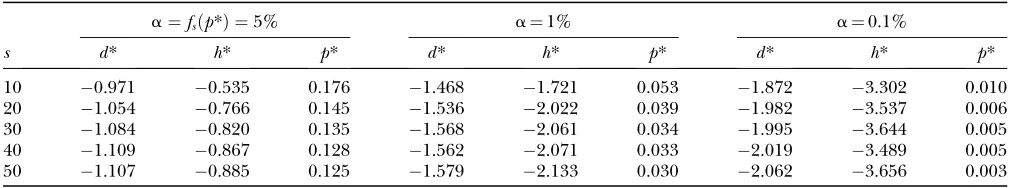
corresponding top* asd* andh*, respectively. In Table 1, we give thep*-,d*-, andh*-values for three significance levels ofDH[i.e.,fs(p*)], given various observed values ofs.
In general,p* is close to three times the value offs(p*).
APPLICATIONS
Here we apply the tests discussed previously to data simulated under a variety of conditions for the purpose of evaluating their statistical powers. Such simulations have been done extensively in the past for studying existing tests (Braverman et al. 1995; Simonsenet al. 1995; Fu 1997; Przeworski2002). Here all tests were one-sided and values falling into the lower 5% tail of the null distribution were considered significant. The reason for the one-sided test is that positive selection predictably shifts the pattern to one side of the null distribution. We report only the results of the normal-izedH-test, because it is always more powerful than the original one (varying from 1 to 8%). Details of the simulation algorithms and other related issues are de-scribed in theappendix.
The power to detect positive selection before and after fixation: For the linked neutral locus, we define
RðiÞ ¼Eðj9iÞ=EðjiÞ, where Eðj9iÞ and EðjiÞ are the
ex-pected numbers of segregating sites of sizeiunder se-lection and neutrality, respectively (Fu 1997). Figure 2 shows the dynamics of R(i) before and after the fix-ation of an advantageous mutfix-ation. The reduction in intermediate-frequency variants and the accumulation of high-frequency variants start at the early stage of the sweep (Figure 2A,f¼0.3;fis the population frequency of the advantageous mutation). When the frequency of the advantageous mutation reaches 60% in the pop-ulation, the spectrum is already highly deviant from neutrality, losing many of the intermediate-frequency
TABLE 1
Critical values of theD- andH-tests (d*andh*) when performed jointly as theDHtest
a¼fsðp*Þ ¼5% a¼1% a¼0.1%
s d* h* p* d* h* p* d* h* p*
10 0.971 0.535 0.176 1.468 1.721 0.053 1.872 3.302 0.010
20 1.054 0.766 0.145 1.536 2.022 0.039 1.982 3.537 0.006
30 1.084 0.820 0.135 1.568 2.061 0.034 1.995 3.644 0.005
40 1.109 0.867 0.128 1.562 2.071 0.033 2.019 3.489 0.005
50 1.107 0.885 0.125 1.579 2.133 0.030 2.062 3.656 0.003
variants (Figure 2A, f ¼0.6). By the time of fixation, the population has lost virtually all the intermediate-frequency variants, and mutations appear at either very high or very low frequency (Figure 2B,t¼0;tis time after fixation of the advantageous mutation and is mea-sured in units of 4N generations). In neutral equilib-rium, there should be 22.4 mutations in the sample on average foru¼5 andn ¼50. However, only 11.4 mu-tations, on average, are seen in the samples at t¼ 0 (Figure 2B), among which 57% have a frequency,10%, and 31% have a frequency.80%. Strikingly, the mean number of mutations of size 49 is 7.2 times that of the neutral expectation. Whent.0, these high-frequency variants quickly drift to fixation and no longer contrib-ute to polymorphism. For a long period after fixation, fewer-than-expected numbers of intermediate- and high-frequency mutations are observed (Figure 2B).
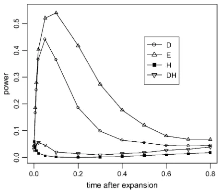
Figure 3 shows how the tests behave before and af-ter the fixation of the advantageous mutation. Before fixation (Figure 3, A and B, left side), the power ofD,
H, and DH increases rapidly as the frequency of the advantageous mutation increases.His generally more powerful than D in this stage. The behavior of DH
resembles that ofH, but note that it is often the most powerful test when the advantageous allele is in high frequency. We should note again that the purpose of the
DHtest is not to increase the power in detecting positive selection over eitherDorHbut to decrease sensitivity to demographical factors and background selection. This is apparent in later sections. In contrast, theE-test has little power. This is expected as the reduction of moderate-frequency variants and the accumulation of high-frequency variants characterize this stage (Figure 2A). Sometimes,H,D, andDHreach their peak of power before fixation. This happens when too much variation is removed by the selective sweep, as is the case in Figure 3A. After fixation (Figure 3, A and B, right side) theE -test quickly becomes the most powerful -test (t0.1 in Figure 3A;t0.15 in Figure 3B). From Figure 2B, we can see that after fixation the low-frequency part of the spectrum recovers first, and the high-frequency part returns to its equilibrium level last. The result of the
E-test fits this observation. Furthermore, since the recovery phase is much longer than the selective phase when selection is strong, the E test can be useful for detecting sweep. TheD-test performs reasonably well in the recovery stage. The power of the H-test, however, decreases quickly. As a consequence, the power of DH
also decreases but at a much lower rate than that ofH. The power to detect balancing selection: Intuition would suggest that the results of an incomplete sweep (Figure 3) may also apply to the initial stage of balancing selection (i.e., a relatively short time period after the birth of the selected allele) under which the selected allele would reach an equilibrium frequency that is high, but ,100%. Furthermore, as the selected allele does not reach fixation, the hitchhiking variants also may not have extreme frequencies. As a result, the sig-nature of positive selection and hitchhiking may linger longer under balancing selection.
Simulation results (see supplemental Figure S1 at http://www.genetics.org/supplemental/) indeed sug-gest that in the phase when the selected allele is ap-proaching the equilibrium frequency (75% in this case), the tests behave very much like the patterns in the left side of Figure 3. After the equilibrium is reached, the powers ofHandDHalso remain higher than in the right side of Figure 3 for a longer period of time. Neverthe-less, the gain is modest as the power to detect selection generally diminishes when the selected allele stops in-creasing in frequency.
Sensitivity of the tests to other driving forces:A good test of a particular population genetic force, say, positive selection, should be sensitive to that force and to that force only. Although a test that is sensitive to many dif-ferent factors can be a useful general tool, it is ultimately uninformative about the true underlying force. Hence, power can in fact be a blessing in disguise. We examine the sensitivity of these tests to forces other than positive selection and balancing selection below.
Figure3.—Power of the tests before and after hitchhiking is completed. Thex-axis on the left represents the increase in the frequency of the advantageous mutation; on the right is the time after fixation (measured in units of 4Ngenerations). All parameter values are the same as those of Figure 2. All tests were one-sided; values falling into the lower 5% tail of the null distribution were considered significant. Results shown in Fig-ures 4–6 were produced by the same method. (A) c/s ¼
Background selection: Selection against linked dele-terious mutations maintained by recurrent mutation, often referred to as background selection, can have ef-fects on the level of genetic diversity similar to those of a selective sweep (Charlesworthet al. 1993). The dis-tinction between selective sweep and background se-lection is therefore crucial. Fortunately, the two modes of selection often have very different effects on the fre-quency spectrum (Fu1997). For example, background selection is not likely to have any effect on high-frequency variants (Fu 1997) and its effect on the low-frequency variants depends onUandN, whereUis the deleterious mutation rate per diploid genome andNis the effective population size.
Table 2 summarizes the power of the tests to detect background selection. BothDandEare sensitive, butD
is slightly more powerful thanE. In general, the power increases asUincreases, but this increase also depends onN. For a givenU, the power of the tests decreases as
N increases. H is not affected in all cases and hence is discriminatory between the two modes of selection. Significantly,DHis also not sensitive to background se-lection. It seems that the sensitivity ofDis well count-erbalanced by the insensitivity ofH.
Population growth: When a population increases in size, it tends to have an excess of low-frequency variants (Slatkinand Hudson1991; Fu1997; Griffiths2003). Both D and E are sensitive to this type of deviation (Figure 4). E is the most sensitive test because high-frequency variants are the last to reach the new equi-librium after expansion. In contrast, H is unaffected. Strikingly,DHhas little power in this case even though
Dexhibits tremendous power.
Population shrinkage: When the population de-creases in size, the number of low-frequency variants tends to be smaller than that of the intermediate- and high-frequency ones (Fu1996). Thus,Hcan be sensitive to population shrinkage, whereas D, E, and DH are largely unaffected (Figure 5).
TABLE 2
Powers ofD,E,H, andDHto detect background selection
U N u D E H DH
0.01 2,500 1 0.06 0.05 0.04 0.04 10 0.06 0.06 0.05 0.05 50,000 1 0.05 0.04 0.05 0.04 10 0.05 0.06 0.05 0.06
0.1 2,500 1 0.08 0.02 0.04 0.01
10 0.34 0.34 0.02 0.09 5,000 1 0.06 0.01 0.04 0.01 10 0.23 0.23 0.03 0.06 10,000 1 0.04 0.00 0.04 0.01 10 0.15 0.14 0.03 0.06 20,000 1 0.02 0.00 0.04 0.00 10 0.11 0.10 0.04 0.05 50,000 1 0.02 0.00 0.05 0.00 10 0.07 0.06 0.05 0.04
0.2 2,500 1 0.09 0.02 0.02 0.01
10 0.60 0.55 0.02 0.07 5,000 1 0.07 0.00 0.02 0.00 10 0.47 0.35 0.03 0.05 10,000 1 0.04 0.00 0.03 0.00 10 0.35 0.18 0.02 0.03 20,000 1 0.02 0.00 0.03 0.00 10 0.21 0.08 0.03 0.02 50,000 1 0.02 0.00 0.01 0.00 10 0.11 0.02 0.03 0.01
Sample size is 50. A total of 5000 samples were simulated for each parameter set. All runs employed values of h (domi-nance coefficient) and s (selection coefficient) of 0.2 and 0.1;i.e.,sh¼0.02.Uis the deleterious mutation rate per dip-loid genome.Nis the effective population size.
Figure4.—Sensitivity (or power) of the tests to population expansion. We assume that the effective population size in-creases 10-fold instantaneously at time 0 tou¼5. Sample size (n) is 50. Time is measured in units of 4Ngenerations.
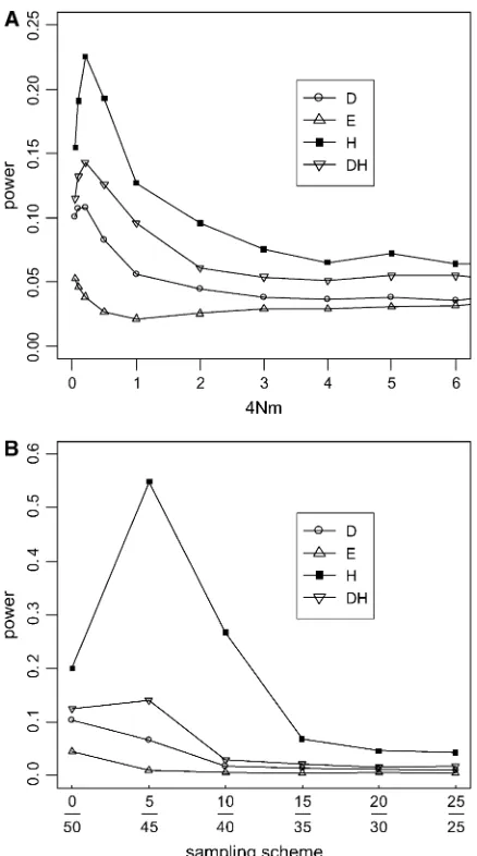
Population subdivision:When the population is struc-tured, one commonly uses the fixation index FSTas a measure of genetic differences among subpopulations. In the symmetric two-deme model,FST¼1/(1116Nm), wheremis the fraction of new migrants in the popula-tion andNis the population size of a deme (Nordborg 1997). When there is strong population subdivision (FST.0.2 or 4Nm,1, for example) and samples do not come equally from all subpopulations, the frequency spectrum is deviant from the neutral equilibrium (re-sults not shown). Figure 6A gives an example where all
genes are taken from one subpopulation. In this case,
His the most sensitive test. TheD-test is sensitive only when the subdivision is strong (4Nm , 0.5 or FST . 0.33).DHhas some sensitivity. Its power lies in between those ofDandH, but never rises above 15%. Note that, for relatively mild population subdivisions with 4Nm.
2, none of these four tests is notably affected. Interest-ingly, E is completely insensitive to population subdi-vision. Figure 6B shows the effect of sampling on the power of the tests (4Nm¼0.1). TheE-test again shows no sensitivity. Although the power ofHcan be as high as 55%, that of the DH test never goes above 14%. This result shows the effectiveness of usingDandHin com-bination. However, when sampling becomes less and less biased, all tests become progressively less sensitive to population structure.
CONCLUSION
We summarize our results in Table 3. It is clear that, among the four tests studied,DHis sensitive primarily to directional selection. In contrast, other tests are sensitive to two or more other driving forces.Dis indeed a ‘‘gen-eral purpose’’ test as it is sensitive, to various extents, to all the processes we considered (Table 3). Being exclu-sive is a desirable property because it minimizes false positive results in the search for selectively favored mu-tations. However, no test is powerful in every stage of the selection process. Therefore, in practice, we should utilize a priori information (if available) from other sources to help us choose an appropriate test.
We thank J. Braverman and R. R. Hudson for their helpful dis-cussions about the simulation algorithms. We also thank two anony-mous reviewers for their constructive comments. K.Z. is supported by Sun Yat-sen University and the Kaisi Fund. S.S. is supported by grants
Figure6.—Sensitivity (or power) of the tests to population subdivision. A symmetric two-deme model with u ¼ 2 per deme (2N genes per deme) was simulated. Populations are assumed to be in drift–migration equilibrium with symmetric migration at a rate ofm, which is the fraction of new migrants each generation. Sample size (n) is 50. (A) Sensitivity as a function of the degree of population subdivision, expressed as 4Nmon thex-axis. All genes were sampled from one sub-population. (B) Sensitivity as a function of the sampling skew-ness; for example, 5/45 means 5 genes are sampled from one subpopulation and 45 from the other. In this case, 4Nm¼0.1, a value at which the tests show sensitivity to population sub-division in A.
TABLE 3
A qualitative summary of the powers of the four tests to detect various population genetic forces
Driving force D H E DH
Positive selection (before fixation)
111 111 111
Positive selection (after fixation)
111 11 111 11
Balancing selection (initial stage)
11 111 111
Background selection 11 11
Population growth 111 111
Population shrinkage 1 11 1
Subdivision 1 11 1
The results were drawn on the basis of Figures 3–6 and Table 2. All tests were one-sided; values falling into the lower 5% tail of the null distribution were considered significant.
denotes the lack of power under the specified condition.
from the National Natural Science Foundation of China (30230030, 30470119, 30300033, and 30500049). Y.-X. Fu is supported by National Institutes of Health (NIH) grants (GM 60777 and GM50428) and funding from Yunnan University, China. C.-I Wu is supported by NIH grants and an OOCS grant from the Chinese Academy of Sciences.
LITERATURE CITED
Braverman, J. M., R. R. Hudson, N. L. Kaplan, C. H. Langleyand
W. Stephan, 1995 The hitchhiking effect on the site frequency
spectrum of DNA polymorphisms. Genetics140:783–796. Bustamante, C. D., R. Nielsen, S. A. Sawyer, K. M. Olsen, M. D.
Puruggananet al., 2002 The cost of inbreeding inArabidopsis.
Nature416:531–534.
Charlesworth, B., M. T. Morganand D. Charlesworth, 1993 The
effect of deleterious mutations on neutral molecular variation. Genetics134:1289–1303.
Charlesworth, D., B. Charlesworth and M. T. Morgan, 1995
The pattern of neutral molecular variation under the back-ground selection model. Genetics141:1619–1632.
Fay, J. C., and C.-I Wu, 2000 Hitchhiking under positive Darwinian
selection. Genetics155:1405–1413.
Fu, Y. X., 1995 Statistical properties of segregating sites. Theor.
Popul. Biol.48:172–197.
Fu, Y. X., 1996 New statistical tests of neutrality for DNA samples
from a population. Genetics143:557–570.
Fu, Y. X., 1997 Statistical tests of neutrality of mutations against
pop-ulation growth, hitchhiking and background selection. Genetics 147:915–925.
Fu, Y. X., and W. H. Li, 1993 Statistical tests of neutrality of
muta-tions. Genetics133:693–709.
Griffiths, R. C., 2003 The frequency spectrum of a mutation, and its
age, in a general diffusion model. Theor. Popul. Biol.64:241–251. Hudson, R. R., 1993 The how and why of generating gene
geneal-ogies, pp. 23–36 inMechanisms of Molecular Evolution, edited by N. Takahataand A. G. Clark. Sinauer, Sunderland, MA.
Hudson, R. R., 2002 Generating samples under a Wright-Fisher
neutral model of genetic variation. Bioinformatics18:337–338. Hudson, R. R., and N. L. Kaplan, 1994 Gene trees with background
selection, pp. 140–153 inNon-Neutral Evolution: Theories and Mo-lecular Data, edited by B. Golding. Chapman & Hall, London.
Hudson, R. R., M. Kreitmanand M. Aguade´, 1987 A test of neutral
molecular evolution based on nucleotide data. Genetics 116: 153–159.
Hudson, R. R., K. Bailey, D. Skarecky, J. Kwiatowski and F. J.
Ayala, 1994 Evidence for positive selection in the superoxide
dismutase (sod) region ofDrosophila melanogaster. Genetics136: 1329–1340.
Kaplan, N. L., R. R. Hudsonand C. H. Langley, 1989 The
‘‘hitch-hiking effect’’ revisited. Genetics123:887–899.
Markovtsova, L., P. Marjoramand S. Tavare´, 2001 On a test of
Depaulis and Veuille. Mol. Biol. Evol.18:1132–1133.
MaynardSmith, J., and J. Haigh, 1974 The hitch-hiking effect of a
favourable gene. Genet. Res.23:23–35.
McDonald, J. H., and M. Kreitman, 1991 Adaptive protein
evolu-tion at theadhlocus inDrosophila. Nature351:652–654. Nei, M., and S. Kumar, 2000 Molecular Evolution and Phylogenetics.
Oxford University Press, New York.
Nordborg, M., 1997 Structured coalescent processes on different
time scales. Genetics146:1501–1514.
Press, W. H., S. A. Teukolsky, W. T. Vetterlingand B. P. Flannery,
1992 Numerical Recipes in C: The Art of Scientific Computing. Cambridge University Press, Cambridge, UK.
Przeworski, M., 2002 The signature of positive selection at
ran-domly chosen loci. Genetics160:1179–1189.
Sabeti, P. C., D. E. Reich, J. M. Higgins, H. Z. Levine, D. J. Richter
et al., 2002 Detecting recent positive selection in the human genome from haplotype structure. Nature419:832–837. Simonsen, K. L., G. A. Churchilland C. F. Aquadro, 1995
Prop-erties of statistical tests of neutrality for DNA polymorphism data. Genetics141:413–429.
Slatkin, M., and R. R. Hudson, 1991 Pairwise comparisons of
mi-tochondrial DNA sequences in stable and exponentially growing populations. Genetics129:555–562.
Stephan, W., T. H. E. Wieheand M. W. Lenz, 1992 The effect of
strongly selected substitutions on neutral polymorphism - analyt-ical results based on diffusion-theory. Theor. Popul. Biol. 41: 237–254.
Tajima, F., 1983 Evolutionary relationship of DNA sequences in
fi-nite populations. Genetics105:437–460.
Tajima, F., 1989 Statistical method for testing the neutral mutation
hypothesis by DNA polymorphism. Genetics123:585–595. Voight, B. F., S. Kudaravalli, X. Wenand J. K. Pritchard, 2006 A
map of recent positive selection in the human genome. PLoS Biol.4:e72.
Wall, J. D., and R. R. Hudson, 2001 Coalescent simulations and
sta-tistical tests of neutrality. Mol. Biol. Evol.18:1134–1135. Watterson, G. A., 1975 On the number of segregating sites in
ge-netical models without recombination. Theor. Popul. Biol. 7: 256–276.
Yang, Z., 2003 Adaptive molecular evolution, pp. 229–254 in
Hand-book of Statistical Genetics, edited by D. Balding, M. Bishopand
C. Cannings. Wiley, New York.
Communicating editor: N. Takahata
APPENDIX
Analytical results: We list some useful properties of the u-estimators (see Y.-X. Fu, unpublished data, for mathematical details):
Covðup;uLÞ ¼ n11 3ðn1Þu1
7n213n24nðn11Þb
n11 2ðn1Þ2 u2;
CovðuL;uWÞ ¼
u an
1nbnn11 anðn1Þ
u2: ðA1Þ
SinceuH ¼2uLup, using (A1), we have
VarðuHÞ ¼u1
2 36n2ð2n11Þbn11116n319n212n3
9nðn1Þ2 u
2:
ðA2Þ
VarðupuLÞand VarðuLuWÞcan be calculated using the above formulas.
recombination distance between the selective locus and the neutral locus (c) was a given value rather than a random variable.
We extended the coalescent simulation algorithm described above to incorporate the case of incomplete hitchhiking. Suppose that the frequency of the favored allele isf. By solving the deterministic equation given by Stephanet al. (1992; Equation 1 in Bravermanet al. 1995), one may obtain the time since the birth of this advantageous mutation and the corresponding fre-quency trajectory. In each replicate of simulation, we assigned the number of genes linked to the advanta-geous allele by binomial sampling with parameters n
andf. Then the genealogy was constructed following the same procedure as described above.
Background selection and demographic scenarios:We sim-ulated background selection using the coalescent method (Hudsonand Kaplan1994; Charlesworthet al. 1995). The software package kindly provided by Hudson (2002) was used to simulate all demographic scenarios.