NONLINEAR TIME-DOMAIN SOIL-STRUCTURE INTERACTION
ANALYSIS OF EMBEDDED REACTOR STRUCTURES SUBJECTED TO
EARTHQUAKE LOADS
Jerome M. Solberg1, Quazi Hossain2
1 Methods Development Group, Lawrence Livermore Nat’l Lab, Livermore, CA ([email protected]) 2 Structural and Applied Mechanics Group, Lawrence Livermore Nat’l Lab, Livermore, CA
ABSTRACT
A generalized time-domain method for Soil-Structure Interaction Analysis is developed, based upon an extension of the Bielak Method. The methodology is combined with the use of a simple hysteretic soil model based upon the Ramberg-Osgood formulation and applied to a notional Small Modular Reactor. These benchmark results compare well with those obtained by using the industry-standard frequency-domain code SASSI. The methodology provides a path forward for investigation of other sources of nonlinearity, including those associated with the use of more physically-realistic material models incorporating pore-pressure effects, gap opening/closing, the effect of nonlinear structural elements, and 3D seismic inputs.
INTRODUCTION
For over 30 years, modeling of nuclear power reactors for seismic safety has been conducted using a simplified soil-structure interaction (SSI) analysis approach that has proven remarkably powerful given the then available knowledge of the response of structures, soils, and their interactions under the cyclical loading of seismic shaking. This analysis approach is exemplified by the computer program SASSI, which has been subject to continuous improvement since its introduction in the early 1980’s, see Ostadan (2007). However, many of the inherent limitations of the overall approach remain.
Technology related to earthquake rupture, seismic wave propagation, structural mechanics, and soil models have all advanced enormously since the early eighties, grounded substantially on the rapid advance in computing power. Much more robust models are now available to address each part of power reactor seismic response (source to site) and to address all of the relevant physics including nonlinear features of site and structure response. Given recent events in which nuclear power reactors have been subjected to beyond-design seismic shaking, as well as the emergence of advanced reactor designs, an important and urgent question is whether a coherent new approach incorporating advanced nonlinear models and modeling techniques using high performance computing can predict nuclear reactor response to earthquakes with higher fidelity than standard techniques in current use.
THE NEED FOR NON-LINEAR TIME DOMAIN ANALYSES
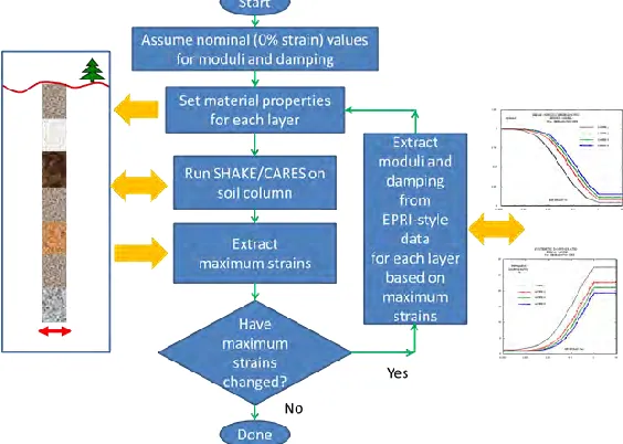
The current approach as represented by the computer code SASSI solves the equations of motion in the frequency-domain. Such an approach is inherently limited to linear representation of soil properties as it relies on the principle of superposition. Soils are strongly nonlinear even at small strains, featuring both strain-dependent stiffness and strain-dependent damping characteristics, as documented for example in the EPRI report on strain-dependent soil characteristics, see EPRI (1993) and Figure 1. SASSI can incorporate these strain dependencies only indirectly, via the equivalent-linear approach, see Figure 2. Soils typically exhibit stiffness and damping properties that are significantly affected by changes in three-dimensional confining pressures as the seismic event progresses, see Zhang, Andrus and Juang (2005). Many soils typically exhibit significant evolution of the soil response over a number of strain cycles, often in concert with pore water pressure and content evolution, see Matasovic and Vucetic (1993). The current SASSI approach is not capable of incorporating these latter two effects, even indirectly.
In the equivalent-linear method used by SASSI, the maximum strains as a function of vertical position in the soil column are estimated for a specified seismic input via a 1D soil column solution (without the structure) performed by a code such as SHAKE, see Idriss, Sun, Schnabel, Lysmer, and Seed (1992) or CARES, see
Costantino, Miller and Xu (1995).
Constant stiffness and damping values are selected for each soil layer based upon this prediction and utilized in the SASSI calculation. This method may be non-conservative in a number of cases: It may underpredict the response in regions with low (but significant) amplitude response, as often occurs at higher frequencies, see Assimaki and Kausel (2002).
It may underpredict deformation at locations of local stress concentrations, where softening in excess of that predicted may occur, see Bonilla, Archuleta and Lavallee (2005).
It cannot account for the pressure dependence of soils, see Zerfa and Loret (2003), an effect that is particularly important in the presence of “raft uplift” that may occur under portions of the basemat during rocking motions, see Wolf and Song (2002).
The “hysteretic damping” used in equivalent-linear analyses, although perhaps better able to model certain experimental results than simple Kelvin-Vogt models typically used in linear time-domain analysis, is mathematically suspect since it cannot be transformed to a causal function in the time-domain, see Crandall (1970).
Equivalent-linear analyses cannot account for geometric nonlinearity resulting from separation (contact/release) at the interface between the soil and the structure during a seismic event.
Figure 1 - Typical Shear Modulus Degradation and Damping Curves
Figure 2 - Calculation of Equivalent-Linear Properties
THE BIELAK METHOD AND THE EXTENSION TO NONLINEAR MATERIALS
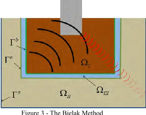
To develop a state-of-the-art nonlinear time-domain SSI analysis method, LLNL started with, and extended, a method developed by Bielak and coworkers, see Bielak, Loukakis, Hisada and Yoshimura (2003). The Bielak method (see Figure 3) provides a rational means for applying seismic input motion. The method consists of two primary steps:
1) Partition the soil around the building into three regions, ΩI (the inner region immediately around
the building), ΩII (the outer region that prevents wave reflection), and ΩIII (the intermediate
region), as shown in Figure 3.
2) Drive the inner region ΩI according to a prescribed seismic input time history, through forces
applied in the intermediate region ΩIII. Assuming the seismic input time history is consistent with
the discrete solution in ΩI (absent the structure), the motion in the outer region ΩII consists only
of the waves scattered by the presence of the structure. This algorithm has the following key features:
2) In the absence of the structure, the exact solution for the seismic wave is reproduced within ΩI
and zero displacement is recovered within ΩII (assuming the seismic input corresponds to the
exact solution for a seismic wave within ΩII).
3) The need for a high-performance absorbing boundary is greatly reduced, since
a. The seismic input does not require an absorbing boundary condition to be “driven backwards”, since the seismic input is realized using another technique.
b. The only waves that propagate within ΩII are the scattered waves, which are of
significantly reduced magnitude in comparison to the seismic input.
c. As the material response within ΩII may include dissipation, and as a result of geometric
attenuation, the magnitude of the scattered waves by the time they reach the outer boundary is small, even when compared with the magnitude at the structure (the source of the scattered waves).
Figure 3 - The Bielak Method
The Bielak method assumes the existence of an exact solution u u x ( , )t
for the displacement
u
in a free-field wave propagation problem as a function of position xand time
t
. Via standard kinematics,the symmetric small strain tensor su
and its time derivative
suare also known throughout the
domain as a function of time and position.
Through the constitutive relation of the material, the exact solution thence gives rise to an exact solution for the Cauchy stress σ σ x ( , )t,
see Equation 1(1)
In the original Bielak method, the region ΩIII is assumed one element thick. Therefore, the nodes
associated with elements in ΩIII fall into two categories, those associated with the “seismic input”
boundaryb
, and those associated with the boundary with ΩII , 0 as in Figure 3. Construct a smooth
non-negative scalar function B( )x with value 1 on b and value 0 on0
, see Equation 2:
(2)
0
1
( ) :
0
b
B
x
x
x
( , )
( , )
( , )
(
s,
s)
( , )
t
t
t
t
The scaling function is used to produce a scaled solution u x( , )t
and the resulting Cauchy Stress
( , )t
σ x within ΩIII, Equation 3:
(3)
For nodes with (vector) shape function Nnode that are located on 0, or entirely within the region
ΩIII , the vector of nodal forces
F
node due to the scaled solution are subtracted from the current solution.For nodes that are located in
b, the nodal forces
F node due to the scaled solution are subtracted, andthen those from the exact solution are added (as evaluated within ΩIII ). In other words, the nodal forces
resulting from elements within ΩIII are calculated according to Equation 4:
(4)
In the absence of scattered waves from the structure, the following solution (Equation 5) is recovered, where it is noted that the solution is zero in the external region
II(5)
If scattered waves are generated by the structure, they will perturb the solution everywhere, thus inducing non-zero solutions within ΩII. However, the scattered waves will be generally significantly
smaller in magnitude than the incident waves. In addition, because of material dissipation and geometric attenuation, by the time these waves reach the external boundary, their magnitude will be reduced further. Hence the absorbing boundary condition need not be exceptionally effective at attenuating reflections at the external boundary.
Bielak and coworkers developed their original method for linear materials in matrix form, assuming the intermediate region is one element thick. Equation 5 recovers the Bielak solution for linear materials, but is valid equally for non-linear materials and for an intermediate region which is more than one element thick, assuming the scaling functionB( )x defined in Equation 2 is defined smoothly
within
the interior of
ΩIII. However, an additional modification to the method is necessary for nonlinearmaterials. A nonlinear material has variable impedance (the tangent modulus varies as a function of strain level and strain history). For soils, the impedance at large strains is typically lower than the impedance at zero strain. In order to ensure that waves reflected by the structure do not reflect at the layer boundaries, the impedance within ΩIII should vary smoothly from the high-impedance value of the
undisturbed soil in ΩII to the low-impedance value of the highly strained soil within ΩI. This principle is
illustrated in Figure 4.
( , )
( ) ( , )
(
s,
s)
( , )
t
t
t
u x
x u x
σ σ u u σ x
( , ) ( , ) ( , ) ( , ) ( , ) ( , ) I I III III II II t t
x t t x t t
u x x σ x x
u u x x σ σ x x
0 x 0 x
node is NOT located on
node IS located on
b III
b III
S node node
node
S node node
d d
σ σ N u u N
F
Figure 4 - Required variation of impedance within the intermediate region
Unfortunately, the strain which is developed within ΩIII by the scaled solution of Equation 3 does
not lead to smoothly varying impedance, as the strain contains an extra term due to the gradient of
( )x,
that is
(6)
The extra term leads to increased strain (and stress) in the intermediate layer, which may lead to deleterious effects. To first order, the impedance may suffer a jump at the interfaces b and0. More
seriously, more complex material models (incorporating, for example, pressure dependency) may fail if the material experiences tension – which may be induced by this second term. Therefore, the following modification to the strain and strain rate is used within the intermediate layer:
(7)
Incorporating this modified strain produces strains (and hence stresses and impedances) which vary smoothly within the intermediate layer and across the layer boundaries.
COMPARSION WITH CARES/SASSI
For comparison with the current state-of-the-art, the soil was represented by a 3D extension of the simple nonlinear hysteretic Ramberg-Osgood material model, see Ramberg and Osgood (1943). The Ramberg-Osgood model requires the determination of four parameters to fit the behavior of each of the 9 soil layers, using an algorithm (RAMBO) developed earlier at LLNL, see Ueng and Chen (1992). Soil parameters were based on an existing site response analysis for 9 soil layers extracted from a deep soil location at the DOE Savannah River Site, see Wyatt and Harris (2004). Typical fits of the Ramberg-Osgood model versus the data are presented in terms of soil degradation and damping curves as Figure 5.
( , )
( ) ( , )
( )
Ss s
t
t
u x
x u x
u
x
u u
ˆ( ) ( , ) ˆ( ) ( , )
s
s s
s
s s
t
t
ε u u x u
Figure 5 - Typical Ramberg-Osgood fits versus data
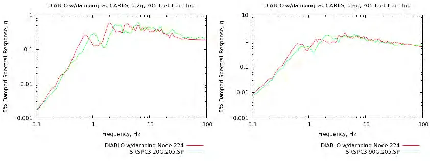
These same soil parameters were utilized by Professor Carl Costantino within the 1-D Soil Column simulator CARES, see Costantino, Miller and Xu (1995), and used to extract equivalent-linear soil properties and predicted motions for notional 0.2g, 0.5g, and 0.9g earthquakes. In contrast to the equivalent-linear approach, the parameters for the Ramberg-Osgood model were only fit once, since they depend only on the soil data and not on the particular earthquake. As the Ramberg-Osgood model cannot produce damping all the way down to zero strain, it was necessary to introduce a small amount of damping (1.5% of critical at 1 and 30 Hz) to provide a good match to the response predicted by CARES. Typical comparisons of 5% damped response spectra (5% damped harmonic oscillator subjected to the acceleration time history, max acceleration versus oscillator natural frequency) are provided as Figure 6, where the left hand figure represents the response to a 0.2g earthquake at a position 205 feet from the top of the soil column, and the right hand figure represents the response at the same location to a 0.9g earthquake. Note the excellent match, especially at the 0.9g earthquake level – in both instances the peak frequencies are shifted somewhat with respect to CARES, more prominently in the 0.2g case.
Figure 6 - Typical comparisons of DIABLO versus CARES, 5% damped response spectra
effects of equipment, as well as a section of the second floor with a greatly increased floor weight, representing the presence of a water tank. The reactor model was embedded in a layered soil domain with layer properties and spacing as in the 1D soil column analysis (see Figure 7, right) and the entire model (soil and reactor) subjected to the notional 0.2g, 0.5g, and 0.9g earthquake loads, represented as vertically propagating shear waves.
Figure 7 - Notional Small Modular Reactor, with outer walls removed (left), and with outer walls and piers removed (center), and embedded within layered soil (right)
The DIABLO analysis using the Ramberg-Osgood material model and the modified Bielak method was compared to SASSI analysis performed by Brookhaven National Laboratory using the equivalent-linear material properties as determined by the aforementioned CARES analysis. The solution was compared at selected points in the reactor structure both in terms of maximum acceleration (see Figure 8) and via 5% damped response spectra (see Figure 9).
Close examination of Figure 8 shows a good match of the peak accelerations versus SASSI. Typically peak response match is worst at the larger earthquake levels, for which differences in material response are likely to be accentuated. Generally speaking, DIABLO has lower peak acceleration than SASSI at these higher earthquake levels, but this trend does not hold in all cases.
Figure 8 - Comparison of peak acceleration, SASSI (open bars) versus DIABLO (solid bars), at various locations along the structure centerline, for earthquake levels 0.2g (green), 0.5g (blue), and 0.9g (red)
probably due to the reduced damping and higher modulus at low strain levels (in comparison to SASSI, which has fixed modulus and strain for each earthquake level) utilized in the Ramberg-Osgood model within DIABLO, supported by the observation that the Z-component match becomes progressively worse as the earthquake level increases, where SASSI would have further reduced modulus and increased damping. As was the case for the comparison with the 1D soil column data, the response in the X-direction matches well, but with peak values shifted to lower frequencies for DIABLO.
Figure 9 - 5% damped response spectra, DIABLO(red) v. SASSI(black), various earthquake levels, basemat center
SUMMARY AND CONCLUSION
REFERENCES
Assimaki, D., and Kausel, E. (2002). "An equivalent linear algorithm with frequency- and pressure-dependent moduli and damping for the seismological analysis of deep sites". Soil Dynamics and
Earthquake Engineering, 22, 950-965.
Bielak, J., Loukakis, K., Hisada, Y. and Yoshimura, C. (2003, April). "Domain Reduction Method for Three-Dimensional Earthquake Modeling in Localized Regions, Part I: Theory". Bulletin of the
Seismological Society of America, 93(No. 2), 817–824.
Bonilla, L. F., Archuleta, R. J., and Lavallee, D. (2005, December). "Hysteretic and Dilatant Behavior of Cohesionless Soils and Their Effects on Nonlinear Site Response: Field Data Observations and Modeling". Bulletin of the Seismological Society of America, 95(6), 2373–2395.
Costantino, C. J., Miller, C., and Xu, J. (1995). CARES: Computer Analysis for Rapid Evaluation of
Structures Version 1.2. Monsey, N.Y.: Constantino, Miller and Associates.
Crandall, S. H. (1970). "The Role of Damping in Vibration Theory". Journal of Sound and Vibration, 11(1), 3-18.
Drosos, V. A., Gerolymos, N., and Gazetas, G. (2012). "Constitutive model for soil amplification of ground shaking: Parameter calibration, comparisons, validation". Soil Dynamics and Earthquake
Engineerg, 42, 255-274.
EPRI. (1993). Guidelines for determining design basis ground motions, Final Report. Electric Power Research Institute (EPRI).
Idriss, I. M., Sun, J. I., Schnabel, P., Lysmer, J., and Seed, H. B. (1992). Users Manual for SHAKE 91, A Computer Program for Conductiving Equivalent Linear Seismic Response Analyses of
Horizontally Layered Soil Deposits. Building and Fire Research Laboratory,, Structures Division.
Gainsville, Maryland: National Institute of Standards.
Matasovic, N. and Vucetic, M. (1993, November). "Cyclic Characterization of Liquifiable Sands".
Journal of Geotechnical Engineering, 119(11), 1805-1822.
Ostadan, F. (2007, April). SASSI 2000 User's Manual, Version 3.
Ramberg, W., and Osgood, W. R. (1943). Description of Stress-strain curves by three parameters. National Advisory Committee for Aeronautics, USA (NACA).
Soga, K. and O'Sullian, C. (2010, December). "Modeling of Geomaterials Behavior". Soils and
Foundations, 50(6), 861-875.
Solberg, J. M., Hossain, Q., Blink, J. A., Bohlen, S., Mseis, G., and Greenberg, H. (2013). Development of a Generalized Methodology for Soil-Structure Interaction Analysis Using Nonlinear
Time-Domain Techniques - NEAMS Program, DOE Office of Nuclear Energy (NE-41) . Lawrence
Livermore National Laboratory.
Ueng, T.-S. and Chen, J.-C. (1992). Computational Procedures for Determining Parameters in
Ramberg-Osgood Elastoplastic Model Based on Modulus and Damping versus Strain. Lawrence Livermore
National Laboratory. Livermore, CA: Lawrence Livermore National Security.
Wolf, J. P. and Song, C. (2002). "Some cornerstones of dynamic soil–structure interaction". Engineering
Structures, 24, 13-28.
Wyatt, D. E. and Harris, M. K. (2004, December). "Overview of the history and geology of the Savannah River Site". Environmental Geosciences, 11(4), 181-190.
Zerfa, F. Z. and Loret, B. (2003). "Coupled dynamic elastic–plastic analysis of earth structures". Soil
Dynamics and Earthquake Engineering, 23, 435–454.