ABSTRACT
CHEN, JIANJUN. Optimization of Cost and Emissions of a KRW-Gasifier based IGCC System under Variability and Uncertainty (Under the supervision of Dr. H.C. Frey).
of a KRW-Gasifer based IGCC system when both variability and uncertainty in model parameters are considered.
The methodologies proposed and demonstrated in this study are helpful to design and evaluation of advanced technology applications where cost minimization, risk analysis, environmental compliance and R&D priority remain important issue.
OPTIMIZATION OF COST AND EMISSIONS OF A KRW-GASIFIER
BASED IGCC SYSTEM UNDER VARIABILITY AND UNCERTAINTY
by
JIANJUN CHEN
A thesis submitted to the Graduate Faculty of North Carolina State University
in partial fulfillment of the requirements for the Degree of
Master of Science
DEPARTMENT OF CIVIL, CONSTRUCTION AND
ENVIRONMENTAL ENGINEERING
Raleigh 2003
APPROVED BY
BIOGRAPHY
ACKNOWLEDGEMENT
First of all, I want to thank Dr. Frey, my advisor, for providing me with a research assistantship. Study under Dr. Frey’s guidance was stimulating and also joyful. I am particularly excited about being given chance to work on modeling vehicle emissions. Meanwhile, I take this opportunity to thank Dr. Frey’s support and patience during my long vacation at China (Due to visa problem). I would also like to express my thanks to other two committee members: Dr. Ranjithan and Dr. Brill for their time and helps.
I want to extend my appreciation to other people in Dr. Frey’s research group. They are: Allen, Alper, Amir, Kaishan, Maggie, Minsheng, Yunhua, and Tanwir. Particularly, to Allen for going through my thesis again and again; to Alper for sharing me with his knowledge and experiences in vehicle emissions; to Kaishan for many helps which made it possible that I can work partly at home when I was waiting for visa. Specially, I am indebted to Minsheng. My life here became much easier thanks to his kind and generous helps during the past two years.
I am grateful to my families: my father and mother, younger brother and others, for their love, support and sacrifice made to allow me keeping staying at schools (Unfortunately, I will spend probably another four years in school).
TABLE OF CONTENTS
LIST OF TABLES ...vi
LIST OF FIGURES ...ix
1.0 INTRODUCTION... 1
2.0 CONCEPT AND METHODOLOGY ... 5
2.1 Variability and Uncertainty... 5
2.2 Sampling Technique for Variability and Uncertainty... 6
2.3 Stochastic Optimization and Stochastic Programming... 9
2.3.1 Stochastic Optimization... 9
2.3.2 Stochastic Programming ... 12
2.4 Optimization Considering both Variability and Uncertainty... 13
3.0 OVERVIEW OF INTEGRATED GASIFICATION COMBINED CYCLE (IGCC) SYSTEM ... 20
3.1 Performance, Emissions and Cost Model for KRW Gasifier-based IGCC System... 22
3.2 Interface of the Model... 24
3.3 Variability and Uncertainty in Model Inputs ... 25
4.0 SOFTWARE IMPLEMENTATION ... 34
4.1 Random Number Generator... 34
4.2 Overview of the Optimizer ... 34
4.2.1 Overview of Genetic Algorithms... 35
4.2.2 Overview of Evolver... 38
4.2.3 Performance of GA in Optimization of Process Models ... 39
4.3 Software Organization ... 43
5.0 CASE STUDY OF OPTIMIZATION UNDER VARIABILITY AND UNCERTAINTY... 46
5.1 Optimization Considering Variability in Model Inputs ... 47
5.1.1 Results from Stochastic Optimization ... 48
5.1.2 Results from Stochastic Programming... 58
5.1.3 Comparison between Results from Stochastic Optimization and Stochastic Programming ... 61
5.2 Optimization Considering Uncertainty in Model Inputs ... 65
5.2.2 Results from Stochastic Programming... 67
5.2.3 Comparison of Stochastic Optimization and Stochastic Programming Results... 72
5.3 Optimization Considering both Variability and Uncertainty in Model Inputs…... 74
5.3.1 Results from Coupled Stochastic Optimization and Programming Technique... 75
5.3.2 Results from the Two-dimensional Stochastic Programming Technique... 77
5.3.3 Comparisons of Results from Coupled Stochastic Optimization and Programming Technique and from the Two-dimensional Stochastic Programming Method... 81
5.4 Summary of Results... 85
6.0 CONCLUSIONS AND RECOMMENDATIONS... 88
7.0 REFERENCE... 92
APPENDIX A. INPUT AND OUTPUT FILES FOR PROCESS MODEL... 97
LIST OF TABLES
Table 3-1. Description of Configurations Considered in the Model ... 23 Table 3-2. Input Variables for the Simplified Performance Model of IGCC System ... 23 Table 3-3. Distribution Assumptions for Uncertain Variables in the IGCC Model ... 26 Table 3-4. Distribution Assumptions for the Variables with both Variability and
Uncertainty in the IGCC Model... 27 Table 3-5. Distribution Assumptions for the Variables with both Variability and
Uncertainty in the IGCC Model... 30 Table 3-6. K-S Test Results of Beta Distributions fitted to Transformed Random
Samples from Original Distributions of Variability ... 31 Table 3-7. Distribution Assumptions for Uncertainties in the Mean Value of the
Variables with both Variability and Uncertainty in the IGCC Model ... 33 Table 4-1. Deterministic Optimization of NOX Emissions Control in an IGCC System ... 41 Table 4-2. Summary of Optimal Solutions from Evolver and SQP for NOX Emission
Control in an IGCC System ... 41 Table 4-3. Deterministic Optimization of SO2 Emissions Control in an IGCC System .... 43 Table 4-4. Summary of Optimal solutions for SO2 Emissions Control in an IGCC
System... 43 Table 5-1. A Summary of Key Characteristics of the Studied IGCC System ... 47 Table 5-2. Description of Design Variables and Adjustable Range ... 48 Table 5-3. Optimal Solutions from Stochastic Optimization Considering Variability in
Model Inputs when Expected Value of NOX Emissions is Constrained ... 50 Table 5-4. Optimal Solutions from Stochastic Optimization Considering Variability in
Model Inputs when 90th Percentile of NOX Emissions is Constrained... 55 Table 5-5. Optimal Solutions from Stochastic Optimization Considering Variability in
Model Inputs when Different Statistics of NOX Emissions are Constrained to be less than or equal to 0.2 lb/ 106Btu ... 57 Table 5-6. Minimization of Cost of Electricity using Stochastic Programming when
Considering only Variability in Model Inputs... 60 Table 5-7. Comparison of Stochastic Optimization and Stochastic Programming
Results when Considering Variability in Model Inputs... 64 Table 5-8. Optimal Solutions from Stochastic Optimization Considering Uncertainty
in Model Inputs when 90th Percentile of NOX Emissions is Constrained... 67 Table 5-9. Four Key Contributors to the Uncertainty in the Optimal Cost of Electricity .. 70 Table 5-10. Minimization of Cost of Electricity in Stochastic Programming when
Table 5-11. Comparison of Stochastic Optimization and Stochastic Programming Results when Uncertainty in Model Inputs is Considered... 74 Table 5-12. Five Key Contributors to the Uncertainty in the Optimal Expected Cost of
Electricity... 76 Table 5-13. Summary of Optimal Results from the Coupled Stochastic Optimization and
Stochastic Programming when the 90th Percentile of NOX Emissions ≤ 0.2 lb/106Btu ... 77 Table 5-14. Key Contributors to the Variability and Uncertainty in the Optimal Cost of
Electricity... 79 Table 5-15. Summary of Optimal Results from the Two-dimensional Stochastic
Programming Method when NOX Emissions ≤ 0.2lb/106Btu... 80 Table 5-16. A Summary of Computational Time for Each Technique... 81 Table 5-17. Summary of Optimal Results from the Coupled Stochastic Optimization and
Programming Method which was applied to uncertainty with the 98th
Percentile of NOX Emissions ≤ 0.2 lb/106Btu………83 Table 5-18. Summary of Optimal Results from the Two-dimensional Stochastic
Programming Method which was Applied to when NOX Emissions ≤
0.2lb/106Btu………...84 Table 5-19. Summary of EVPI with regard to Uncertainty for the Selected Nine
Percentiles of Variability...……….85 Table 5-20. Summary of Stochastic Optimization and Stochastic Programming Results
when Variability in Model Inputs is Considered ... 86 Table 5-21. Summary of Stochastic Optimization and Stochastic Programming Results
when Uncertainty in Model Inputs is Considered... 87 Table A-1. Descriptions of Variables in the Input Files ... 97 Table A-2. Descriptions of Variables in the Output File ... 101 Table B-1. Formulation of the Optimization Problem when Variability in Model Inputs
is Considered... 104 Table B-2. Optimal Solutions from Stochastic Optimization Considering Variability
in Model Inputs when the 90th Percentile of NOX Emissions is Constrained.. 105 Table B-3. Optimal Solutions from Stochastic Programming Considering Variability
in Model Inputs ... 106 Table B-4. Comparison of Stochastic Optimization and Stochastic Programming
Results when Variability in Model Inputs is Considered ... 107 Table B-5. Formulation of the Optimization Problem when Uncertainty in Model
Inputs is Considered... 108 Table B-6. Optimal Solutions from Stochastic Optimization Considering Uncertainty
Table B-7. Minimization of Cost of Electricity in Stochastic Programming Considering only Uncertainty in Model Inputs ... 110 Table B-8. Comparison of Stochastic Optimization and Stochastic Programming
Results when Uncertainty in Model Inputs is Considered... 111 Table B-9. Formulation of the Optimization Problem when Both Variability and
Uncertainty in Model Inputs are Considered... 112 Table B-10. Optimal Solutions from the Coupled Stochastic Optimization and
Programming when 90th Percentile of NOX Emissions ≤ 0.2lb/106Btu... 113 Table B-11. Optimal Values Summary from Two-dimensional Stochastic Programming
LIST OF FIGURES
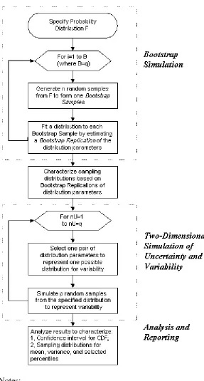
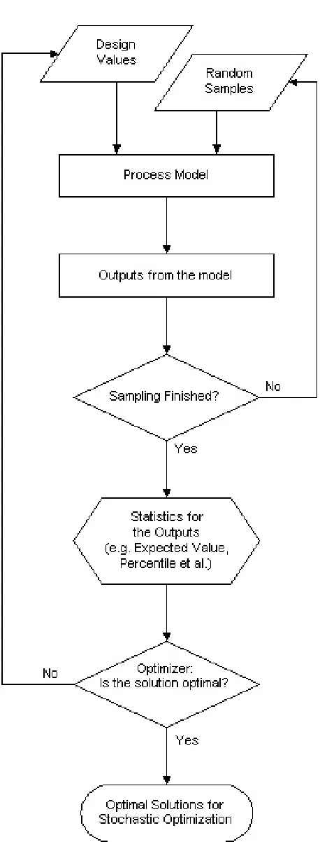
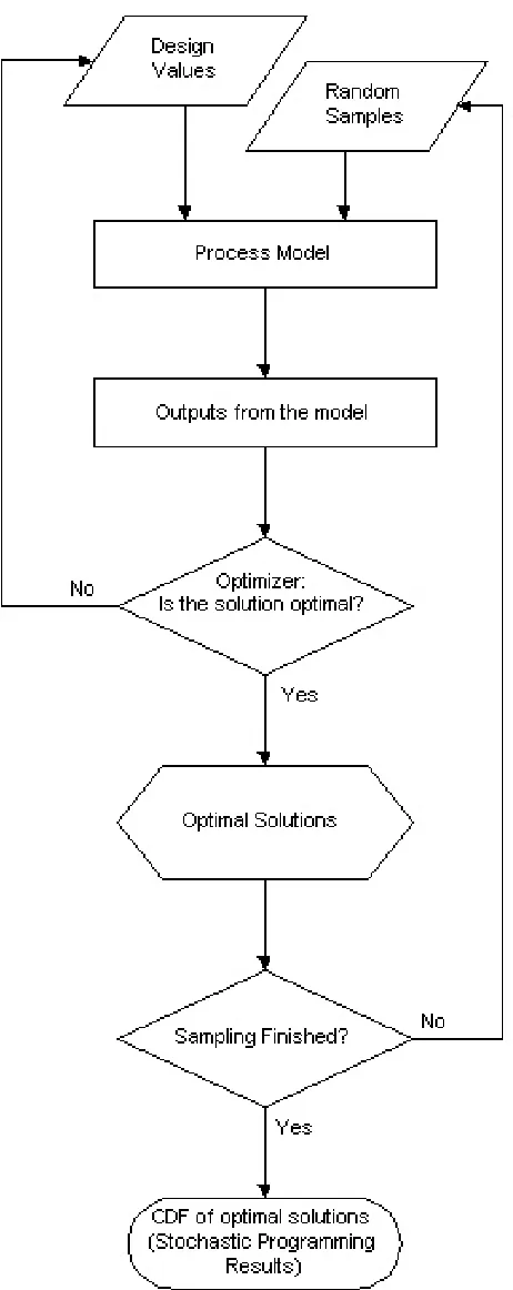
Figure 2-1. Flow Diagram for Bootstrap Simulation and Two-dimensional Simulation of Uncertainty and Variability (Frey and Rhodes, 1998)... 8 Figure 2-2. Schematic of Stochastic Optimization (adapted from Diwekar, et al., 1997).... 10 Figure 2-3. Flow Diagram of Stochastic Optimization... 11 Figure 2-4. Schematic of Stochastic Programming (adapted from Diwekar et al., 1997).... 13 Figure 2-5. Flow Diagram for Stochastic Programming ... 14 Figure 2-6. Simple Schematic for Coupled Stochastic Optimization and Programming
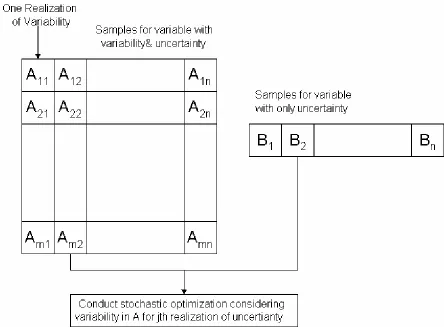
Method ... 16 Figure 2-7. Flow Diagram for Coupled Stochastic Optimization and Programming ... 17 Figure 2-8. Simple Schematic for the Two-dimensional Stochastic Programming Method 18 Figure 2-9. Flow Diagram for the Two-dimensional Stochastic Programming Method... 19 Figure 3-1. Schematic of a KRW-Gasifier based IGCC System with Hot Gas Cleanup ... 21 Figure 3-2. Fitting of Beta Distribution to Random Numbers (transformed to be between
0 and 1) from Original Triangular Distribution of CARCNV ... 29 Figure 3-3. Fitting of Beta (14.8, 14.8) Distribution to the 100 Mean Values of Bootstrap
Samples from Beta (1.0, 1.0) Distribution... 32 Figure 4-1. The General Structures of Genetic Algorithms (Gen, 1997) ... 37 Figure 4-2. Integration of Software for Optimization under Variability and Uncertainty.... 44 Figure 5-1. Optimal Expected Cost of Electricity from Stochastic Optimization
Considering Variability in Model Inputs when Expected Value of NOX
Emissions is Constrained ... 49 Figure 5-2. Sensitivity of Cost of Electricity to Gasifier Oxygen to Carbon Ratio
(RMOXG2C) when Other Design Variables are at Default Values ... 52 Figure 5-3. Sensitivity of Cost of Electricity to Gasifier Steam to Carbon Ratio
(RSTM2OX) when Other Design Variables are at Default Values... 52 Figure 5-4. Sensitivity of Cost of Electricity to Sulfur Retained in the Gasifier Bottom
Ash (XSLCNV) when Other Design Variables are at Default Values ... 52 Figure 5-5. Sensitivity of Cost of Electricity to SCR NOX Removal Efficiency (SCRAE)
when Other Design Variables are at Default Value... 53 Figure 5-6. Sensitivity of Cost of Electricity to SCR Ammonia Slip (XNH3S) when Other
Design Variables are at Default Values ... 53 Figure 5-7. Sensitivity of Cost of Electricity to Capacity Factor (CF) when Other Design
Figure 5-8. Sensitivity of Cost of Electricity to SCR Catalyst Layer Replacement Interval (REPHRS) when Other Design Variables are at Default Value ... 54 Figure 5-9. Optimal Expected Value of Cost of Electricity from Stochastic Optimization
Considering Variability in Model Inputs when 90th Percentile of NOX
Emissions is Constrained ... 55 Figure 5-10. Cumulative Probability of Optimal Cost of Electricity from Stochastic
Programming Considering Variability in Model Inputs when NOX Emissions are Constrained to Less Than or Equal to 0.2 lb/106Btu... 58 Figure 5-11. Cumulative Probability Distribution for Optimal SCR Removal Efficiency in
Stochastic Programming Considering Variability in Model Inputs when NOX Emissions are Constrained to be Less than or Equal to 0.2 lb/106Btu... 59 Figure 5-12. Dependence of Optimal SCR Removal Efficiency on the Fraction of Coal
Bound Nitrogen Converted to NH3 ... 62 Figure 5-13. Dependence of Optimal SCR Removal Efficiency on the Fraction of NH3
Converted to NOX in the gas turbine ... 62 Figure 5-14. Optimal Expected Cost of Electricity from Stochastic Optimization
Considering Uncertainty in Model Inputs when the 90th Percentile of NOX Emissions is Constrained ... 66 Figure 5-15. Cumulative Probability of Optimal Cost of Electricity from Stochastic
Programming Considering Uncertainty in Model Inputs when NOX Emissions is Constrained to be less than or equal to 0.2 lb/106Btu ... 68 Figure 5-16. Cumulative Probability of Optimal SCR Removal Efficiency from Stochastic
Programming Considering Uncertainty in Model Inputs when NOX Emissions is Constrained to be less than or equal to 0.2 lb/106Btu ... 68 Figure 5-17. Dependence of Optimal SCR Removal Efficiency on the Fraction of Coal
Bound Nitrogen Converted to NH3 ... 69 Figure 5-18. Dependence of Optimal SCR Removal Efficiency on the Fraction of NH3
Converted to NOX in Gas Turbine ... 69 Figure 5-19. NOX Emissions for Each Realization of Uncertainty under the Optimal
Designs of both Stochastic Optimization and Stochastic Programming ... 73 Figure 5-20. Cumulative Probability Distribution for Optimal Expected Cost of Electricity
from the Coupled Stochastic Optimization and Programming Method when 90th Percentile of NOX emissions ≤ 0.2 lb/106Btu ... 76 Figure 5-21. Cumulative Probability Distribution for the Optimal SCR Removal Efficiency
from the Coupled Stochastic Optimization and Programming Method when the 90th Percentile of NOX Emissions ≤ 0.2 lb/106Btu... 77 Figure 5-22. Two-dimensional Distributions for Minimum Cost of Electricity from the
Two-dimensional Stochastic Programming Method when NOX Emissions
Figure 5-23. Two-dimensional Distributions for Optimal SCR Removal Efficiency from the Two-dimensional Stochastic Programming when NOX Emissions ≤ 0.2 lb/106Btu ... 79 Figure 5-24. Cumulative Probability Distribution of Uncertainty in Expected Value of
Perfect Information with respect to Variability ... 82 Figure B-1. Cumulative Probability Distribution for Optimal Expected Cost of Electricity
from the Coupled Stochastic Optimization and Programming Method when the 90th Percentile of NOX Emissions ≤ 0.2 lb/106Btu... 114 Figure B-2. Cumulative Probability Distribution for Optimal SCR Removal Efficiency
from the Coupled Stochastic Optimization and Programming Method when the 90th Percentile of NOX Emissions ≤ 0.2 lb/106Btu... 114 Figure B-3. dimensional Distribution for the Optimal Cost of Electricity from
Two-dimensional Stochastic Programming when NOX Emissions ≤ 0.2 lb/106Btu ... 116 Figure B-4. Two-dimensional Distribution for the Optimal SCR Removal Efficiency from
Two-dimensional Stochastic Programming when NOX emissions ≤ 0.2
lb/106Btu ... 116 Figure B-5. Cumulative Probability Distribution of Expected Value of Perfect
1.0
INTRODUCTION
The emphasis of environmental design for process technologies is shifting from one pollutant to multiple pollutants, and multiple environmental media. Properly integrated system models are needed to assess the complex interactions among many components of highly coupled system. For example, Frey and Rubin (1992a) developed integrated model for environmental control in integrated gasification combined cycle systems (IGCC); Rubin
et al. (1997) developed integrated environmental control model for coal-fired power systems; Bharvirkar and Frey (1998) developed simplified performance, emissions and cost model for integrated gasification combined cycle systems (IGCC).
For all technologies in an early phase of development, there are always uncertainties in the performance and cost estimates (Frey and Rubin, 1991a). Chemical engineers and technical managers involved in research, development and demonstration (RD&D) of advanced process can benefit from a systematic approach for characterizing uncertainties in new process technologies (Frey and Rubin, 1992b). Uncertainty analysis has been applied to advanced SO2/NOX control technology (Frey and Rubin, 1991a), coal utilization and environmental control in integrated gasification combined cycle systems (Frey and Rubin, 1992; Frey, et al., 1994), integrated environmental control of coal-fired power systems (Rubin, et al., 1997). Uncertainties in model parameters were found to significantly affect the cost of the system (Frey and Rubin, 1991a; Frey and Rubin, 1992; Frey et al., 1994; Rubin et al., 1997).
optimized the SO2 control in an IGCC system. George et al. (1992) optimized the cost of electricity for an IGCC power plant, and found that annual savings for optimized design can exceed 2.2 million (mid-1990) dollars.
Combined with uncertainty analysis, optimization methods provide a powerful and rigorous tool for design of process technologies. Diwekar et al. (1997) summarized and demonstrated two methods for optimization of process models under uncertainty. One is termed as stochastic optimization, which enables one to use statistics, such as expected value, variance and other statistics, as objective function values or as constraints. Another is termed as stochastic programming, which enables one to evaluate the sensitivity of optimal solutions to uncertainty in model parameters. Stochastic optimization and programming techniques can ensure that during design phases, issues such as cost minimization, risk analysis, environmental compliance and R&D prioritization, can be fully and rigorously considered (Diwekar et al., 1997). Stochastic optimization has been applied by many researchers (Dantus and High, 1999, Hou et al., 2000; Kim and Diwekar, 2002a, 2002b). Application of stochastic programming to process models has not become popular, perhaps mostly because of its computational intensity and lack of easy-to-use software tools, although sensitivity of optimal solutions to model parameters has been studied by some researchers (Cocks et al., 1998; Jack and Tybirk, 1998; Pinto, 1998; Fournier, et al., 1999).
environmental pollutant inventory (Frey and Bammi, 2002, Frey and Zheng, 2002). Distinction between variability and uncertainty has rarely been done in probabilistic analysis or optimization of process technologies only until recently by Frey and Zhang (2003), Rooney and Biegler (2003). Rooney and Biegler consider two types of unknown input parameters, uncertainty model parameters, and variable process parameters. In the former case, a process is designed that is feasible over the entire domain of uncertain parameters, while in the later case, control variables can be adjusted during process operation to compensate for variable process parameters. However, their work does not address uncertainty in parameters that characterize variability in an input.
This thesis is organized as follows:
Chapter 2 discusses the basic concepts of variability, uncertainty, stochastic optimization and stochastic programming. Based on these, optimization techniques under both variability and uncertainty are proposed.
Chapter 3 gives an overview for the Integrated Combined Cycle System (IGCC). In this study, a KRW gasifier based IGCC system is used as an example to demonstrate optimization techniques when variability and uncertainty in model parameters are considered. Variables with variability and/or uncertainty among IGCC model parameters are identified. Probabilistic distributions are developed for these variables.
Chapter 4 describes the random number generator and optimizer used in this study. AuvTool, which was developed by Zheng and Frey (2002), is used as random number generator. Evolver, a commercial Genetic Algorithm based optimization solver, is adopted as optimizer.
Chapter 5 presents the results of optimization of the IGCC system when variability and uncertainty in model parameters are considered.
2.0
CONCEPT AND METHODOLOGY
This chapter discusses basic concepts of variability and uncertainty, stochastic optimization and stochastic programming. Based on these, coupled stochastic optimization and programming technique, and two dimensional stochastic programming are proposed. 2.1 Variability and Uncertainty
Variability is a heterogeneity of a quantity over time, space or among different members of a population (Zheng, 2002). For example, in a complex coal gasification system, many parameters are subject to variations, such as physical and chemical properties of inlet materials; material conversion rate in the system and so on. Variability can be represented by frequency distributions showing the variation of the quantity (Frey, 1997).
Uncertainty refers to a lack of knowledge regarding the true value of a quantity. Draper et al. (1987) pointed out that there are three main sources of uncertainty in any problem:
(1) Uncertainty about the structure of a model;
(2) Uncertainty about the estimates of the model parameters, assuming that the structure of the model is known;
(3) Unexplained random variation in observed variables even the structure of the model and the values of the model parameters have been known.
Distinction between variability and uncertainty can be important for policy and scientific reasons (Frey and Rhodes, 1998). In setting policy on control of emissions into environment, we may wish to protect the health of at least a given portion of the population and to do so within an acceptable confidence level. For example, we may wish to be 92% confident that we reduce the health risks of at least 96% of the population below some level. Knowledge regarding variability can be used to identify subgroup which should receive special consideration, while uncertainty can be used to prioritize additional research (Frey and Rhodes, 1998).
2.2 Sampling Technique for Variability and Uncertainty
As pointed out above, frequency distributions are used to characterize variability in a quantity, and probability distributions are used to represent uncertainty of a quantity. Numerical sampling techniques, such as Monte Carlo simulation or Latin hypercube sampling, can be employed to generate random numbers for the distributions. When variability and uncertainty in a quantity are both considered, frequency distributions are used to characterize the variability of the quantity, while there remains uncertainty regarding the frequency distribution. Two-dimensional sampling technique for uncertain frequency distributions is required to generate random numbers. In this study, the two dimensional sampling technique proposed by Frey and Rhodes (1996) is used.
parameter of interest θ, is a characteristic of the distribution F, θ = f (F), such as mean, standard deviation, or any percentile of the distribution F. An estimate of θ is the statistic θ), which is determined from the dataset, θ) = f(x). The bootstrap technique can quantify the confidence interval for θ). It involves following procedures, according to Frey and Rhodes (1998):
1. Using the data set x, the distribution F) is defined to be an estimate of the unknown population distribution F. The distribution F) can either be an empirical distribution or a parametric distribution. The former is referred to as nonparametric bootstrap, and the latter as parametric bootstrap;
2. Then, the bootstrap method repeatedly asks the question: what if the data set had been a different set of n random values from the same distribution F) ? This question is answered by repeatedly generating bootstrap samples. A bootstrap sample, x* is defined as a simulated random sample of size n taken from distribution F) . A large number, B, of independent bootstrap samples (x*1, x*2, ···, x*B) are sampled from the distribution F) . From each of the B bootstrap samples, a new statistic, θ)* is computed. Each θ)* is referred to as a bootstrap replication of θ);
3. From the B replication of θ)s, a confidence interval for θ) can be estimated.
Notes:
• B = number of bootstrap replications • q = sample size used for uncertainty • p = sample size used for variability
of variability within the population. Thus, a total of B×p random numbers are generated, representing p samples from each of B alternative frequency distributions. For each realization of uncertainty (each alternative frequency distribution), the samples are sorted to represent cumulative distribution functions. Thus there are B values for any given statistic (e.g., mean, variance, 95th percentile), which can be used to construct sampling distributions for each statistic.
2.3 Stochastic Optimization and Stochastic Programming
Optimization under uncertainty is generally divided into two categories: stochastic optimization and stochastic programming (Diwekar, et al., 1997). Stochastic optimization problems involve expected value minimization or chance constrained optimization. These problems require that some probabilistic representation of objective functions and constraints be optimized. Stochastic programming deals with the effect of uncertainty on optimal design.
2.3.1 Stochastic Optimization
A general formulation of the stochastic optimization problem can be described as (Diwekar, et al., 1997):
Objective: Min or Max Z=P1 (f(x, u))
Subject to: P2 (g(x, u)) = 0
P3 (h(x, u)) ≤ 0
Figure 2-2. Schematic of Stochastic Optimization (adapted from Diwekar, et al., 1997)
Stochastic Optimization has been applied to many problems. Watanabe and Ellis (1993) used a stochastic linear model to address an air quality management problem. Shih and Frey (1995) built a stochastic non-linear model for a coal blending problem. However, in the two works, the stochastic optimization problem was analytically transformed to an equivalent deterministic one using chance constrained programming. Therefore the approach they used only applies to certain problems. A general way is to approximate the probabilistic functions through a sampling method (Diwekar, et al., 1997). The general way involves two iterative loops: (1) the inner sampling loop and (2) the outer optimization loop. This method has been demonstrated by many researchers (Dantus and High, 1999; Hou et al., 2000; Kim and Diwekar, 2000a, 2000b). Figure 2-2 illustrates the coupling of sampling loop and optimization loop in solving a stochastic optimization problem (Diwekar et al., 1997).
variance, or 95th percentile, can be estimated. These statistics, used as objective function values or constraints, are passed to the optimizer, which either generates new design values or stops to report optimal solutions.
2.3.2 Stochastic Programming
Stochastic programming deals with the effect of uncertainty in model parameters on optimal solutions. Stochastic programming involves deterministic optimization for each random sample of uncertain variables. The formulation of stochastic programming can be represented as (Diwekar, et al., 1997):
Objective: Min or Max Z = z(x, u*)
Constraint: h (x, u*) = 0
g (x, u*) ≤ 0
Where, x = design variables,
u* = random sample for uncertain variables,
z(x, u*), h(x, u*) and g(x, u*) = functions of x and u*.
Figure 2-4. Schematic of Stochastic Programming (adapted from Diwekar et al., 1997)
probabilistic distributions of optimal solutions. A more detailed flow diagram showing procedures with regard to stochastic programming is given in Figure 2-5. Stochastic programming has been applied to an IGCC system by Diwekar et al. (1997). However, because of computational burden associated with the method, this method is rarely used. Some researchers evaluated the effect of uncertainty on optimization solutions. However their work is limited to one uncertain variable at a time (Fournier et al., 1999; Pinto, 1998), or to a very small number of simulations (Bak and Tybirk, 1998; Cocks et al., 1998).
2.4 Optimization Considering both Variability and Uncertainty
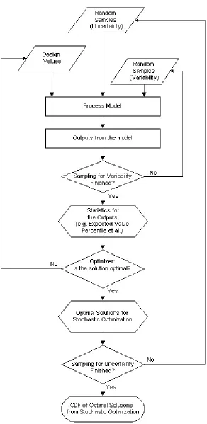
The coupled stochastic optimization and programming technique involves stochastic optimization for each alternative frequency distribution which represents variability. During each stochastic optimization, a point estimate result for each alternative frequency distribution of model results is optimized. The output of this method is a probability distribution of optimal solutions from stochastic optimization. This method can be used to assess the effect of uncertainty on stochastic optimization results.
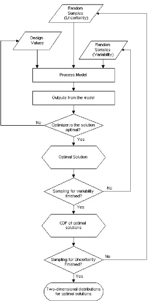
Two-dimensional stochastic programming involves deterministic optimization for each sample of variability and uncertainty. The output of this method will be a two dimensional distribution for deterministic optimal solutions. This method enables one to evaluate the effect of both variability and uncertainty on optimal solutions.
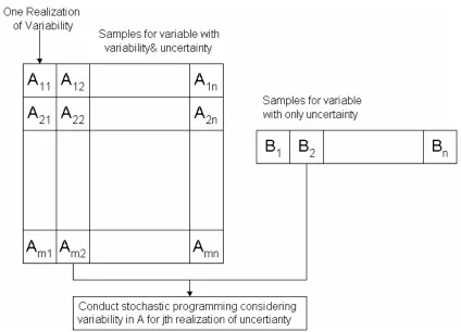
The two methods are illustrated by an example in which one variable P among model parameters is assumed to be variable and uncertain and another variable Q among model parameters is assumed to be uncertain.
Let Aij (1 ≤ i ≤ m and 1 ≤ j ≤ n) represents random numbers generated from the two- dimensional sampling technique for the variable P, where m is the realization number for variability and n is the realization number for uncertainty. Let Bj (1 ≤ j ≤ n) represents the random numbers generated from Monte Carlo simulation for the variable Q, where n is the realization number for uncertainty.
The algorithm for coupled stochastic optimization and programming method is described as follows:
1. j=0;
2. j = j+1, conduct stochastic optimization for Aij ( i from 1 to m) and Bj. Aij ( i
is the jth random sample of Q; 3. If j <n, then go back to step 2; If j =n, then stop.
The results are n optimal solutions from stochastic optimization, which can be used to construct a cumulative probability distribution. Figure 2-6 shows a simple schematic of the method. For each realization of uncertainty in variables with both variability and uncertainty, stochastic optimization is done. A detailed flow diagram is given in Figure 2-7.
The algorithm for the two-dimensional stochastic programming technique is described below:
1. j=0;
2. j = j +1 and i=0;
3. i = i +1; for Aij and Bj, conduct deterministic optimization and find the optimal solution;
4. if i<m then go back to step 3, otherwise go forward to step 5; 5. if j<n then go back to step 2, otherwise stop.
The results are m×n deterministic optimization solutions. Step 3 and step 4 constitute a stochastic programming procedure. Figure 2-8 shows the simple schematic of the method. Detailed flow diagram is given in Figure 2-9.
3.0
OVERVIEW OF INTEGRATED GASIFICATION COMBINED
CYCLE (IGCC) SYSTEM
Environmental regulations are one of the factors that spur the development of new coal-based electric power generation technologies. Conventional emission control systems for a new pulverized coal-fired power plant typically consist of a wet limestone flue gas desulfurization (FGD) system for SO2 control, an electrostatic precipitator (ESP) for PM removal, and combustion control for NOX reduction. Selective Catalytic Reduction (SCR) is a post-combustion NOX control technology that has been demonstrated in Japan, German and a small number of U.S. coal-fired power plants and is expected to be required to comply with the New Source Performance Standard (NSPS) (EPA, 1997). With the stringency of the current NSPS, few new coal plants are currently being built in the U.S.
Integrated Gasification Combined Cycle (IGCC) system is an alternative to the conventional pulverized coal (PC) combustion system. In a combined cycle plant, fuel is burned in a gas turbine, and the hot exhaust gas is used to generate steam for a steam cycle. Electric generators on both the gas turbine and steam turbine generate electricity. IGCC systems are capable of NOX emissions comparable to or less than those of PC plants equipped with SCR, as well as high levels of SO2 control (EPRI, 1988). Meanwhile, IGCC systems offer other advantages such as phased construction, fuel flexibility, reduced solid waste, a modular design and a capability to produce useful co-products. The U.S Department of Energy is pursuing development of a new generation of gasification systems intended to offer an environmentally and economically viable alternative for power generation in the U.S. (U.S. DOE, 2000).
Figure 3-1. Schematic of a KRW-Gasifier based IGCC System with Hot Gas Cleanup
of the coal is combusted to release heat, while the remainder participates in endothermic gasification reactions with steam to produce a syngas containing CO and H2. The syngas that exits from the gasifier enters a high temperature gas cooling unit, where it is quenched by water. Subsequently it is cleaned of impurities such as particulate matter and sulfur compounds, in the gas cleanup unit.
The clean fuel gas is sent to a gas turbine, where recovered energy is used to rotate generator for electricity. The hot exhaust gas from the gas turbine passes through a Heat Recovery Steam Generator (HRSG). In the HRSG, the syngas is cooled and the transferred heat is used to generate hot boiler feed water, saturated steam, and superheated steam. Superheated steam is used to produce electric power via a steam turbine. Post combustion air pollution control technologies, such as Selective Catalytic Reduction (SCR) for NOX control, can be located within the HRSG (Frey et al., 1994).
fluidized bed (Frey and Rubin, 1990). The KRW-based IGCC systems include a hot gas cleanup system featuring in-bed desulfurization in the gasifier with limestone or dolomite, subsequent sulfur removal from the fuel gas with a zinc ferrite sorbent, a high efficiency cyclone and ceramic filters for particulate removal, sulfation of spent limestone and conversion of carbon remaining in the ash by using a circulating bed boiler (Frey and Rubin, 1992; Frey et al., 1994; Bharvirkar and Frey, 1998).
3.1 Performance, Emissions and Cost Model for KRW Gasifier-based IGCC System A simplified performance, emissions and cost model of a KRW gasifier-based IGCC system developed by Bharvirkar and Frey (1998) is used in this study. The performance and emissions part of this model is a regression model based on probabilistic analysis of a detailed ASPEN-based model. The accuracy of the simplified model is typically within a percent compared with the ASPEN model (Bharvirkar and Frey, 1998). It provides a selection of four process configurations featuring two gas turbine designs and the inclusion or exclusion of SCR for NOX control. A description of the four configurations is given in Table 3-1.
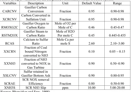
In the model, there are 10 independent variables that can be specified by the user, which are shown in Table 3-2. Based on these 10 independent variables, the performance model calculates values for about 60 dependent variables, which are served later as input values to the cost model.
Table 3-1. Description of Configurations Considered in the Model
Case Gas Turbine
Pressure Ratio
Gas Turbine Inlet Temperature (°K)
Selective Catalytic Reduction 1 2 3 4 15.0 15.0 13.5 13.5 2350 2350 2300 2300 No Yes Yes No Table 3-2. Input Variables for the Simplified Performance Model of IGCC System
Variables Description Unit Default Value Range
CARCNV
Gasifier Carbon
Conversion Fraction 0.95 0.90-0.98
XCRCNV Carbon Converted in Sulfation Unit Fraction 0.95 0.90-0.98 RMOXG2C Gasifier Oxygen to Carbon Ratio Mole of O2 per Mole of C 0.46 0.45-0.47
RSTM2OX Gasifier Steam to Carbon Ratio
Mole of H2O
Per mole C 0.45 0.445-0.455
RCAS
Calcium to Sulfur Ratio
Mole Ca per
mole S 2.60 2.10~3.00
XXCRN
Fraction of Coal bound Nitrogen
converted to NH3 Fraction 0.10 0.05 ~ 0.15 XXNH3
Fraction of NH3 converted to NOX in
Gas Turbine Fraction 0.90 0.50~0.90
XSLCNV
Sulfur retained in
Gasifier Bottom Ash Fraction 0.90 0.80-0.95 SCRAE
SCR NOX removal
Efficiency Fraction 0.80 0.50-0.90
XNH3S SCR NH3 Slip ppm 10.00 5.00-20.00
(Source: Bharvirkar and Frey, 1998)
work, we adopted this relationship, which is shown in equation 3-1.
− − − = XSLCNV b XSLCNV a RCAS 1 1 ) exp( (3-1)
Where, RCAS = calcium to sulfur ratio (mole calcium per mole of sulfur); XSLCNV = sulfur retained in gasifier bottom ash (fraction); a=0.233;
The cost model was developed and updated by Frey and Rubin (Frey and Rubin, 1990; Frey et al., 1994, Frey, 1994). The cost model calculates capital cost, annual fixed operating cost and variable operating cost for 11 process areas, which are coal handling, boiler feed water systems, limestone handling, gas turbine, oxidant feed, heat recovery steam generation, gasification, selective catalytic reduction, zinc ferrite process, steam turbine, sulfation and general facilities.
By default, the original cost model reports cost on the basis of January, 1989. In this work, the model is modified to report the cost on the basis of January, 2002, by using chemical engineering plant cost index (CI) and industrial chemicals producer price index (CICPPI) for January, 2002, which are 390.3 and 417.95, respectively (Chemical Week Publish, 2002). These values are not substantially different from those of January, 1989. CI for January of 2002 is only 10% higher than that of January, 1989 which is 354.7. CICPPI for January of 2002 is 6.6% higher than that of January, 1989 which is 391.87.
3.2 Interface of the Model
3.3 Variability and Uncertainty in Model Inputs
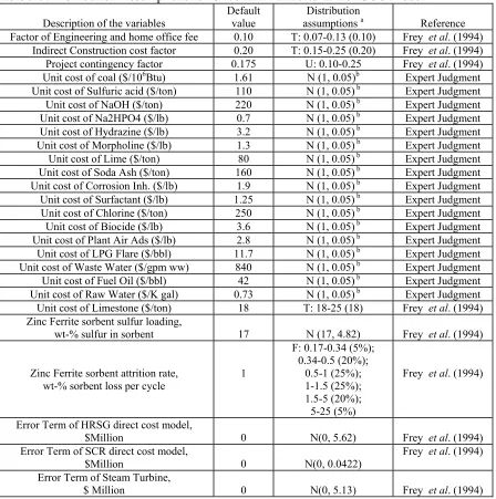
For the IGCC model discussed above, 27 variables were identified as uncertain variables. For each uncertain variable, probabilistic distribution is used to characterize its uncertainty. The selection of these variables and development of uncertainty assumptions are mainly based on the work by Frey et al. (1994). They identified and estimated uncertainties for these parameters based on literature review, data analysis, and elicitation of expert judgments from engineers involved in IGCC technology development at DOE’s Morgantown Energy Technology Center (DOE/METC) (Frey et al., 1994). Table 3-3 summarizes the distribution assumptions for the uncertain variables.
Table 3-3. Distribution Assumptions for Uncertain Variables in the IGCC Model Description of the variables
Default value
Distribution
assumptions a Reference
Factor of Engineering and home office fee 0.10 T: 0.07-0.13 (0.10) Frey et al. (1994) Indirect Construction cost factor 0.20 T: 0.15-0.25 (0.20) Frey et al. (1994) Project contingency factor 0.175 U: 0.10-0.25 Frey et al. (1994) Unit cost of coal ($/106Btu) 1.61 N (1, 0.05)b Expert Judgment
Unit cost of Sulfuric acid ($/ton) 110 N (1, 0.05) b Expert Judgment
Unit cost of NaOH ($/ton) 220 N (1, 0.05) b Expert Judgment
Unit cost of Na2HPO4 ($/lb) 0.7 N (1, 0.05) b Expert Judgment
Unit cost of Hydrazine ($/lb) 3.2 N (1, 0.05) b Expert Judgment
Unit cost of Morpholine ($/lb) 1.3 N (1, 0.05) b Expert Judgment
Unit cost of Lime ($/ton) 80 N (1, 0.05) b Expert Judgment
Unit cost of Soda Ash ($/ton) 160 N (1, 0.05) b Expert Judgment
Unit cost of Corrosion Inh. ($/lb) 1.9 N (1, 0.05) b Expert Judgment
Unit cost of Surfactant ($/lb) 1.25 N (1, 0.05) b Expert Judgment
Unit cost of Chlorine ($/ton) 250 N (1, 0.05) b Expert Judgment
Unit cost of Biocide ($/lb) 3.6 N (1, 0.05) b Expert Judgment
Unit cost of Plant Air Ads ($/lb) 2.8 N (1, 0.05) b Expert Judgment
Unit cost of LPG Flare ($/bbl) 11.7 N (1, 0.05) b Expert Judgment
Unit cost of Waste Water ($/gpm ww) 840 N (1, 0.05) b Expert Judgment
Unit cost of Fuel Oil ($/bbl) 42 N (1, 0.05) b Expert Judgment
Unit cost of Raw Water ($/K gal) 0.73 N (1, 0.05) b Expert Judgment
Unit cost of Limestone ($/ton) 18 T: 18-25 (18) Frey et al. (1994) Zinc Ferrite sorbent sulfur loading,
wt-% sulfur in sorbent 17 N (17, 4.82) Frey et al. (1994)
Zinc Ferrite sorbent attrition rate,
wt-% sorbent loss per cycle 1
F: 0.17-0.34 (5%); 0.34-0.5 (20%);
0.5-1 (25%); 1-1.5 (25%); 1.5-5 (20%); 5-25 (5%)
Frey et al. (1994)
Error Term of HRSG direct cost model,
$Million 0 N(0, 5.62) Frey et al. (1994) Error Term of SCR direct cost model,
$Million 0 N(0, 0.0422) Frey et al. (1994) Error Term of Steam Turbine,
$ Million 0 N(0, 5.13) Frey et al. (1994)
a: T=Triangular distribution, lower bound and upper bound are given, mode is in parenthesis;
U=Uniform distribution, lower and upper bound are given;
N=Normal distribution, mean value and standard deviation are given;
F=Fractile distribution, lower and upper bound of each range are given, along with the possibility of samples within that range;
b: on a relative basis, which means random samples from the distribution should be multiplied with default
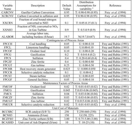
Table 3-4: Distribution Assumptions for the Variables with both Variability and Uncertainty in the IGCC Model
Variable
Name Description Default Value
Distribution Assumptions for
variability a Reference
CARCNV Gasifier Carbon Conversion 0.95 T: 0.90-0.98 (0.95) Frey et al. (1994) XCRCNV Carbon Converted in sulfation unit 0.95 T:0.90-0.98 (0.95) Frey et al. (1994) XXCRN Fraction of coal bound nitrogen converted to NH3 0.1 T: 0.05-0.15 (0.1) Frey et al. (1994) XXNH3 Fraction of NHin Gas Turbine 3 converted to NOX 0.9 T: 0.5-0.9 (0.9) Frey et al. (1994) ALABOR including burdens ($/hour) Average labor rate, 19.7 N(19.7,0.647) Frey et al. (1994)
Contingencies of Process Areas
FPCCH Coal handling 0.05 U: 0.00-0.10 Frey and Rubin (1991) FPCL Limestone handling 0.05 U:0.00-0.10 Frey and Rubin (1991) FPCOF Oxidant feed 0.10 U: 0.00-0.20 Frey and Rubin (1991) FPCG Gasification 0.2 T: 0.0-0.4 (0.2) Frey and Rubin (1991) FPCS Sulfation 0.4 T: 0.20-0.60 (0.4) Frey and Rubin (1991) FPCZF Zinc ferrite 0.4 U: 0.00-0.80 Frey and Rubin (1991) FPCGT Gas turbine 0.25 U: 0.00-0.50 Frey and Rubin (1991) FPCHR Heat recovery steam generator 0.025 U: 0.000-0.050 Frey and Rubin (1991) FPCCR Selective catalytic reduction 0.1 U: 0.00-0.2 Frey and Rubin (1991) FPCST Steam turbine 0.025 U: 0.00-0.05 Frey and Rubin (1991) FPCGF General facilities 0.05 U: 0.00-0.10 Frey and Rubin (1991)
Maintenance Factors of Process Areas
FMCOF Oxidant feed 0.02 T: 0.01-0.03 (0.02) Frey and Rubin (1991) FMCG Gasification 0.045 T:0.03-0.06 (0.045) Frey and Rubin (1991) FMCS Sulfation 0.04 T: 0.03-0.06 (0.04) Frey and Rubin (1991) FMCZF Zinc ferrite 0.03 T: 0.03-0.06 (0.03) Frey and Rubin (1991) FMCGT Gas turbine 0.02 T:0.015-0.06 (0.02) Frey and Rubin (1991) FMCCR Selective catalytic reduction 0.02 T: 0.01-0.03 (0.02) Frey et al. (1994)
Unit Cost of Materials
BCCSRC SCR catalyst ($/ft^3) 250 T:250-660 (350) Frey et al. (1994) BCNH3 Ammonia ($/ton) 150 U(150, 225) Frey et al. (1994) BCZFSO Zinc Ferrite sorbent ($/lb) 3.00 T: 0.75-5.00 (3.00) Frey et al. (1994) BCASHD Unit cost of Ash Disposal ($/ton) 10 T: 10-25 (10) Frey et al. (1994)
a: T=Triangular distribution, lower bound and upper bound are given, mode is in parenthesis;
U=Uniform distribution, lower and upper bound are given;
N=Normal distribution, mean value and standard deviation are given;
higher than 0.98, which causes the IGCC model not to work correctly. To resolve this problem, distributions in Table 3-4 are transformed to beta distribution. For example, variable X is constrained by a lower bound of a and an upper bound of b. X is first transformed to X′ by Equation (3-2). Thus, X′ is bounded by 0 and 1. Variability in X′ is represented by a beta distribution. When bootstrap samples are generated for X′, X can be calculated from X′ by Equation (3-3). Since bootstrap samples for beta distribution are strictly bounded by 0 and 1, samples for X are strictly bounded within a and b.
) /( ) (
' X a b a
X = − − (3-2) '
) (b a X a
X = + − × (3-3)
Fitting a Distribution for CARCNV
Data (n=100)
Beta
C
u
m
u
lat
iv
e
P
ro
b
ab
ili
ty
0.0 0.2 0.4 0.6 0.8 1.0
0.0 0.2 0.4 0.6 0.8 1.0
Figure 3-2. Fitting of Beta Distribution to Random Numbers (transformed to be between 0 and 1) from Original Triangular Distribution of CARCNV
Figure 3-2 shows the fitted beta(2.5, 2.1) distribution compared to the transformed random samples. The beta(2.5, 2.1) distribution fits the random samples very well. The KS Test was used to determine whether the fit is good. In this case, the K-S statistics is 0.031, which is lower than the critical value of 0.088, thus indicating a good fit.
Table 3-5 summarizes the transformed distributions for variables with variability. For each variable, beta distributions were found to approximate the original distribution assumptions very well. Table 3-6 summarizes K-S testing results for each variable. Each fitting passes the K-S test, indicating good fit. The transformed distributions, not the original distributions shown in Table 3-4, are used in this study.
Table 3-5. Distribution Assumptions for the Variables with both Variability and Uncertainty in the IGCC Model
Variable
Name Description
Original Distribution for
variability a Transformed Distribution for variability b
CARCNV Gasifier Carbon Conversion T: 0.90-0.98 (0.95) 0.90 + 0.08* Beta (2.6, 2.2) XCRCNV Carbon Converted in sulfation unit T:0.90-0.98 (0.95) 0.90 + 0.08*Beta (2.6, 2.2)
XXCRN
Fraction of coal bound nitrogen
converted to NH3 T: 0.05-0.15 (0.1) 0.05 + 0.10*Beta (2.5, 2.5) XXNH3
Fraction of NH3 converted to NOX
in Gas Turbine T: 0.5-0.9 (0.9) 0.5 + 0.4*Beta (2.0, 1.0) ALABOR including burdens ($/hour) Average labor rate, N(19.7,0.647) Normal (19.7, 0.649)
Contingencies of Process Areas
FPCCH coal handling U: 0.00-0.10 0.10* Beta(1,1) FPCL limestone handling U:0.00-0.10 0.10* Beta(1,1)
FPCOF oxidant feed U: 0.00-0.20 0.20* Beta(1,1)
FPCG gasification T: 0.0-0.4 (0.2) 0.20* Beta(2.5,2.5) FPCS sulfation T: 0.20-0.60 (0.4) 0.20+ 0.40* Beta(2.5,2.5)
FPCZF zinc ferrite U: 0.00-0.80 0.80* Beta(1,1)
FPCGT gas turbine U: 0.00-0.50 0.50* Beta(1,1)
FPCHR heat recovery steam generator U: 0.000-0.050 0.050* Beta(1,1) FPCCR selective catalytic reduction U: 0.00-0.2 0.20* Beta(1,1) FPCST steam turbine U: 0.00-0.05 0.05* Beta(1,1) FPCGF general facilities U: 0.00-0.10 0.10* Beta(1,1)
Maintenance Factors of Process Areas
FMCOF oxidant feed T: 0.01-0.03 (0.02) 0.01+0.02* Beta(2.5,2.5) FMCG gasification T: 0.03-0.06 (0.045) 0.03+0.03* Beta(2.5,2.5) FMCS sulfation T: 0.03-0.06 (0.04) 0.03+0.03* Beta(2.1, 2.6) FMCZF zinc ferrite T: 0.03-0.06 (0.03) 0.03+0.03* Beta(1.0,2.0) FMCGT gas turbine T: 0.015-0.06 (0.02) 0.015+0.045* Beta(1.3, 2.3) FMCCR selective catalytic reduction T: 0.01-0.03 (0.02) 0.01+0.02* Beta(2.5,2.5)
Unit Cost of Materials
BCCSRC SCR catalyst ($/ft^3) T:250-660 (350) 250+410* Beta(1.6, 2.1) BCNH3 Ammonia ($/ton) U(150, 225) 150+75* Beta(1,1) BCZFSO Zinc Ferrite Sorbent ($/lb) T: 0.75-5.00 (3.00) 0.75+4.25* Beta (2.5, 2.3) BCASHD Unit cost of Ash Disposal ($/ton) T: 10-25 (10) 10 +15* Beta (1.0, 2.0)
a: T=Triangular distribution, lower bound and upper bound are given, mode is in parenthesis;
U=Uniform distribution, lower and upper bound are given.
b: Normal = Normal distribution, mean value and standard deviation are given in parenthesis;
Table 3-6. K-S Test Results of Beta Distributions fitted to Transformed Random Samples from Original Distributions of Variability
Variable Name
Original Distribution a
Original distribution transformed to within 0 and 1 a
Fitted Beta
distribution a K-S Test b Test K-S
pass/failed? c
CARCNV
T: 0.90-0.98
(0.95) T: 0-1 (0.625) Beta (2.6, 2.2) 0.031 Passed XCRCNV T:0.90-0.98 (0.95) T: 0-1 (0.625) Beta (2.6, 2.2) 0.030 Passed XXCRN T: 0.05-0.1(0.1) T: 0-1 (0.5) Beta (2.5, 2.5) 0.023 Passed XXNH3 T: 0.5-0.9 (0.9) T: 0-1 (1) Beta (2.0, 1.0) 0.013 Passed FPCCH U: 0.00-0.10 U: 0-1 Beta(1,1) 0.012 Passed
FPCL U:0.00-0.10 U: 0-1 Beta(1,1) 0.012 Passed
FPCOF U: 0.00-0.20 U: 0-1 Beta(1,1) 0.013 Passed FPCG T: 0.0-0.4 (0.2) T: 0-1 (0.5) Beta(2.5,2.5) 0.025 Passed FPCS T: 0.20-0.60 (0.4) T: 0-1 (0.5) Beta(2.5,2.5) 0.026 Passed FPCZF U: 0.00-0.80 U: 0-1 Beta(1,1) 0.012 Passed FPCGT U: 0.00-0.50 U: 0-1 Beta(1,1) 0.012 Passed FPCHR U: 0.000-0.050 U: 0-1 Beta(1,1) 0.012 Passed FPCCR U: 0.00-0.2 U: 0-1 Beta(1,1) 0.013 Passed FPCST U: 0.00-0.05 U: 0-1 Beta(1,1) 0.012 Passed FPCGF U: 0.00-0.10 U: 0-1 Beta(1,1) 0.013 Passed FMCOF T: 0.01-0.03 (0.02) T: 0-1 (0.5) Beta(2.5,2.5) 0.025 Passed FMCG T: 0.03-0.06 (0.045) T: 0-1 (0.5) Beta(2.5,2.5) 0.025 Passed FMCS
T: 0.03-0.06
(0.04) T: 0-1 (0.333) Beta(2.1, 2.6) 0.032 Passed FMCZF T: 0.03-0.06 (0.03) T: 0-1 (0) Beta(1.0,2.0) 0.012 Passed FMCGT T: 0.015-0.06 (0.02) T: 0-1 (0.11) Beta(1.3, 2.3) 0.039 Passed FMCCR T: 0.01-0.03 (0.02) T: 0-1 (0.5) Beta(2.5,2.5) 0.024 Passed BCSCRC
T:250-660
(350) T:0-1 (0.244) Beta(1.6, 2.1) 0.046 Passed
BCNH3 U(150, 225) U:0-1 Beta(1,1) 0.012 Passed
BCZFSO T: 0.75-5.00 (3.00) T: 0-1 (0.53) Beta (2.5, 2.3) 0.027 Passed BCASHD T: 10-25 (10) T:0-1 (0) Beta (1.0, 2.0) 0.012 Passed
a: T=Triangular distribution, lower bound and upper bound are given, mode is in parenthesis
U=Uniform distribution, lower and upper bound are given; Beta = Beta distribution, shape parameters are given in parenthesis.
b: Kolmogorov-Smirnov Test of beta distribution to transformed random samples (according to Equation 3-2) from original distributions.
Figure 3-3. Fitting of Beta (14.8, 14.8) Distribution to the 100 Mean Values of Bootstrap Samples from Beta (1.0, 1.0) Distribution
Table 3-7. Distribution Assumptions for Uncertainties in the Mean Value of the Variables with both Variability and Uncertainty in the IGCC Model
Variable
Name Description Distribution Assumptions a K-S Test b Passed/Failed K-S Test c
CARCNV Carbon Conversion Gasifier 0.90 + 0.08* Beta (30, 25) 0.044 Passed XCRCNV Carbon Converted in sulfation unit 0.90 + 0.08* Beta (27, 22) 0.042 Passed
XXCRN
Fraction of coal bound nitrogen
converted to NH3 0.05 + 0.10* Beta (30, 30) 0.039 Passed XXNH3 converted to NOFraction of NH3X
in Gas Turbine 0.5 + 0.4* Beta (37, 17) 0.047 Passed ALABOR Average labor rate, including burdens
($/hour)
Normal (19.7, 0.065) 0.053 Passed Contingencies of Process Areas
FPCCH Coal handling 0.10* Beta (14.8,14.8) 0.049 Passed FPCL Limestone handling 0.10* Beta (14.8,14.8) 0.049 Passed FPCOF Oxidant feed 0.20* Beta (14.8,14.8) 0.049 Passed
FPCG Gasification 0.20* Beta (29.5,29.5) 0.039 Passed FPCS Sulfation 0.20+ 0.40* Beta (29.5,29.5) 0.039 Passed
FPCZF Zinc ferrite 0.80* Beta (14.8,14.8) 0.049 Passed FPCGT Gas turbine 0.50* Beta (14.8,14.8) 0.049 Passed FPCHR steam generator Heat recovery 0.050* Beta (14.8,14.8) 0.049 Passed FPCCR catalytic reduction Selective 0.20* Beta (14.8,14.8) 0.049 Passed FPCST Steam turbine 0.05* Beta (14.8,14.8) 0.049 Passed FPCGF General facilities 0.10* Beta (14.8,14.8) 0.049 Passed
Maintenance Factors of Process Areas
FMCOF Oxidant feed 0.01+0.02* Beta (30,30) 0.039 Passed FMCG Gasification 0.03+0.03* Beta (30,30) 0.039 Passed FMCS Sulfation 0.03+0.03* Beta (23, 30) 0.051 Passed FMCZF Zinc ferrite 0.03+0.03* Beta (30,43) 0.058 Passed FMCGT Gas turbine 0.015+0.045* Beta (13, 22) 0.047 Passed FMCCR catalytic reduction Selective 0.01+0.02* Beta (29.5,29.5) 0.039 Passed
Unit Cost of Materials
BCCSRC SCR catalyst ($/ft^3) 250+410* Beta (1.8, 2.5) 0.060 Passed BCNH3 Ammonia ($/ton) 150+75* Beta (14.8,14.8) 0.039 Passed BCZFSO Zinc Ferrite Sorbent ($/lb) 0.75+4.25* Beta (32,32) 0.048 Passed BCASHD
Unit cost of
Ash Disposal ($/ton) 10 +15* Beta (10, 20) 0.037 Passed
a: Beta = Beta distribution, shape parameters are given in parenthesis.
b: Kolmogorov-Smirnov Test of beta distribution to mean values of bootstrap samples of each variable.
4.0
SOFTWARE IMPLEMENTATION
This chapter discusses the software implementation for doing optimization under variability and/or uncertainty. Optimization of process models under variability and/or uncertainty includes three parts: random number generator, optimization solver, and the process model. The process model used in this study is a simplified performance, emissions and cost model for a KRW gasifier based IGCC system, and has been introduced in Chapter 3. In this Chapter, the random number generator, optimization solver, and how the three parts are integrated into a single framework are discussed.
4.1 Random Number Generator
In this study, random numbers for variability, uncertainty, or both variability and uncertainty in parameters are generated through an existing software ―AuvTool (Analysis of Uncertainty and Variability Tool). AuvTool was developed by Zheng and Frey (2002). It uses a two-dimensional sampling method featuring bootstrap simulation for simultaneously simulating variability and uncertainty. This technique was proposed by Frey and Rhodes (1996), and has been discussed in Chapter 2. AuvTool can also generate one-dimensional samples representing only variability or uncertainty based on Monte Carlo simulation. AuvTool uses combined Multiple Recursive Generators (MRGs) presented by L’Ecuyer (1996) as a pseudo-random number generator (Frey et al., 2002). Random numbers generated from AuvTool are saved as a Microsoft Excel file. Through this file, random samples are read and used in the optimization process.
4.2 Overview of the Optimizer
4.2.1 Overview of Genetic Algorithms
Genetic algorithm (GA) is a powerful stochastic search and optimization technique based on principles from evolution theory. Holland (1975) pioneered the development of GA. In recent years, GA has been widely applied to many fields, such as air quality management (Loughlin et al., 2000), chemical processes or equipment design (Wang et al., 1996; Tayal et al. 1999), and water resource management (Wardlaw and Sharif, 1999; Burn and Yulianti, 2001).
formed. With each generation, the average fitness of individuals will be improved. This process of crossover, mutation and selection is repeated until some stopping criteria are met, such as computational time, number of generations and so on. Let P(t) and C(t) be parents and offspring (children) in the current generation t. The procedures in genetic algorithm can be described as follows (Gen, 1997):
Begin: t=0
Initialize P (t);
Evaluate P (t);
While (not termination condition) do
Recombine P (t) to yield C (t);
(Recombination includes crossover and mutation)
Evaluate C (t);
Select P (t+1) from P (t) and C (t);
t = t +1;
End
End
Figure 4-1. The General Structures of Genetic Algorithms (Gen, 1997)
4.2.2 Overview of Evolver
Evolver is a genetic algorithm (GA) based optimization solver developed by Palisade Corporation (Palisade, 1998). It is built as a Microsoft Excel Add-in. The basic steps required to run Evolver are summarized as follows:
(1) Set the objective value for the problems;
(2) Select design variables and setting constraint on design variables;
(3) Specify crossover and mutation operators and rates. Besides the default crossover and mutation operator, Evolver also provides several other operators, such as linear operator and boundary mutations, which can improve the performance and efficiency for certain problems. The default crossover and mutation operator are used
throughout the study. The linear operator is also used since there are many linear equations in the IGCC model (Nonlinear equations also exist in the IGCC model). As pointed out in the user’s guide of Evolver, the linear operator is designed to solve the problem where optimal solutions lies on the boundary of the search space and is particularly suited for solving linear optimization problem (Palisade, 1998). The default crossover and mutation rates are 0.5 and 0.1, respectively, in Evolver, and users have the option to change them. In this study, the default value for crossover and mutation rate is used.
(4) Set other constraints;
(6) Choose stopping conditions, such as number of trials, running minutes, or change of objective value after a certain number of valid trials is less than some percentage. The last one is the most popular stopping condition (Palisade, 1998). In this study, we use change of objective value after 200 valid trials of less than 1% as stopping condition, which is more conservative than the default value of Evolver (change of objective value after 100 valid trials is less than 1%);
After setting these conditions, one can set the Evolver to start optimizing. When the stopping criteria is met, Evolver stops the optimization process, and reports the best objective function value, and optimal design variables at which the best objective function value is achieved.
4.2.3 Performance of GA in Optimization of Process Models
Before doing optimization under variability and/or uncertainty, two less computationally intensive deterministic optimization cases were carried out to evaluate the performance of Evolver for optimization of process models. The first one involves optimal control of NOX emissions in an IGCC system, and the second one involves optimal control of SO2 emissions in an IGCC system.
Case 1: Optimal Control of NOX Emissions in an IGCC System
The IGCC system in this case features a gas turbine design with an inlet temperature of 2350 K, pressure ratio of 13.5, and a Selective Catalytic Reduction (SCR) for post-combustion NOX control. This system corresponds to configuration 2 in the performance and cost model discussed in Chapter 3.
The objective of this problem is to minimize of cost of electricity in mills/kWh, when NOX emissions are constrained to be less than or equal to 0.3 lb/106Btu. It is a nonlinear programming problem, since there are both linear and nonlinear equations in the IGCC model. Design variables are gasifier carbon conversion (CARCNV), gasifier oxygen to carbon ratio (RMOXG2C), gasifier steam to carbon ratio (RSTM2OX), sulfur retained in gasifier bottom ash (XSLCNV), SCR NOX removal efficiency (SCRAE) and SCR NH3 slip (XNH3S). Description of the optimization problem is summarized in Table 4-1.
The optimal solutions from Evolver and SQP are summarized in Table 4-2. The optimal cost of electricity is 51.43 mills/kWh found by Evolver, and 51.42 mills/kWh by SQP. The optimal design variable values from the two methods are very close. The optimal points are also similar as shown in Table 4-2. There is a difference regarding the optimal ammonia slip from the two methods. This implies that ammonia slip does not substantially affect the cost of electricity.
Table 4-1. Deterministic Optimization of NOX Emissions Control in an IGCC System Objective Minimization of Cost of Electricity (mills/kWh) Constraint NOX emissions ≤ 0.3 lb/106Btu
Design variables Gasifier Carbon Conversion (CARCNV) Gasifier Oxygen to Carbon Ratio (RMOXG2C)
Gasifier Steam to Carbon Ratio (RSTM2OX) Sulfur retained in Gasifier bottom ash (XSLCNV)
SCR NOX removal efficiency (SCRAE) SCR NH3 slip (XNH3S)
Constraint on design values 0.90 ≤ CARCNV ≤ 0.98 0.45 ≤ RMOXG2C ≤ 0.47 0.445 ≤ RSTM2OX ≤ 0.455
0.80 ≤ XSLCNV ≤ 0.95 0.50 ≤ SCRAE ≤ 0.90
5.0 ≤ XNH3S ≤ 20.0
Table 4-2. Summary of Optimal Solutions from Evolver and SQP for NOX Emission Control in an IGCC System
Evolver IMSL
Optimization method
Genetic Algorithm (GA)
Successive Quadratic Programming (SQP) Optimal cost of electricity
(year 1989 mills/kWh) 51.43 51.42
Constraint value
at optimal point (lb/106 Btu) 0.3000 0.3000
Optimal design values
CARCNV=0.980 RMOXG2C=0.450 RSTM2OX=0.455 XSLCNV=0.945 SCRAE=0.517 XNH3S=5 CARCNV=0.980, RMOXG2C=0.450 RSTM2OX=0.455 XSLCNV=0.944 SCRAE=0.515 XNH3S=9.935
Case 2: Optimization of SO2 Emission Control in an IGCC System
In this case, the SO2 emissions control in the IGCC system is optimized with Evolver. Results from Evolver are compared with published data. The objective of this case study is to see whether or not optimal solutions can be comparable to those from other researchers.
Three design variables are chosen, which are in-bed desulfurization efficiency, zinc ferrite absorption cycle time and maximum vessel height to diameter ratio (Diwekar, et al., 1992). Description of the problem is summarized in Table 4-3.
The optimal cost of electricity was found to be 55.07 mills/kWh, and the optimal in-bed desulfurization efficiency is 0.804. The optimal zinc ferrite absorption cycle time is 74 hours, and the maximum ratio of the vessel height-to-diameter for the zinc ferrite absorbers is 2.27. Table 4-4 summarizes the optimal cost of electricity and optimal design values. The optimal solution found by Diwekar et al. (1992) for the same problem is also given in Table 4-4. The optimal design values are comparable, while the optimal cost of electricity in this study is much higher than that of Diwekar et al. (1992). When their design values were implemented into our process model, the cost of electricity was found to be 55.18 mills/kWh, which is higher than the optimal cost of 55.07 mills/kWh found in this study. The difference in optimal cost of electricity can be possibly attributed to differences between cost model parameters used here versus those used by them. For example, if we use $1.28/106Btu for the unit cost of coal instead of $1.61/106Btu, or on average, lower process contingencies and maintenance cost factors by 26%, our optimal cost can be 52.09 mills/kWh.
Table 4-3: Deterministic Optimization of SO2 Emissions Control in an IGCC System Objective Minimization of the cost of electricity;
Constraint: SO2 Emission ≤ 0.015 lb/ 106Btu; Design Variables: In-bed desulfurization efficiency (ηs),
Zinc ferrite absorption cycle time (ta),
Maximum ratio of the vessel height to diameter for the zinc ferrite absorbers (Max L/D);
Constraint on the design
variables: 0.8 30≤≤ ta ηs ≤ 170; ≤ 0.9; 2 < Max L/D ≤ 4;
Table 4-4: Summary of Optimal solutions for SO2 Emissions Control in an IGCC System
Optimal solutions
found by Evolver
Optimal solutions from Diwekar et al.(1992) In-bed desulfurization
efficiency ηs 0.804 0.81
Zinc ferrite absorption
cycle time ta (hours) 74.18 84.45
Maximum ratio of the vessel height to diameter for zinc ferrite
absorbers (Max L/D) 2.27 4.00
Optimal Cost of the electricity
(year 1989 mills/kWh) 55.07 52.09
4.3 Software Organization
Figure 4-2 shows the schematic of the integration of random number files, optimizer, and process model. They are built under the Microsoft Excel environment. Data exchange and running control are achieved by code written in Microsoft Visual Basic.
Figure 4-2. Integration of Software for Optimization under Variability and Uncertainty
design values. This process is iterated until optimal solutions are found. A flow diagram for doing stochastic optimization was shown in Figure 2-3 of Chapter 2.
When doing stochastic programming, for each realization of uncertain variables, Evolver is called to find the optimal solutions for this set of random samples. If there are N
realizations of uncertain variables, N optimal solutions will be found. A flow diagram for doing stochastic programming was shown in Figure 2-5 of Chapter 2.
For coupled stochastic optimization and programming technique, stochastic optimization is done for each realization of variability. The output is a probability distribution for optimal solutions from stochastic optimization, which can be used to assess the effect of uncertainties on the stochastic optimization results. The flow diagram for this method was shown in Figure 2-6 of Chapter 2.
5.0
CASE STUDY OF OPTIMIZATION UNDER VARIABILITY AND
UNCERTAINTY
This chapter presents the results from three case studies based on minimizing levelized cost subject to a NOX emissions constraint. These three cases are:
(1) Stochastic optimization and stochastic programming when only variability in model inputs is considered;
(2) Stochastic optimization and stochastic programming when only uncertainty in model inputs is considered;
(3) Coupled stochastic optimization and programming, and two-dimensional stochastic programming methods when both variability and uncertainty in model inputs are considered.
The IGCC system features a gas turbine with pressure ratio of 13.5 and turbine inlet temperature of 2300 K, and a Selective Catalytic Reduction (SCR) process for post combustion NOX emissions control. The system corresponds to Configuration 3 in the IGCC model discussed in Chapter 3 and given in Table 3-1. A summary of key characteristics of the plant, such as net electricity generated, efficiency and so on is given in Table 5-1, when all model inputs are at default values. Optimization under variability and uncertainty with regard to Configuration 2 in the IGCC model was also done. The results are very similar to those of Configuration 3, and are summarized in Appendix B.