DOI: 10.1534/genetics.107.076687
Statistical Power of Expression Quantitative Trait Loci for Mapping of
Complex Trait Loci in Natural Populations
Paul Schliekelman
1Department of Statistics, University of Georgia, Athens, Georgia 30602 Manuscript received May 29, 2007
Accepted for publication January 11, 2008
ABSTRACT
A number of recent genomewide surveys have found numerous QTL for gene expression, often with intermediate to high heritability values. As a result, there is currently a great deal of interest in genetical genomics—that is, the combination of genomewide expression data and molecular marker data to elucidate the genetics of complex traits. To date, most genetical genomics studies have focused on generating candidate genes for previously known trait loci or have otherwise leveraged existing knowledge about trait-related genes. The purpose of this study is to explore the potential for genetical genomics approaches in the context of genomewide scans for complex trait loci. I explore the expected strength of association between expression-level traits and a clinical trait, as a function of the underlying genetic model in natural populations. I give calculations of statistical power for detecting differential expression between affected and unaffected individuals. I model both reactive and causative expression-level traits with both additive and multiplicative multilocus models for the relationship between phenotype and genotype and explore a variety of assumptions about dominance, number of segregating loci, and other parameters. There are two key results. If a transcript is causative for the disease (in the sense that disease risk depends directly on transcript level), then the power to detect association between transcript and disease is quite good. Sample sizes on the order of 100 are sufficient for 80% power. On the other hand, if the transcript is reactive to a disease locus, then the correlation between expression-level traits and disease is low unless the expression-level trait shares several causative loci with the disease—that is, the expression-level trait itself is a complex trait. Thus, there is a trade-off between the power to show association between a reactive expression-level trait and the clinical trait of interest and the power to map expression-level QTL (eQTL) for that expression-level trait. Gene expression-level traits that are most strongly correlated with the clinical trait will themselves be complex traits and therefore often hard to map. Likewise, the expression-level traits that are easiest to map will tend to have a low correlation with the clinical trait. These results show some fundamental principles for understanding power in eQTL-based mapping studies.
I
T has become apparent that mapping of complex trait loci is a much more difficult task than once envisioned. Glazier et al. (2002) reviewed the litera-ture for major experimental species and found only a relative handful of complex traits whose genetic basis is well understood. Altmulleret al.(2001) conducted a comprehensive review of 101 whole-genome scan stud-ies of complex diseases in humans and found that only one-third produced significant linkages. Furthermore, few of the linkages that were significant have been re-produced in other studies. In contrast, geneticists have been very successful at mapping single-locus traits. Hun-dreds of single-locus traits have been mapped in humans alone.The reason that single-locus traits are relatively easy to map is that there is a strong correlation between geno-type at the causative locus and the trait. If a qualitative trait is present, then there is usually or always a
corresponding genotype at the causative locus. By con-trast, with a multilocus trait it is possible to exhibit the trait without there being a ‘‘trait genotype’’ at a par-ticular locus or to not exhibit the trait when there is a trait genotype at that causative locus. Thus, there is not a consistent genotypic difference between those individ-uals exhibiting the trait and those who are not (or be-tween different levels of the trait for a quantitative trait) and power to map complex trait loci is low.
In the past few years, the new field of ‘‘genetical genomics’’ has emerged—that is, the combination of molecular marker data and genomewide expression data to elucidate the genetic basis of gene expression. Evidence has emerged of substantial genetic variation in gene expression (e.g., Brem et al. 2002; Oleksiak et al.2002; Yanet al.2002; Cheunget al.2003; Schadt et al.2003; Morleyet al.2004). For example, Bremet al. (2002) conducted linkage analysis of expression levels in a cross between two yeast strains. They found 1528 genes with differential expression. Among those genes they found a median heritability of expression of 84%.
1Author e-mail:[email protected]
Expression levels for 308 of these genes showed linkage to at least one marker. Monkset al. (2004) measured expression in 23,499 genes in lymphoblastoid cell lines from members of 15 CEPH families. A total of 2340 were found to be differentially expressed and 762 (31%) of these had heritability significantly different than zero. Median heritability was 0.34 for these genes and 25% had heritability.0.44. A genome scan was performed and 55 expression-level QTL (eQTL) for 33 genes were found. Twenty of these QTL explained .90% of the variance and.45 explained.70% of the variance.
These and other studies show that there may be many expression-level traits with a relatively simple and tracta-ble genetic basis. This indicates that microarrays might be a powerful tool for mapping loci underlying complex traits. The premise is that certain gene expression-level traits might have a stronger correlation with the un-derlying causative loci than the trait does itself. That is, (1) many expression-level traits are highly heritable relative to complex clinical traits and appear to have a relatively simple genetic basis, (2) there is evidence of multiple expression-level traits mapping to the same chromosomal region (and perhaps the same locus), and (3) if genetic polymorphisms that affect disease risk also affect expression levels of other genes, these expression-level traits will give high power for mapping the poly-morphisms. By causative locus, I mean a locus at which there is genotypic variation responsible for variation in a clinical trait of interest. By clinical trait, I mean an organismal trait of interest, such as disease status, body weight, etc. Of course, the word ‘‘clinical’’ is used just for convenience—the trait need not solely be of clinical interest.
The potential of this type of approach was demon-strated by Schadtet al.(2003). They performed an F2 cross between two inbred mouse strains and performed a genomewide scan for linkage for expression levels of 23,574 genes. The mice were on a high-fat diet for 4 months and thus developed a spectrum of obesity. They were classified according to the subcutaneous fat-pad-mass (FPM) trait and expression levels were compared between the upper 25% and the lower 25% for this trait. They examined the 280 genes most differentially ex-pressed between these two groups and found that clus-tering on this set of genes divided the mice into two high-FPM groups and one low-FPM group, revealing genetic heterogeneity in the high-FPM mice. They then performed a genome scan for the FPM trait and showed that LOD scores of QTL for this trait were substantially increased when only one of the high-FPM groups was included. They also showed that a number of genes had expression-level traits mapping to the same region as a QTL for the FPM trait.
To apply genetical genomics approaches to a clinical trait (e.g., a disease), it is necessary to establish a con-nection between expression-level traits and the clinical trait. To date, most of the focus in genetical genomics
has been in exploring the quantitative genetics of gene expression and in candidate gene studies. Substantial progress has been made, on both experimental (e.g., the articles cited above) and statistical (see Kendziorski and Wang2006 for review) fronts. However, little is still known about how transcriptional variation among geno-types relates to variation in clinical traits (Gibson and Weir 2005). Until this is better understood, it will be difficult to apply genetical genomics approaches to un-derstanding complex traits. The goal of this article is to explore how transcriptional variation among genotypes should be expected to relate to variation in a qualitative trait.
The ideal expression-level trait for mapping would be one whose variation is entirely determined by the ge-notype at a single one of the L causative loci. If such expression-level traits existed for each of the causative loci, then they could all be mapped with relative ease. However, such expression-level traits would not correlate strongly with the disease and might be difficult to detect as differentially expressed between disease affected and unaffected individuals. Expression-level traits that corre-late strongly with the disease would be easiest to detect as differentially expressed, but would not be any better than the disease itself as a response variable for mapping. Schadtet al. (2003) and others have found a very large number of eQTL mapping to locations throughout the genome, irrespective of trait status. Determining which of these eQTL are relevant requires establishing a corre-lation between the expression-level trait and the disease. Thus, the use of eQTL for mapping complex traits may just shift the obstacle of low power for establishing a correlation between trait and genotype to a new obstacle of low power for establishing a correlation between dis-ease and expression level. Thus, it is unclear how power-ful we should expect eQTL-based strategies to be.
A number of studies have used microarrays for iden-tifying candidate genes (e.g., Lawn et al.1999; Berge et al.2000; Karpet al.2000; Wayneand McIntyre2002; Kirstet al.2004; Bystrykhet al.2005; Chesler et al. 2005; Hubneret al.2005; Liet al.2005; Schadtet al.2005). For example, Bystrykhet al.(2005) mapped eQTL from mouse stem cells. Those that mapped to the region of a known QTL for stem cell turnover were then identified as candidate genes. Such approaches are promising when there is prior knowledge of the location of a causative locus. The primary focus of this article is genome scans— that is, whole-genome linkage or association studies when there is no candidate region previously identified.
power to detect expression-level changes as being asso-ciated with the clinical trait. Then, I examine the power to detect eQTL for expression-level traits that have been identified as differentially expressed.
I consider both transcripts that are disease causative (that is, variation in transcript level contributes directly to disease risk) and those that are controlled by a disease locus but are not causative. These latter transcripts are termed ‘‘reactive.’’ Note that this term refers to tran-scripts reactive to a disease locus and not to the disease itself (thus the usage is somewhat different from that in some previous eQTL articles). Power is shown to be quite good for causative transcripts, with sample sizes on the order of 100 being sufficient for reliable detection of association with the clinical trait. The story is more complicated for reactive transcripts. There is a trade-off in power between the two tasks laid out in the previous paragraph. The sample sizes needed for reasonable power to detect expression-level differences are often very high unless the expression-level trait and disease share mul-tiple causative loci (thus creating a higher correlation between disease and expression level). Unfortunately, the power to map these causative loci via the expression-level trait plummets as the number of influencing loci increases. The result of this trade-off is that, for natural populations, there may be no expression-level traits that will give good power for detecting association both with the clinical trait and with a marker (although the exact power varies greatly depending on model assumptions and parameter values). It should be stressed that I am considering only associations involving single expression-level traits and there is potentially a great deal of informa-tion contained in the joint behavior of expression-level traits. Furthermore, improved experimental designs are possible. Thus, it is not the goal of this article to make absolute statements about statistical power. Rather, the goal is to determine the fundamental issues and to provide a baseline for understanding power in such studies.
POWER TO DETECT EXPRESSION-LEVEL DIFFERENCES DUE TO POLYMORPHISMS
BETWEEN AFFECTED AND UNAFFECTED INDIVIDUALS: METHODS
Trait and expression-level models: The focus of this article is on qualitative traits. I assume that the trait is binary and is controlled by genotype atLcausative loci. For ease of description I refer to the trait as a disease. However, the results are equally valid for any binary trait. I further assume that a total ofNexpression-level traitsX1,
X2,X3,. . .,XNare being tested. Each expression-level trait
(ELT) depends on some subset of theLcausative loci, with the subset being empty for the many expression-level traits that are independent of all of the causative loci. ELTs that are controlled by disease loci are assumed to have distributions that are mixtures of normal
dis-tributions. That is, the expression distribution is assumed to be normal distribution on some scale (e.g., log scale) with mean and variance dependent on the genotype at the controlling loci. It is presently uncertain how well this assumption holds for most expression levels, but this seems reasonable as a first approximation. Hsiehet al. (2007) found evidence of multimodality in transcription in 7–10% of genes in two Drosophila melanogaster lines. Other genes may have had either little within-population variation or genetic control too complicated to be de-tected with the available sample sizes.
Consider an ELTX1that is either causative for the dis-ease or reactive to a disdis-ease locus. We wish to find the distribution forX1as a function of an individual’s disease-affected status. If T is an indicator variable for disease status (T¼1 indicating disease andT¼0 indicating no disease), then we have
fðX1jT ¼1Þ ¼
fðX1;T ¼1Þ PðT ¼1Þ
¼
P
g
.PðT ¼1jX1;g
.
ÞfðX1;g.Þ K
¼
P
g
.PðT ¼1jX1;g
.
ÞfðX1jg.ÞPðg.Þ
K ; ð1Þ
where g.is a vector of genotypes at the causative loci
and the disease prevalence isK ¼PðT ¼1Þ. Similarly,
fðX1jT ¼0Þ
¼
P
g
.ð1PðT ¼1jX1;g
.
ÞÞfðX1jg.ÞPðg.Þ
1K : ð2Þ
We can see that expression-level distributions will be mixtures of normal distributions, with the weights de-termined by the trait value and the population genetic parameters.
Multiplicative trait model: To proceed, we need to fur-ther specify the trait penetrance model. The first exam-ple model is a multiplicative one. If the ELT is reactive only, we have
PðT ¼1jX1;g.Þ ¼u1ðg1Þu2ðg2Þ. . .uLðgLÞ; ð3Þ
whereujðgjÞis the contribution to disease risk from the
one-locus genotypeijon locusj. Thus,Gis a vector½g1, g2,. . ., gL. The mechanistic basis for a multiplicative
model is that each locus affects one of a chain ofL dis-ease events that must all occur for the disdis-ease to occur. By ‘‘disease event’’ I mean some physiological event associated with the locus that contributes to the occur-rence of the disease.
Substituting (3) forP(T¼1jG) in (1),
fðX1jT¼1Þ
¼
P
g1;g2;...;gLu1ðg1Þu2ðg2Þ. . .uLðgLÞfðX1jg1;g2;. . .;gLÞPðg1ÞPðg2Þ. . .PðgLÞ
K ;
wherePg1;g2;...;gLdenotes the multiple summations over the individual-locus genotypesgiand I have suppressed
theX1¼xandG¼gnotation to simplify the appearance of the equations. I assume no gametic disequilibrium so that Pðg.Þ ¼Pðg.
1ÞPðg
.
2Þ. . .Pðg
.
LÞ. In this case K ¼ K1K2. . .KL, where
Ki¼
X
gi
PðgiÞuiðgiÞ: ð5Þ
Thus (4) can be simplified to
fðX1jT¼1Þ
¼
P
g1;g2;...;gcfðX1jg1;g2;. . .;gcÞu1ðg1Þu2ðg2Þ. . .ucðgcÞPðg1ÞPðg2Þ. . .PðgcÞ
K1K2. . .Kc
;
ð6Þ
where I assume, without loss of generality, that the loci have been indexed such that the loci 1–care the ones that affect the expression levelX1. Thus, the expression-level distribution for affected individuals depends only on genotypes at the loci influencing that expression-level trait. On the other hand, the factor 1Kin the denominator of (2) cannot be separated by genotype and thus no cancellation occurs and the expression-level distribution is dependent on genotype at all L
causative loci. Thus, the distribution (1) will have a strong dependence on the genotype at the loci 1,. . .,c, while this dependence will be obscured by effects from the other loci in the distribution (2). This reflects the fact that under a multiplicative model an affected individual has always experienced a disease event at all
Lcausative loci while an unaffected individual may have disease alleles at particular loci (he/she just does not have disease genotypes at all disease loci).
If the ELT is causative, the disease risk depends both on genotype and on the value of the ELTX1,
PðT ¼1jX1;g.Þ ¼uðX1Þuc11ðgc11Þ. . .uLðgLÞ; ð7Þ
whereu(X1) is the contribution to disease risk from the ELT X1. I assume that loci 1–c affect disease risk only through their impact onX1. Equation 2 becomes
fðX1jT ¼1Þ
¼
P
g1;g2;...;gcuðX1ÞfðX1jg1;g2;. . .;gcÞPðg1ÞPðg2Þ. . .PðgcÞ
K=ðKc11. . .KLÞ
:
ð8Þ
The functions uc11(gc11). . .uL(gL) are of the same
type as those for the reactive model. Note that it is not specified whether there are causative ELTs associated with the loci c 1 1–L. The effects of these loci are contained in the functionsuj(gj). The effect could be via
a causative ELT or via some other mechanism.
Additive trait model: Under an additive model with a reactive ELT, the disease probability is given by
uðg.Þ ¼
u1ðg1Þ1u2ðg2Þ. . . 1uLðgLÞ: ð9Þ
Under this model the disease event associated with any causative locus is sufficient to cause the disease, but the more that such disease events occur the higher the chance of disease. Equation 1 becomes
fðX1jT¼1Þ
¼ P
g1u1ðg1ÞPðg1ÞfðX1jg1Þ1. . .
P
gcucðgcÞPðgcÞfðX1jgcÞ1fðX1ÞðKc111. . .1KLÞ
K
ð10Þ
and (2) becomes
fðX1jT¼0Þ
¼fðX1Þ
P
g1u1ðg1ÞPðg1ÞfðX1jg1Þ . . .
P
gcucðgcÞPðgcÞfðX1jgcÞ fðX1ÞðKc11. . .KLÞ
1K ;
ð11Þ
where K¼K11 K21. . .KLunder an additive model.
Similar expressions apply for a causative ELT.
Expression-level distribution: I use the above rela-tionships to calculate the power to detect expression-level differences due to genotypic differences between affected and unaffected individuals. The premise is that there should be a large number of changes in expres-sion-level traits associated with the occurrence of a disease or other trait.
Suppose that some individual has mutations at some set of disease causative loci and that each such mutation initiates some sequence of events. These different se-quences of events will then eventually interact in some way to cause the disease (or, more generally, to increase disease probability). ELTs that are ‘‘upstream’’ in the sequence of events originating from a mutation will have a strong association with that mutation, but a weak asso-ciation with the disease. That is, if the mutation is weakly associated with the disease (as is the case for complex diseases), then ELTs strongly associated with that muta-tion must also be weakly associated with the disease. On the other hand, ELTs that occur ‘‘downstream’’ of the interactions between mutations will have stronger asso-ciation with the disease but weaker assoasso-ciation with the disease loci (because these ELTs are themselves complex traits). I assume that no reactive ELTs are simultaneously upstream and downstream—that is, for example, that no reactive ELT depends directly both on genotype at a causative locus and on disease status (although there would be indirect dependencies in both cases). The precise meaning of this becomes clear in the derivations that follow.
normal distributions. When I refer to a causative locus as influencing or controlling an expression level, I mean specifically that genetic variation at the causative locus affects the expression-level trait.
Under the assumptions stated earlier, the expression-level distribution is a mixture of normal distributions, where the mean and the variance of those normals are genotype dependent. For c ¼ 1, and a multiplicative model with a reactive ELT, we have
fðX1jT ¼1Þ ¼
P
g1Nðx;mg1;sg1Þu1ðg1ÞPðg1Þ
K1
ð12Þ
and
fðX1jT ¼0Þ
¼
P
g1Nðx;mg1;sg1Þð1u1ðg1ÞK2K3. . .KLÞPðg1Þ
1K ;
ð13Þ
whereNðx;mg1;sg1Þdenotes a normal probability
den-sity distribution with meanmg1and variances2
g1.
Standard statistical theory states that if the probability density function is
fðxÞ
¼p1Nðx;m1;s1Þ1p2Nðx;m2;s2Þ1. . .pLNðx;mn;snÞ;
where thepisum to 1, then the mean and variance are
given by
EðxÞ ¼X
L
i¼1 pimi
and
VarðxÞ ¼X
L
i¼1 pis2i 1
XL
i¼1
piðmiEðxÞÞ2: ð14Þ
Thepi’s in this case refer to the conditional genotype
probabilities like those occurring in Equations 12 and 13: that is, u1ðg1ÞPðg1Þ=K1 and ð1u1ðg1ÞK2K3. . .KLÞ Pðg1Þ=ð1KÞ. The resulting distribution is not normal. However, I consider sample sizes large enough that the central limit theorem applies and the distribution of means is normal. Power is then calculated using stan-dard theory for the comparison of two groups.
If there are multiple expression-level traits dependent on the TCL (i.e.,M . 1), thenX1becomes a vector of expression levels and the normal distribution is replaced by a multivariate normal. In this case a simulation ap-proach is used for power calculations (described later).
We next need to specify how the expression mean and variance depend on genotype. I take the variance as a constant for all genotypes. I use either a multiplicative or an additive model for the dependence of the mean
on genotype. If expression is multiplicative and con-trolled by loci 1–c, then the expression mean is given by
mg ¼mg
1mg2. . .mgc: ð15Þ
The value mg
i is the contribution to the mean from locusi.
In the additive case, the expression mean is given by
mg¼mg11mg21. . .1mgc: ð16Þ
Except where noted otherwise, the form of genetic control (multiplicative or additive) is the same for ex-pression level and disease.
Population genetic parameters: I assume that all alleles at the TCL can be classified either as normal or as disease causing. All disease-causing alleles at the TCL are assumed to have equal effect. The frequency of disease alleles (denoted byD) isp and that of normal alleles (denoted by d) is 1 p. The contribution to disease risku(gi) ispLfor a normal homozygote
(geno-type dd),dL for a disease homozygote (genotype DD),
andpL1hðdLpLÞfor heterozygotes (genotypeDd).
These are the probabilities that the disease event asso-ciated with that locus occurs, given genotype. The amount of disease risk associated with the TCL is given by a parameter L. The single-locus contribution to disease riskKLis taken as equal toK1/Lfor a
multiplica-tive model andK/Lfor an additive one. Thus, this is the contribution that locus would have if there wereLloci all of equal effect. Note that this does not assume that there are actually L loci of equal effect, just that the effect attributable to the TCL is the same is if there were. Note that the role ofLin the previous derivations is no different when we interpret Lthis way. For the target causative locus I take pL ¼p1=L and dL ¼d1
=L for a
multiplicative penetrance model and pL¼p=L and
dL ¼d=Lfor an additive model.
Very little is known about allele frequencies or other parameters for complex traits. Because the prevalenceK
is typically known, I take it as given and solve for the allele frequencypusing (5) after specifying the param-etersh,p,d, andL.
The parametersm2candm0 are the mean expression levels for individuals with two disease alleles at allcloci controlling the expression level and the genotype with 0 disease alleles at those loci, respectively. If the expres-sion genetics are multiplicative, then the single-locus
expression mean mg
i is given by m
1=L
0 , m
1=L
0 1
heðm 1=L
2c m
1=L
0 Þ, and m 1=L
2c for individuals with zero,
one, and two disease alleles at locus i, respectively. If expression is controlled additively, then these values becomem0=L,m0=L1heðm2c=Lm0=LÞ, andm2c=L.
The parametersEis the standard deviation in expres-sion (assumed the same for all genotypes) and I take
the data of Hedenfalk et al. (2001), who measured expression-level differences between patients carrying different breast cancer mutations. Briefly, I calculated
t-statistics for differences in expression in 3326 genes between women carrying and not carrying BRCA1 mutations. I used an approach similar to that used by Bremand Kruglyak(2005) for correcting for multiple testing. That is, I randomly divided the data set in two and used half of the data to calculatet-statistics for all 3226 genes. Then, I used the other half of the data to recalculate the t-statistics for those genes with the 50 highest values. The 10th highestt-statistic from this set was3 (the maximum was 6 and the median was 2). On the basis of this, I take a baseline oft ¼ 3. This was chosen as an extreme but not the most extreme value: that is, we are specifically interested in the expression-level traits that are most correlated with the disease mutation, but want to avoid possible outliers. See the supplemental material for more details. Table 1 gives a description of parameters used in this article.
Calculations of statistical power: Statistical power is defined as the probability of rejecting the null hypoth-esis given that it is false. In this case, the null hypothhypoth-esis is that there is no difference in mean expression level between affected and unaffected individuals for the gene in question. The alternate hypothesis is that there is a difference. The goal here is to calculate, for a given set of parameter values, the power to detect level difference for at least one gene whose expression-level trait is controlled by the TCL. I assume a typical setup for microarray experiments. There aren1affected individuals and n2 unaffected individuals. Expression-level traits are measured for a large number of genes to find ones that are differentially expressed between the two treatments. The population means and variances for affected and unaffected individuals are calculated from (15). For sufficiently large sample sizes, the treat-ment means will have a normal distribution with these
means and variances. Using standard theory, the power to detect differences between treatments can be calcu-lated. I assume a Bonferroni correction for multiple testing. Note that in standard false discovery rate ap-proaches (Benjaminiand Hochberg1995) no tests are rejected unless the most significant one reaches the Bonferroni-corrected significance threshold. Thus, there is no difference between a Bonferroni correction and a false discovery rate approach because I am calculating the power to detectanydifferences.
In the case of reactive ELTs, I assume that the M
expression-level traits are independent given the geno-type at their causative loci. This is most likely not true in many cases. This assumption will increase the calculated power because correlations between ELTs would de-crease the effective value ofM.
Note that I consider detection of an association between a reactive ELT and the disease as a ‘‘success,’’ because that reactive ELT can be used to map the controlling disease locus even if the ELT itself is not disease causative. However, in another context a re-searcher might be interested in detecting only ELTs that are disease causative. In this case, the statistical power calculated here for reactive ELTs would actually be the probability of type I error.
In this article I strictly focus on expression-level traits directly controlled by disease-causative loci. There may also be expression levels whose controlling locus is linked to a disease locus. These expression levels will also be correlated with the disease, but this correlation will be weakened by recombination. To avoid complica-tions, I do not consider such genes.
I use a simulation approach to calculate approximate power forM.1. For each repetition, expression levels for treatment and control groups are randomly gener-ated using distributions (1) and (2). At-test is conducted for each of the Mexpression-level traits. If at least one expression-level trait is significantly different between
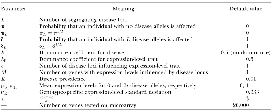
TABLE 1
Description of parameters
Parameter Meaning Default value
L Number of segregating disease loci —
p Probability that an individual with no disease alleles is affected 0
pL pL¼p1=L 0
d Probability that an individual withLdisease alleles is affected 1
dL dL¼d1=L 1
h Dominance coefficient for disease 0.5 (no dominance) hE Dominance coefficient for expression-level trait 0.5
c Number of disease loci influencing expression-level trait 1 M Number of genes with expression levels influenced by disease locus 1
K Disease prevalence 0.01
m0;m2c Mean expression levels for 0 and 2cdisease alleles, respectively 0, 1
sE Genotype-specific expression-level standard deviation 0.333 t m2cm0
s 3
treatment and controls, then that repetition is declared a success. The power is then approximately equal to the fraction of success in a large number of trials.
POWER TO DETECT EXPRESSION LEVEL DIFFERENCES DUE TO POLYMORPHISMS
BETWEEN AFFECTED AND UNAFFECTED INDIVIDUALS: RESULTS
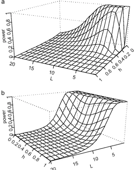
Reactive expression-level traits—multiplicative model: Dependence on h and L: Figure 1 shows surface plots of power to detect expression-level trait differ-ences vs. L(effective number of causative loci) and h
(dominance coefficient) for a multiplicative model. For each plot, disease prevalenceK¼0.01, expression-level trait standard deviationsE¼0:333, sample size is 200 (100 for each treatment), the penetrance parametersp
and d are 0.0 and 1, respectively (indicating perfect penetrance with respect to the full multilocus geno-type), and the expression-level trait depends only on a single TCL. Thus, there are three expression-level trait means. In both plotsm0 ¼0 andm2¼1:0, wheremi is
the mean expression level for individuals withidisease alleles at the TCL. These values correspond tot¼3. The dominance in expression is hE ¼ 0 (completely re-cessive) in Figure 1a and hE¼0.5 (no dominance) in Figure 1b. I assume that there are 20,000 genes tested on the microarray. These are default parameter values (withhE¼0.5) throughout this article unless otherwise specified.
The determinant of power is the amount of contrast between the treatment means. In Figure 1a, the expres-sion-level trait is recessive and there is no mean dif-ference between individuals withddandDdgenotype at the causative locus. Whenh¼0 (disease risk is recessive with respect to the TCL), then all affected individuals are DDat the TCL. When L ¼ 1, then all unaffected individuals areddorDdat the TCL and there is a strong contrast in expression level between the affected and unaffected treatments. The power is near 1. When h
moves away from 0, then some Ddindividuals are also affected. Because the disease allele is rare whenL¼1, most affected individuals are Ddwhenh .0 and thus there is little contrast between treatments. Thus, we see that the power quickly drops to near 0 ashis increased forL¼1.
WhenL .1, then some nondisease individuals will also haveDDgenotypes at the TCL (see the description of the multiplicative trait model). AsLis increased, the disease-allele frequency at the TCL also increases. As the number of causative loci is increased, then the proba-bility of the disease events associated with those loci must also increase to maintain the constraint that the disease prevalence is 0.01. For example, the disease-allele frequency is 0.68 forL¼6 and 0.75 forL¼10 at
h ¼0. See Schliekelmanand Slatkin(2002) for fur-ther details and plots of allele frequencies. As L in-creases, the proportion of unaffected individuals with a
DDgenotype at the TCL also increases. Thus, the con-trast between the two treatments also decreases and power drops quickly. Ath¼0.1, power is near 97% for
L¼6, but drops to46% forL¼11. The power also drops quickly ashis increased from 0. For example, at
h¼0.3, the power is,50% for all values ofLand forh$
0.5 the maximum power is 0.05. One interesting aspect of Figure 1a is that power actually increases when
Lis increased from 1 whenhis low but.0. This occurs because allele frequency increases asLis increased. As discussed above, the disease-allele frequency is low for
L ¼1 and when h . 0 most affected individuals are genotypeDd. The allele frequency increases asLdoes and thus more affected individuals are of genotypeDD. Only genotypeDDproduces any contrast in expression level, so power is increased.
Figure 1b has identical parameter values except that
hE¼0.5 (no dominance in expression). In this case, the power to detect differential expression is less sensitive to
hand does not drop to zero ashis increased. Power is lowest for intermediate h and as above is highest for
Figure1.—Plot of powervs. L(number of disease loci) and
h(the dominance coefficient). The power is the probability of rejecting the null hypothesis of no difference in expression between the treatments. Parameter values arep¼0,d¼1, K¼0.01, andsg ¼0:333, and the sample size is 100 for each
treatment. In both plotsm0¼0 andm2¼1:0, wheremiis the mean expression level for genotype withidisease alleles at the TCL. The dominance coefficient for expressionhE is 0 in a
h¼0. However, the power in the best case is substantially worse for largerL than in the previous example. The maximum power is 0.81 forL¼6 and 0.61 forL¼5. As discussed above, disease-allele frequency is quite high for largerLwhenh¼0. Thus, the difference between treatment groups is primarily due to differences between
Dd and DD individuals. Because the expression-level means are closer together, the difference is less. The closerh is to 0.5, the more affected individuals are of
Ddgenotype. Again, the contrast between treatments is lower and power decreases.
Supplemental material available at my website shows a similar plot for the case withhE¼1. In this case the power is highest ath¼1 and drops off quickly ashis decreased from 1 (although less quickly than in Figure 1a).
Dependence on c: Next, I explore how the number of loci (c) controlling the expression-level trait affects the power to detect an expression-level difference. The more similar the genotypic dependence of the expression-level trait is to that of the disease, the more contrast in expression-level trait we expect there to be between af-fecteds and unafaf-fecteds. Thus, increasing the number of loci controlling the expression-level trait should increase the power (since all loci controlling the expression-level trait are assumed to be controlling disease status also). There is no question that increasing the range of varia-tion in an expression-level trait will increase power. The unknown is how changing the control of expression level affects power. Therefore, the maximum and mini-mum expression levels are kept constant ascis varied. That is, the expression level for the genotype with allc
loci asDDis constant and the expression level for the genotype with allcloci asddis constant. Figure 2 shows plots for several parameter values. In Figure 2, a and b, the expression-level trait has an additive dependence on the TCLs while it has a multiplicative dependence in
Figure 2, c and d. In all cases the disease has a multipli-cative dependence. We see that the power increases only slowly withc in the additive case. The advantage of in-creasingcis that it increases the concordance of geno-typic dependence between expression-level trait and disease status. However, if disease and expression-level traits depend in fundamentally different ways on the multilocus genotype, this concordance does not in-crease substantially withc.
In Figure 2, c and d, we see the unexpected result that the power initially increases withc but then decreases. The increase is because of the increased concordance of control of disease and genotype. That is, it is quite likely that an unaffected individual will have one or two dis-ease alleles at a given locus ( just not at all loci). Thus, if
c¼1 then the ELT will often be differently regulated in unaffected individuals. It is less likely that the unaf-fected individual will have disease alleles at all of some set of multiple loci. Thus, the ELT is less likely to be differently regulated in unaffecteds whenc.1 and thus there is stronger association between disease and ELT and power initially increases withc(except forL¼3). The decrease occurs because of how the disease and expression models are defined. As c increases, it be-comes likely that multiple controlling loci for the ELT in affecteds will be heterozygotic. In Figure 2c, the con-tributions to the expression means fordd,Dd, andDD
individuals are 0, 0.5, and 1, respectively. Because these values are multiplied to get the mean, then the mean moves much closer to 0 than to 1 if there are more than one to two heterozygote loci. Thus, whencis large, then even affected individuals often have low expression means and this diminishes the contrast in expression between affected and unaffected. In Figure 2d,h is in-creased from 0.5 to 0.9. This leads to a dein-creased disease allele frequency (for constant K) and thus more
het-Figure2.—Plot of powervs. c
(num-ber of loci controlling expression-level trait). The y-axis is the probability of detecting a significant expression-level difference between affected and unaf-fecteds. The different curves corre-spond to the value ofL as shown in a (the order is the same for b–d). The power is the probability of rejecting the null hypothesis of no difference in expression between the treatments. In a and b the expression-level trait has an additive dependence on genotype, while there is a multiplicative depen-dence in c and d. The number of genes tested on the microarray was assumed to be 20,000. Parameter values arep¼0,
d ¼ 1, L ¼ 9, K ¼ 0.01, sg¼0:333,
m0¼0, he ¼0.5, andm2c ¼1. The
pa-rameter h ¼ 0.5 in a and c and h ¼
erozygote loci for affecteds. This in turn leads to more rapid loss of power asc increases. It is difficult to say whether this behavior is reasonable or should be considered an artifact of the model.
We see in Figure 2, c and d, that there is good power to detect expression-level differences forL¼3 andc¼1–2 and forL¼6 cases andc¼2–3. For higher values ofL
andh¼0.5 (Figure 2c) the power is maximized in the 50–60% range forc¼4–5. For theh¼0.9 case (Figure 2d) power is substantially lower.
Dependence on M (number of expression-level traits controlled by the TCL): If the difference in genotype distribution between affecteds and unaffecteds means is not large at the TCLs, then the probability of the sample means being different enough to achieve significance may be small. In this case, the probability of achieving significance is increased if there are multiple expression-level traits dependent on the TCLs. Figure 3 shows a surface plot of powervs. candMforL¼9,hE¼h¼0.5, and a sample size of 200. The power here is defined as the probability that at least one of theMELTs is detected as differentially expressed. Whenc¼1, we see the power increasing from 5% forM¼1 to 50% forM¼40. In this case, there is little distinction between affecteds and unaffecteds at the TCL. The disease-allele frequency is 0.6 for these parameter values. Approximately 84% (that is, 10.42) of unaffecteds carry a disease allele at
the TCL and there is little difference in TCL genotype between affecteds and unaffecteds. With so little differ-ence in genotype distribution, each additional ELT dependent on the TCL makes only a small difference. However, a large number of such ELTs do make a substantial difference. For the casec¼2, small changes inMhave a substantial affect on power. When we jointly consider two loci, the genotypic difference between treatments is greater. Power is still poor (36%) forM¼
1, but improves to.80% for M¼8. Forc¼3, power
increases from60 to90% whenMis increased from 1 to 4. Thus, increasedMcan help power substantially in cases where the genotypic distinction between treat-ments is intermediate.
Dependence on sample size: Figure 4 shows plots of power vs.sample size for various values ofMandcfor
L ¼9.M¼1 for all curves in Figure 4a, but varies in Figure 4b as shown. WhenM¼1, there is no case for which the power reaches 80% for sample sizes ,250. A sample size of 600 is required for 80% power when
c ¼1. The best case is 80% power for a sample size of 250 whenc¼3. The sample sizes become more reason-able (although still rather large) for higherM. Power is 85% and 92%, respectively, forc¼3 andM¼4 and 8 and a sample size of 160. However, a sample size of 350 is required to get 80% power even whenM¼8 forc¼1 or 8.
Dependence on penetrance parameters: All of the above plots had perfect penetrance for the full multilocus genotype (that is,p¼0 andd¼1). Figure 5 shows that varying p (the probability of an individual with no disease alleles being affected) from zero seriously decreases power, while decreasingdfrom 1 has negligi-ble effect. Forp $0.00005, the power is near zero even for a sample size of 1500. Whenp¼0 it is certain that an affected individual has at least one disease allele at each locus. Whenp.0, then some affected individuals do not have any disease alleles at some loci. For the pa-rameters in Figure 5 (L¼9 and prevalence¼0.01) and
p¼0.0005, it can be shown that most affected individ-uals have at least one locus with no disease alleles. Thus, the contrast in expression levels between affecteds and unaffecteds is diminished. On the other hand, many loci
Figure3.—Effect ofM. Thez-axis is the probability of
de-tecting a significant expression-level difference between affec-teds and unaffecaffec-teds for at least one of theMexpression-level traits plotted against the parameterscandM. Parameter val-ues are otherwise the same as those in Figure 2. The power calculations are based on simulations with 500 repetitions.
Figure4.—Plot of powervs.sample size. They-axis is the
in unaffected individuals have a disease alleles regard-less of the value ofdand changing it therefore has less effect. The sharp drop in power aspL is increased is largely due to the particular form of model used. The parameterpis the probability of an individual with no disease alleles being affected. The parameter pL, the contribution to disease risk of the TCL, is pL¼p1=L.
WhenL is large, pL increases very quickly asp does.
For example, when L ¼ 9 and p ¼ 0.0005, then
pL ¼0:00051=9¼0:43. Thus, the probability that a locus
with no disease alleles contributes its disease event is quite high. The effect of varyingdis small for the same reason. Ford¼0.5 andL¼9, the value ofdLis 0.51/9¼
0.93. It is, of course, unknown whether this form forpLis
appropriate. However, if we assume a multiplicative model and that individuals with no disease alleles can have the disease, then it is necessary.
Dependence on the heritability of expression-level trait: As the heritability of the expression-level trait with respect to the TCL increases, so does the power to detect that TCL. In the above results, I assumedðm2cm0Þ=s¼3, where m2c and m0 are the expression-level means for individuals with all 2c disease alleles and 0 disease alleles, respectively, andsis the standard deviation in gene expression. This corresponds to 45% of variance explained by genotype. Referring to supplemental Fig-ure 1, we see that a value of three is among the highest values calculated for the Hedenfalk data. However, there are genes with values ranging as high as six, and the power to detect expression level differences for these genes will be greater. Figure 6 shows a plot of power vs. the parameter t¼ ðm2cm0Þ=s for various values ofL and c. In this figure m2c and m0 are held constant at 1 and 0, respectively, while the
expression-level variancesis varied. The sample size is 200,h¼5,
hE¼0.5, and all other parameters are as in Figure 2. As expected, the power increases steadily with t. For example, the power in theL¼6,c¼1 case increases from7% att¼2 to 86% fort¼8. On the other hand, the power in theL¼9,c¼1 case reached only 37% at
t¼8 because it started from only 1%.
Natural population—additive model: Power under an additive penetrance model is substantially worse than that under a multiplicative model. Figure 7a shows a plot of power to detect expression-level differencesvs. Figure5.—The effect of penetrance parameters. They-axis
is the probability of detecting a significant expression-level difference between affecteds and unaffecteds. The curves cor-respond to different values of the penetrance parametersp
anddas shown.p¼0 andd¼1 except when otherwise in-dicated. Parameter values are otherwise the same as those in Figure 2.
Figure6.—The effect of the heritability of expression level.
They-axis is the probability of detecting a significant expression-level difference between affecteds and unaffecteds. Thex-axis is the value of the parametert¼ ðm2cm0Þ=s. The curves cor-respond to different valuesLandcas shown. Parameter values are otherwise the same as those in Figure 2.
Figure7.—Power for the additive penetrance model. The
sample size forL¼4 andL¼6 and a range ofcvalues for each. The power is very poor. With just four disease loci, sample sizes of.800 are required to reach 80% power. WhenL¼6, power is just 10% with an 800-sample size. Crucially, the power is not affected much byc. This is in contrast to the multiplicative model, where increas-ing c has a large effect on power. Under the additive model, the mean expression levels for affecteds and unaffecteds do not change ascis varied. A proof of this is given in the supplemental results. Power increases with
c under a multiplicative model (for small c) because increasingcincreases the concordance between expres-sion-level trait and disease. Under an additive model, each locus contributes independently and increasingc
does not increase the concordance.
Power under a multiplicative penetrance is much higher than that under additive penetrance even forc¼
1. This is due to the very different genotype distributions under the two models. With multiplicative penetrance, affected individuals have at least one disease allele at all loci (or at most loci if the penetrance parameterp.0). In contrast, only one locus need have a disease allele to cause disease with additive penetrance. WithL¼6 and other parameters as in Figure 7a, 90% of affected individuals carry only a single disease allele and most of the remaining 10% carry single disease alleles at two loci. Thus, only (90%/6110%/3)¼18% of affected individuals carry a disease allele on a given disease locus. Assuming no dominance as in Figure 7, the average expression level for a gene controlled by this locus is 0.5 and thus the average expression level among affecteds is 0.5 3 0.18 ¼ 0.09. Most unaffecteds carry no disease alleles, so the mean difference in expression level be-tween affected and unaffected is0.09. With the same parameters and a multiplicative model, affecteds on average have three loci that are homozygous for the disease allele and three loci that are heterozygous. The average expression level in affecteds for a gene con-trolled by the disease locus would be0.53110.53 0.5¼0.75. Now, as discussed earlier, disease-allele fre-quencies are high under a multiplicative model (in strong contrast to the case with an additive model). The
disease-allele frequency would be 0.46 for the parame-ters in Figure 7 and genotype frequencies in unaffecteds would be0.21 disease homozygote, 0.50 heterozygote, and 0.29 normal homozygote. Thus, the mean expres-sion level in unaffecteds would be 0.213110.530.51 0.29 3 0 ¼ 0.46 and the mean difference between affecteds and unaffecteds would be0.750.46¼0.29. The mean difference in expression level is 3.5 times higher for the multiplicative model than for the additive one and power to detect expression-level differences is correspondingly higher under the multiplicative model. Figure 7b shows a plot of powervs. Mfor sample size 200,L¼4, andc¼1, 3, and 5. We see increasingMhas minor impact. Even for this low value ofLthe power is still low forMup to 20.
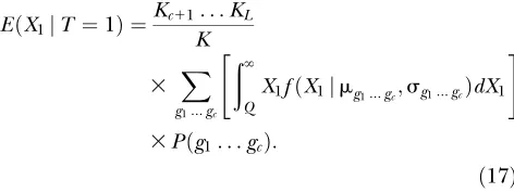
Causative expression-level trait:There are many pos-sibilities for how disease risk depends on the expression level of a causative transcript. I use a simple threshold model withu(X1)¼1 ifX1$Qandu(X1)¼0 ifX1,Q. The expression means and variances for affected and unaffected individuals are calculated using Equation 15 in a similar manner to that done for the reactive ELT. For example, the expected value among affecteds for the multiplicative model is
EðX1jT ¼1Þ ¼
Kc11. . .KL
K
3 X
g1...gc
ð‘
Q
X1fðX1jmg1...gc;sg1...gcÞdX1
" #
3Pðg1. . .gcÞ:
ð17Þ
Figure 8a shows a plot of power to detect a difference inX1between affecteds and unaffecteds as a function of sample size. The parameter Q ¼ 0.5, c ¼ 1, and the expression means arem0 ¼0,m1¼0:5, andm2¼1. The different curves correspond to the value ofLas shown. Other parameters are as in Figure 2. The power is greatly improved compared to a reactive ELT. For example, we see that 80% power is achieved at a sample size of100 whenL¼9. This compares to a sample size of 600 for
Figure8.—Power for causative ELT. They-axis
80% power for similar parameter values with a reactive ELT. This increased power results from a combination of higher expression means and lower variances for affected individuals when the ELT is causative relative to the case when it is reactive. Both of these effects result primarily from the heterozygote expression distribution being truncated in affected individuals. The value of the ELT must exceedQ in affected individuals. With the parameter values in Figure 8 (Q ¼0.5 andm1¼0:5), half of the expression distribution is truncated in af-fected heterozygotes.
Figure 8b shows the effect of the thresholdQ. We see that for these parameter values the power is at a peak at
Q¼0.6, but thatQhas a small impact on power. The effects of varying Q are complicated. As Q increases, fewer individuals will have an ELT value that exceeds it. Thus, the disease-allele frequency must increase to keep disease prevalence fixed. IncreasingQ has four major effects. First, it increases the expression mean in affected individuals, which tends to increase power. Second, it increases the expression mean in unaffected individuals (because the disease-allele frequency increases), which tends to decrease power. Third, increasingQreduces the portion of each genotype-specific expression distribution that exceeds the threshold, tending to decrease variance. Fourth, whenQreaches extreme values, then the disease allele frequency does also. This tends to reduce expres-sion variance by reducing genetic variance in the population. The interaction between these effects is complex, but the net effect on power is small because the various effects are often in opposition to each other. Figures available as supplemental material show the effects of various other parameters on the power for the causative ELT. Power increases very substantially withc
as the proportion of the risk explained by the ELT increases. The degree of dominance in the ELT (that is, the mean expression level for heterozygotes) has a roughly inverse effect to that ofQ. That is, power is at a peak for intermediate dominance and the various effects discussed above for Q work in roughly the opposite direction ashis increased.
AllowingMto vary for causative ELTs would require specifying a model for how these ELTs interact to determine disease risk. Thus, I keep M fixed at one. Other parameters have effects similar to those observed for reactive ELTs.
This model for a causative ELT is not compatible with additive disease risk for the standard parameter values used in this article. In the additive case, the disease risk associated with the causative locus isK/L ¼0.01/9 ¼
0.0011. Under the standard parameters, the ELT has a probability of 0.07 of exceeding the thresholdQ¼0.5 when its controlling locus has no disease alleles. This means that an individual with no disease alleles still has a probably 0.07 of being affected, which far exceeds the ‘‘allowed’’ disease risk for the locus. This can be cor-rected by lowering the genotype-specific ELT standard
deviationsEto a level that makes the probability of ex-ceedingQ,0.011. This requires halving the standard deviation to0.15 for the standard parameter values. Not surprisingly, power is quite good with this low ELT variance (comparable to that seen in Figure 8). How-ever, the analysis ofsEvalues described in themethods section indicates that ELTs with values this low may be very rare.
POWER TO MAP CAUSATIVE LOCI USING DIFFERENTIALLY EXPRESSED TRANSCRIPTS
AS QUANTITATIVE TRAITS
Above, I considered the power to detect differences in expression-level traits between disease-affected and -unaffected individuals. For causative ELTs, good power to detect association with the disease is achieved withc¼
1 and sample sizes of100. Withc¼1 (meaning that the ELT has a single controlling locus), the power to map the controlling locus will be good. Thus, in this case, eQTL-based strategies for genome scans should be powerful.
The situation is more complicated for reactive ELTs. Power was shown to be very poor if an additive pene-trance model holds. Power for multiplicative penepene-trance depends strongly on the parameterc. If there is only a single TCL controlling an expression-level trait (c¼1), then power to detect an association between that gene and disease status is low unlessLis small. If multiple TCL control the gene (i.e.,c. 1), then the power to detect associations with the disease is higher. However, this expression-level trait is then a multilocus trait and it will have lower power in use as a quantitative trait for de-tecting the TCL(s).
A number of methods for mapping QTL in natural populations have been proposed (see,e.g., Lynchand Walsh1998). I will focus on humans and assume that mapping is conducted using Haseman–Elston (HE) regression (Hasemanand Elston1972). HE regression uses sib pairs and detects linkage to a QTL by regression of the squared difference in trait values on the number of alleles identical-by-descent (IBD) between the sibs at each marker. If a marker is linked to a QTL, then there should be a negative correlation between the squared trait difference and the IBD status at the marker.
I used a Monte Carlo simulation to estimate power for HE regression with an eQTL. I assumed a multiplicative model for gene expression with equally contributing loci. Figure 9a shows a plot of powervs.the parameterc
for sample sizes of 100, 300, and 500 sib pairs.M¼1 in Figure 9a. That is, there is one expression-level trait controlled by the eQTL. This expression-level trait being tested is assumed to be completely linked to one of thec
against each of hundreds of markers (note that a cor-rection for 20,000 tests was used in previous sections of this article). We see that power drops quickly as c
increases, with,10% power forc¼2 and 500 sib pairs. The power to detect a causative locus is increased if it is an eQTL for multiple expression-level traits. That is, if there are M expression-level traits controlled by the locus then there are Mchances to detect it. However, these are not independent chances because the sample individuals are the same for each expression-level test. Thus, genotypes are not replicated. The expression-level traits are only independent conditioned on genotype.
The power curves in Figure 9b correspond toM¼10, 20, 50, and 100 as shown. The sample size is 500 sib pairs in each case. The power is defined as the probability that the target causative locus is detected as an eQTL for at least one of the expression-level traits. Each of the M
expression-level traits is assumed to be controlled by the same set ofcloci. We see that the power increases strongly withM. However, M¼100 is required to achieve 80% power whenc¼2 and the power is only 20% whenc¼3. The basic HE regression method assumed here is not the most powerful method available for detecting QTL in natural populations. However, other methods are not dramatically better and it is not expected that the qualitative results will be much different. Thus, we see that the power for detecting an eQTL is expected to be poor when the expression-level traits have more than one controlling locus, unless that locus is an eQTL for many expression-level traits.
DISCUSSION
There are too many unknowns to draw any firm conclusions about the likely effectiveness of mapping complex trait loci using gene expression levels as quantitative traits. There is strong evidence that a sub-stantial number of gene expression-level traits in many organisms have a relatively simple genetic basis and high heritability relative to that seen for complex clinical traits. Furthermore, Schadt et al. (2003), Brystrykh et al. (2005), Chessleret al.(2005), Hubneret al.(2005), and
others have identified probable associations of eQTL with clinical traits in mice or rats. Expression-level traits with high heritability will give good power for mapping their associated eQTL. However, I have shown here that establishing that these eQTL are also associated with the trait of interest may be difficult. If such expression-level traits are causative, in the sense of disease risk depending directly on expression level, then sample sizes on the order of 100 are sufficient for good power. On the other hand, if the ELT is reactive to a causative locus, then there is a trade-off between the power to show an association between expression-level trait and disease and the power to map eQTL for that expression-level trait. The simpler the genotypic dependence of an expression-level trait is on a disease-causative eQTL, the easier it is to map that eQTL. From a mapping perspective, the ideal case is that the expression-level trait depends on a single causative locus. However, in this case the correlation with the disease will be small. Most of the results in this article with
c¼1 andL. 3 for a reactive ELT show poor power to detect differential expression between affecteds and unaffecteds unless sample size is well over 500 individu-als. This power increases quickly ascdoes, although the sample sizes required for 80% power are all rather high compared to most current microarray experiments. Un-fortunately, the power to map causative loci drops quickly with c. Figure 9 shows that for Haseman–Elston re-gression the power to detect linkage is,10% forc.1 even with 500 sib pairs. This indicates that for humans there may be no expression-level traits that give good power both to detect reactive expression-level differences between affecteds and unaffecteds and to map their underlying causative loci. The underlying problem is that power is poor for mapping QTL in natural populations. This is somewhat ameliorated if the disease locus is an eQTL for many expression-level traits. However, there must be on the order of hundreds of controlled expression-level traits before power becomes reasonable. I stress again, however, that these power calculations are not meant to be taken too literally because there are many other possible methods for doing genome scans using eQTL. Thus, the results are intended more as a guide to intuition.
Figure9.—Power to map eQTL using Haseman–
Results that will appear in a future publication (P.
Schliekelman, unpublished results) show that the
situation is better for crosses with inbred lines. The power to detect expression-level differences is not sub-stantially higher, but the power to detect linkage drops off more slowly as the number of loci (c) controlling the expression-level trait increases.
These results do not imply that no reactive expres-sion-level changes should be detected with natural populations. On the contrary, the power to detect such differences is quite reasonable for expression-level traits influenced by multiple causative loci (i.e., expression-level traits with c . 1). The point is that the reactive expression-level traits that are found to be most differ-entially expressed are likely to be poor candidates for use as quantitative traits for linkage detection.
Model assumptions:The results of this article depend on a large number of assumptions about how disease risk and expression levels depend on genotype. This is unavoidable given our lack of knowledge of the genetics of complex traits. I have used two very different disease-penetrance models and a wide range of parameter values to give a sense of what the range of possibilities is. However, in the end the results of a model are only as good as the assumptions that go into it and it is possible that these assumptions are badly off.
In a sense, the additive and multiplicative models are at extreme ends of a continuum. A multiplicative model requires that each of the causative loci have a disease event for the disease to occur. The additive model requires only a single locus to have a disease event for disease to occur. As shown in this article, this difference results in very different genotype distributions. I have focused on the multiplicative model because the power to detect reactive expression-level differences is very poor under an additive model and the additive model does not appear consistent with a causative ELT. If an additive model is correct, then there appears to be little hope for mapping complex disease genes using eQTL. Fortunately, additive disease-penetrance models do not appear to be consistent with family history data in humans. Risch (1990) showed that inheritance patterns do not change as the number of causative loci increases under an additive model. Thus, if the inheritance patterns for a disease indicate a multilocus trait, then it cannot be additive. Multiplicative models typically do fit family history data well (e.g., Schliekelman and Slatkin 2002). However, it is likely that a great many other models would fit equally well and there is no way to tell if the ‘‘true’’ model behaves more like an additive model, like a multiplicative model, or like neither model.
The values ofM(the number of conditionally inde-pendent expression-level traits influenced by the TCL) assumed here are also highly speculative. Surveys of eQTL have found great variability in the number of gene expression-level traits mapping to individual loci.
Schadtet al.(2003) found several hotspots with
hun-dreds of eQTL mapping to 4-cM regions. Chesleret al. (2005) found a single locus modulating the expression of 1650 transcripts in addition to numerous loci mod-ulating hundreds of transcripts. On the other hand, Monks et al. (2004) did not find evidence of such hotspots. Their study was conducted with randomly chosen human families whereas studies that have found hotspots were conducted with inbred lines. One possi-ble explanation for the difference is that there is little variation at hotspot loci in natural populations, but selection for divergent phenotypes (or perhaps chance) in inbred lines leads to genotypic differences between strains. Another possibility is that expression-level traits with multilocus inheritance in natural populations become monogenic between inbred lines and thus are easier to detect. In any event, an increase inMincreases the power to detect at least one expression-level trait associated with the TCL and a causative locus with very highMwould be detectable as differentially expressed with reasonable sample sizes even forc¼1 (see Figure 3). However, Mis the effective number ofindependent
(given TCL genotype) expression-level traits influenced by the TCL. The amount of correlation between expression-level traits in the above studies is unknown. Most likely they are not all independent and the effective number of independent expression-level traits may be substantially lower than the observed number.
Comparisons to standard methods for genome scans:The required sample sizes shown here are large by the standards of typical microarray experiments, but not outrageous on the scale of human linkage studies. Power studies (e.g., Risch and Merikangas 1996;
Slager et al. 2000) have shown that sample sizes of
The results here show that the power to detect asso-ciation of a causative ELT with a disease locus compares very favorably with the power to detect complex trait loci using traditional mapping methods. Why should this be so? That is, the locus controlling the ELT in Figure 8 accounts for one-ninth of the disease risk. Numerous gene-mapping power studies show that the power to detect such a locus is poor. Why is the power apparently better to detect disease association with an ELT that accounts only for one-ninth of the risk? The answer to this can be understood by analogy with association studies for complex traits. It is well established (e.g., Rischand Merikangas 1996) that association studies are powerful for detecting common disease alleles when there are only two alleles in the population. However, power in association studies plummets when there are multiple alleles (Slageret al.2000). In detecting asso-ciation of a causative eQTL with a complex trait, the ELT is a proxy for genotype. If the genotype-specific expres-sion means were widely enough separated, then we could unambiguously assign individuals to groups cor-responding to genotype and conduct an association test directly. We do a similar thing when we do at-test of an ELT determined by a mixture of expression distribu-tions. We will tend to find a significant difference in expression between affecteds and unaffecteds if the allele frequency at the locus controlling the transcript is substantially different between affecteds and unaffec-teds, which is the same requirement for an association test. It can be shown (P. Schliekelman, unpublished data) that there are strong similarities between the functional forms of the noncentrality parameters that determine power for a case–control test and for at-test of an ELT determined by a mixture of genotype-specific expression distributions and that these tests have similar dependence on population genetic parameters. A key advantage of an ELT approach is that there are effec-tively only two allele types. That is, all alleles that in-crease expression (and therefore disease risk in this study) are collapsed into a single disease-risk-increasing group and all alleles that decrease expression are grouped into a risk-decreasing group. Thus, testing for an association between an ELT and a clinical trait has a strong similarity to association testing with just two alleles.
A key advantage of ELT-based methods is that they identify direct correlations to genes and not to markers. Even if the identified gene is reactive only to a disease locus and not disease causative, there is still is no recom-bination with a marker to diminish power. It appears that establishing association between transcripts and trait will be the low-power stage in genome scans using eQTL, while establishing linkage between a transcript and a marker will be relatively easy. Having no recombination involved in the low-power stage may be a major advantage for eQTL genome scans. Of course, there will also likely be genes whose expression level is controlled by a locus
linked to a disease locus and where recombination is a factor. Such genes will also be correlated with the disease, but more weakly if all else is the same.
Improvements in power: There appears to be sub-stantial potential for increasing the power of genome scans using eQTL beyond what I have shown here.
Schadt et al.(2003) stressed the importance of
com-bining information from all transcripts instead of focusing on transcripts individually as I have done here. Several studies (Ghazalpouret al.2005, 2006; Liet al. 2006) have used approaches that combine information from many transcripts in what are essentially genome scans. For example, Ghazalpouret al. (2006) identified 12 transcription modules using gene coexpression net-works constructed from expression data for 3421 genes in an F2cross between inbred mice strains. They then looked for correlations between these transcription modules and obesity-related clinical traits by calculating the average correlation between the traits and genes in the module. Finally, they mapped eQTL for all genes within the modules and looked for genomic regions that were enriched for eQTL for each module.cis-eQTL in these regions were then taken as candidate genes for traits correlated with the corresponding transcription module. For example, they found one module signifi-cantly correlated with body weight and nine genomic regions enriched for this module. One of the major advantages of this approach relative to the assumptions of the analysis presented here is that the gene module approach greatly reduces the number of tests for correlation (that is, from thousands down to 12). This greatly increases the power to detect a correlation with the trait. A potential drawback is that there is no way to tell whether a particular candidate region is causative for the trait or is causative only for the module. Still, this type of approach seems very promising.
Experimental designs utilizing family structure will reduce the number of segregating loci between affected and unaffected subjects and this can be used to increase power for detecting expression-level differences associ-ated with causative loci. Kraftet al.(2003) proposed a family-based test for correlation between gene expres-sion and a quantitative trait. They presented power simulations showing very good power for their proposed test, but did not model the genetics of the trait or expression level. Instead they assumed correlations of 33 or 67% between trait and expression level. The results here indicate that this assumed correlation is far too high for complex traits. While their method is promising, the power cannot be expected to be as high as their simulations show.