Texture Separation Using Enhanced
Morphological Component Analysis
Kapil Giri 1, Deepak Singh Rawat 2,Binay Kumar Panday 3, H. L. Mandoria 4
M.Tech Student, Department of Information Technology, G.B.P.U.A &T, Pantnagar, Uttarakhand, India1,2
Associate Professor, Department of Information Technology, G.B.P.U.A &T, Pantnagar, Uttarakhand, India 3
Professor, Department of Information Technology, G.B.P.U.A &T, Pantnagar, Uttarakhand, India 4
ABSTRACT: The Morphological Component Analysis (MCA) is a method which allows us to separate features contained in an image when these features present different morphological aspects. MCA can be used for image inpainting and image separation task. MCA can be very useful for decomposing images into texture and piecewise smooth(cartoon) parts. Due to the use of curvelet dictionary in MCA piecewise smooth content part suffers from ringing artifact. TV regularization scheme was used to remove ringing artifact from the piecewise smooth part.
In this work we aim at improving the MCA algorithm so that it can separate the piece wise smooth part and texture part more efficiently. The TV regularization scheme is approximated with daubechies wavelet. Daubechies wavelet transform is applied over the cartoon part of the image then soft thresholding of the coefficient is done and then again the image is reconstructed by taking inverse daubechies wavelet transform. Simulation result has shown that proposed method is giving better performance than the previous method in terms of various quality metric such as PSNR(peak signal to noise ratio), SSIM(Structural similarity).
KEYWORDS:MCA, Texture, Piecewise Smooth, Ringing Artifact, Wavelet.
I. INTRODUCTION
The Morphological Component Analysis (MCA) is a new method which allows us to separate features contained in an image when these features present different morphological aspects. MCA can be very useful for decomposing images into texture and piecewise smooth (cartoon) parts or for inpainting applications. MCA aims at separating these two parts on a pixel-by-pixel basis, such that if the texture appears in parts of the spatial support of the image, the separation should succeed in finding a masking map as a by-product of the separation process. In MCA, we base decomposition on sparse signal representation. MCA assumes that each signal is the linear mixture of several layers or morphological components that are morphologically distinct, such as sines and bumps.
Paper is organized as follows. Section II describes different types of Transforms, implementation method and algorithm. Section III. presents experimental results showing results of images tested. Finally, Section IV presents conclusion.
II. RELATED WORK
2.1Dictionaries for smooth content Wavelet transforms (WT)
The discrete wavelet transform (DWT) [19][20][21][25] is used in image processing to represent an image in the frequency domain. To begin the transform, the image is decomposed into four sub-bands and critically sub-sampled. The four sub-bands are – LL, LH, HL and HH. The four sub-bands arise from the separable application of vertical and horizontal filters. Wavelet transform inherently supports multi resolution analysis. Wavelet based codes have very good performance at low bit rates because trends anomalies and information at all scales in between are available.
The OWT implementation requires O(n2) operations for an image with n×n pixels, both for the forward and the inverse transforms. The OWT presents only a fixed number of directional elements independent of scales, and there is no highly anisotropic elements. Therefore, we expect the OWT to be non-optimal for detection of highly anisotropic features. Moreover, the OWT is non-shift invariance – a property that may cause difficulties in our analysis. The undecimated version (UWT) of the OWT is certainly the most popular transform for data filtering. It is obtained by skipping the decimation, implying that this is an over complete transforms represented as a matrix with more columns than rows.
The curvelet transform
The curvelet transform, proposed in [22, 23, 29] enables the directional analysis of an image in different scales. The idea is to first decompose the image into a set of wavelet bands, and to analyze each band with a local ridgelet transform. The curvelet transform is also redundant, with a redundancy factor of 16J + 1 whenever J scales are employed. Its complexity is of the O(n2log2n), as in ridgelet.
The curvelet decomposition is the sequence of the following steps i.e. Sub-band Decomposition and Ridgelet Analysis. The curvelet transform has a tight frame which combines multiscale analysis and ideas of geometry and can achieve optimal rate of convergence by simple thresholding[6]. This multiscale transform has a strong directional character in which elements are anisotropic at fine scales. The support of these elements obey the parabolic scaling principle length2=width. Traditional curvelet transform is based on the Ridgelet analysis theory, its digital realization is complicated and decomposition of Laplacian pyramid brings enormous date redundancy. The second generation curvelet transform (fast discrete curvelet transform) proposed by Candes et.al. provides two fast algorithms to implement it i.e. USFFT(unequally-spaced fast Fourier transforms) and Wrapping [26].
2.2Dictionaries for texture content The discrete cosine transform (DCT)
The DCT is a variant of the Discrete Fourier Transform, replacing the complex analysis with real numbers by a symmetric signal extension. The DCT is an orthonormal transform, known to be well suited for first order Markov stationary signals. When dealing with non stationary sources, DCT is typically applied in blocks. Such is indeed the case in the JPEG image compression algorithm. Choice of overlapping blocks is preferred for analyzing signals while preventing artifact.
A DCT expresses a finite sequence of data points in terms of a sum of cosine functions oscillating at different frequencies. The use of cosine rather than sine functions is critical in these applications: for compression, it turns out that cosine functions are much more efficient, whereas for differential equations the cosines express a particular choice of boundary conditions.
2.3 Implementation
calculating inverse wavelet transform original image is reconstructed. In next step discrete cosine transform of the residual is calculated.
After that two images are added which we get after calculating inverse discrete curvelet transform and inverse discrete cosine transform of the residual image. Than the sum will be reduced from the original image and it will be assigned as new residual. In next step residual image is added to the coefficient we get after calculating inverse curvelet transform earlier.
Again finding the curvelet transform of the resultant and repeat the previous steps. Results have been taken with total 30 iteration.
2.4 Algorithm
1. Initialize , number of iterations per layer N, and threshold = . .
2. Perform N times:
Part A - Update of assuming is fixed: Calculate the residual R = y – – .
Calculate the curvelet transform of + R and obtain
= ( + )
Soft threshold the coefficient with the threshold and obtain ἀ
Reconstruct by = .ἀ
Part B - Update of assuming is fixed: Calculate the residual R = y – – .
Calculate the local DCT transform of + R and obtain
= ( + )
Soft threshold the coefficient with the threshold and obtain ἀ
Reconstruct by = .ἀ
Part C - TV Consideration:
Apply the TV correction by = − { }
The parameter μ is chosen either by a line-search minimizing the overall
penalty function, or as a fixed step-size of moderate value that guarantees convergence.
3. Update the threshold by δ = δ – λ .
4. If δ > λ, return to Step 2. Else, finish.
A link between the TV and the undecimated Haar wavelet soft thresholding has been studied in [27], arguing that in the 1D case the TV and the undecimated single resolution Haar are equivalent. The TV introduces translation- and rotation-invariance, the undecimated 2D Haar presents translation- and scale-invariance (being multi-scale). J.-L. Starck , M. Elad , D.L. Donoho had approximated TV regularization scheme [18]with undecimated Haar wavelet transform and a soft thresholding But we have approximated TV regularization scheme with Daubechies wavelet and found that it is giving better result than tha haar wavelet.
Proposed Algorithm for TV Regularization
Calculate the Daubechies wavelet transform of and obtain ἀ .
Soft threshold the coefficient d with the threshold .
Reconstruct .by = ἀ .
So the TV correction is applied by using Daubechies wavelet transform.
2.5 Thresholding
The estimation of the true curve involves three steps. Apply Discrete Wavelet Transform (DWT) which transforms the discrete data from time domain into time-frequency domain. In the second step the wavelet coefficient are set to zero (hard threshold rule) or shrink (soft threshold rule), if they are not crossing certain threshold level. The last step is to reconstruct the signal from the resultant coefficient using Inverse Discrete Wavelet Transform (IDWT).
The estimation process involves these steps as follows
(1) Apply the two dimensional Discrete Wavelet Transform on the noisy data to obtain the sub-band approximate coefficients, horizontal details, vertical details and diagonal details. The orthogonal property of the transform insures that the noise in the transform is also of Gaussian nature.
(2) Threshold the detail coefficients using either soft or hard threshold rule.
For a given threshold λ > 0 the hard threshold value is given by Hard thresholding – It is a keep or kill procedure.
( , ) = ( > )
Soft thresholding – It is shrink or kill rule.
( , ) = ( − , 0)
2.6 Haar Wavelet
Hungarian mathematician Alfred Haar introduced Haar functions and they are used since 1910. After its origin, many definitions of the Haar functions, different generalizations [24] and some alterations were published and used. These transforms have been applied, for example, to spectral procedures for numerous valued logic, picture coding, edge extraction, and so forth. The non-sinusoidal Haar transform is the totally unitary transform. It can be used for data compression of non-stationary “spiky” signals for example digital images as it is local.
III. EXPERIMENTAL RESULTS
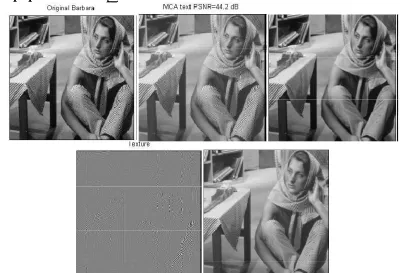
3.1 Results for Barbara image Result with MCA method for =10
Result with proposed method for =10
Fig. 2 2(a) shows the original image,2(b) image after adding image 2(c) and 2(d), 2(c) smooth part of the image 2(d) texture part of the image, 2(e) is showing the structural similarity.
We have applied the previous method and the new method over Barbara image. The texture and the cartoon part have been separated. We can see here that the new method is better than the previous one in terms of SSIM and PSNR. PSNR and SSIM are the image quality metric. For =10 previous method is giving PSNR = 41.6 while new proposed method is giving PSNR =44.2. So the proposed method is giving better result in terms of PSNR.SSIM value for previous method is 0.996 while SSIM value for the proposed method is 0.997. so our method is giving better result in terms of both the quality metric. so we can say that our method is separating the image into texture and cartoon part more efficiently than the previous method.
The table below shows effect on PSNR of the image when TV regularization scheme is approximated with Haar and Daubechies wavelet.
Gamma PSNR with Haar
PSNR with Daubechies 10 41.6 44.2 12 42.7 45.7 15 43.8 47.2
Table 1 Effect on PSNR
The table below shows effect on SSIM of the image when TV regularization scheme is approximated with Haar and Daubechies wavelet.
Gamma SSIM with Haar
SSIM with Daubechies 10 0.996 0.997 12 0.997 0.997 15 0.997 0.998
We have applied MCA algorithm over Barbara image. MCA has separated Barbara image into its texture part and natural scene part. Image was affected by ringing effect due to the curvelet transform of the image so the TV regularization scheme was applied to remove the ringing effect.TV regularization scheme works well when it is approximated with Daubechies wavelet instead of Haar wavelet. MCA show better PSNR when TV regularization scheme is approximated with Daubechies wavelet.
Fig. 3
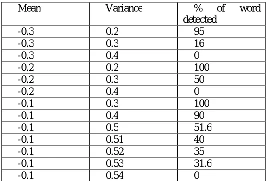
Tesseract OCR engine was able to read all the words correctly of the image show in fig.3.When we added different amount of noise to the above image than we got different results. We have added Gaussian noise to the above image, sometimes tesseract was able to read all the words and sometimes it can’t even able to read a single word.
Mean Variance % of word detected
-0.3 0.2 95 -0.3 0.3 16 -0.3 0.4 0 -0.2 0.2 100 -0.2 0.3 50 -0.2 0.4 0 -0.1 0.3 100 -0.1 0.4 90 -0.1 0.5 51.6 -0.1 0.51 40 -0.1 0.52 35 -0.1 0.53 31.6 -0.1 0.54 0
Fig. 4 shows the percentage of detected words by the OCR engine with fix variance
Fig. 4 shows the graph between numbers of words detected and mean of the Gaussian noise. The value of noise variance is fixed. Green line show the graph when noise variance is fixed at 0.02 and red line show the word detected by OCR engine when noise variance is fixed at 0.03.
So, proposed method has improved the performance of MCA algorithm in terms of PSNR and SSIM. Noise mean Noise
variance
PSNR with Haar
PSNR with Daubechies
% of detected words with MCA
% of detected words with proposed method -0.3 0.04 29.5 33.7 100 100 -0.4 0.03 32.1 36.2 96.66 98.33 -0.45 0.02 33.8 37.9 93.33 95 -0.5 0.02 35.6 39.1 91.6 98.3 -0.6 0.02 38.9 45.1 90 98.3
Table 5
IV. CONCLUSION
The proposed scheme is giving better result than the previous scheme. We have compared the performance of MCA algorithm and the proposed algorithm over two different types of images (Barbara image and text image) and found that proposed method is giving better performance than the previous one in terms of PSNR and SSIM.
Proposed scheme can also be used as a preprocessing step for optical character recognition engine. After preprocessing the text image, OCR engine is able to detect more number of correct words. Proposed scheme can be coupled with the optical character recognition engine.
REFERENCES
[1] Starck, J.L., Elad, M. and Donoho, D., 2004. Redundant multiscale transforms and their application for morphological component
separation. Advances in Imaging and Electron Physics, 132, pp.287-348.
[2] Starck, J.L., Elad, M. and Donoho, D.L., 2005. Image decomposition via the combination of sparse representations and a variational
approach. IEEE transactions on image processing, 14(10), pp.1570-1582.
[3] Vese, L.A. and Osher, S.J., 2003. Modeling textures with total variation minimization and oscillating patterns in image processing. Journal of scientific computing, 19(1), pp.553-572.
[4] Guo, C.E., Zhu, S.C. and Wu, Y.N., 2003, October. Towards a mathematical theory of primal sketch and sketchability. In Computer Vision,
2003. Proceedings. Ninth IEEE International Conference on (pp. 1228-1235). IEEE.
[5] Chen, S.S., Donoho, D.L. and Saunders, M.A., 2001. Atomic decomposition by basis pursuit. SIAM review, 43(1), pp.129-159.
[6] Starck, J.L., Donoho, D.L. and Candès, E.J., 2003. Astronomical image representation by the curvelet transform. Astronomy &
Astrophysics, 398(2), pp.785-800.
[7] Aujol, J.F., Aubert, G., Blanc-Féraud, L. and Chambolle, A., 2003. Image decomposition: Application to textured images and SAR
images (Doctoral dissertation, INRIA).
[8] Aujol, J.F. and Chambolle, A., 2005. Dual norms and image decomposition models. International Journal of Computer Vision, 63(1),
pp.85-104.
[9] Meyer, Y., 2001. Oscillating patterns in image processing and nonlinear evolution equations: the fifteenth Dean Jacqueline B. Lewis
memorial lectures (Vol. 22). American Mathematical Soc..
[10] Radin, L., Osher, S. and Fatemi, E., 1992. Non-linear total variation noise removal algorithm. Phys D, 60, pp.259-268.
[11] Gao, X., Wang, Y., Li, X. and Tao, D., 2010. On combining morphological component analysis and concentric morphology model for
mammographic mass detection. IEEE Transactions on Information Technology in Biomedicine, 14(2), pp.266-273.
[12] Hyvärinen, A., Karhunen, J. and Oja, E., 2004. Independent component analysis (Vol. 46). John Wiley & Sons.
[13] Prasad, R., Saruwatari, H. and Shikano, K., 2005. Blind separation of speech by fixed-point ICA with source adaptive negentropy
approximation. IEICE transactions on fundamentals of electronics, communications and computer sciences, 88(7), pp.1683-1692.
[14] Hyvärinen, A., Karhunen, J. and Oja, E., ICA by Minimization of Mutual Information. Independent Component Analysis, pp.221-227.
[15] Naik, G.R. and Kumar, D.K., 2011. An overview of independent component analysis and its applications. Informatica, 35(1).
[16] Fadili, J.M., Starck, J.L., Elad, M. and Donoho, D., 2010. MCALab: Reproducible research in signal and image decomposition and
inpainting. IEEE Computing in Science and Engineering, 12(1), pp.44-63.
[17] Hyvärinen, A. and Oja, E., 2000. Independent component analysis: algorithms and applications. Neural networks, 13(4), pp.411-430.
[18] Beck, A. and Teboulle, M., 2009. Fast gradient-based algorithms for constrained total variation image denoising and deblurring
problems. IEEE Transactions on Image Processing, 18(11), pp.2419-2434.
[19] Starck, J.L., Fadili, J. and Murtagh, F., 2007. The undecimated wavelet decomposition and its reconstruction. IEEE Transactions on Image
Processing, 16(2), pp.297-309.
[20] Mallat, S., 1999. A wavelet tour of signal processing. Academic press.
[21] Cohen, A., 2003. Numerical analysis of wavelet methods (Vol. 32). Elsevier.
[22] Donoho, D.L. and Duncan, M.R., 2000. Digital curvelet transform: strategy, implementation and experiments.
[23] Starck, J.L., Candès, E.J. and Donoho, D.L., 2002. The curvelet transform for image denoising. IEEE Transactions on image
processing, 11(6), pp.670-684.
[24] Struzik, Z. and Siebes, A., 1999. The Haar wavelet transform in the time series similarity paradigm. Principles of Data Mining and
Knowledge Discovery, pp.12-22.
[25] Garofalakis, M. and Gibbons, P.B., 2002, June. Wavelet synopses with error guarantees. In Proceedings of the 2002 ACM SIGMOD
international conference on Management of data (pp. 476-487). ACM.
[26] Candes, E., Demanet, L., Donoho, D. and Ying, L., 2006. Fast discrete curvelet transforms. Multiscale Modeling & Simulation, 5(3),
pp.861-899.
[27] Wang, Z., Bovik, A.C., Sheikh, H.R. and Simoncelli, E.P., 2004. Image quality assessment: from error visibility to structural similarity. IEEE
transactions on image processing, 13(4), pp.600-612.
[28] Eikvil, L., 1993. Optical character recognition. citeseer. ist. psu. edu/142042. html.
[29] Candes, E.J. and Donoho, D.L., 2000. Curvelets: A surprisingly effective nonadaptive representation for objects with edges. Stanford Univ