Optimization of Single and Multi Response
Characteristics in Machining of Mildsteel and
EN24 Using Taguchi and Desirability
Function Analysis (DFA)
Duggam Pradeep Saikumar 1, M.Balaji 2, Ismail Kakaravada 3, Y.Bhargavi 4
PG Student, Annamacharya Institute of Technology and Sciences (AITS), Tirupati, Andhra Pradesh, India1
Assistant professor, Department of Mechanical Engineering, (AITS), Tirupati, Andhra Pradesh, India2
Research Scholar, SVCET Research Centre, JNTUA, Andhra Pradesh, India3
Research scholar, S.V. University, Tirupati, Andhra Pradesh, India4
ABSTRACT: This paper presents in-depth and comprehensive approach for optimizing the machining parameters on Drilling of EN24 and Mild Steel using Taguchi method and Desirability Function Analysis (DFA).In various industrial applications, EN24 and Mild Steel are used for manufacturing of components such as gears, shafts, studs and bolts. In other hand, drilling is one of the most important cutting operations, comprising approximately 33% of all metal-cutting operations among all traditional machining processes. Among the metal-cutting conditions which influence the Drilling process, coolant is an important factor largely affects the machining process. The modern industries are looking for a cooling system to provide dry or near dry, clean, neat and pollution free machining. The present work is carried out in three phases; in the first phase the Orthogonal Array L32 Taguchi mixed level design is prepared using
Minitab software by considering various drilling parameters such as speed, feed, tool materials, work material and Coolant Type. In the second phase, drilling operation is performed on EN 24 and Mild Steel materials as per Taguchi design and the responses such as Thrust force, Torque, Temperature, Hole surface roughness and material removal rate (MRR) are obtained. In the third phase the experimental response data are analysed using Taguchi technique and Desirability Function Analysis. Using Taguchi technique optimum controllable parameter combinations are identified for each response. In view of the fact, that traditional Taguchi method cannot solve a multi-objective optimization problem; to overcome this limitation Desirability Function Analysis has been coupled with Taguchi method. Desirability function analysis (DFA) had been most widely used in industries to optimize the multi response in drilling operation and Drilling responses are analysed using this technique and optimum controllable parameter combination is identified and the significant contribution of parameters can be determined by analysis of variance (ANOVA). Finally optimal result was verified through confirmatory experiment and it is to be satisfactory.
KEYWORDS:Optimization, Drilling, Taguchi, Desirability function analysis (DFA), analysis of variance (ANOVA).
I. INTRODUCTION
Hole making is the most important operations in manufacturing. Drilling is a major and common hole making process. Drilling is the cutting process of using a drill bit in a drill to cut or enlarge the holes in solid materials, such as wood or metal. It is most frequently performed in material removal and is used as a preliminary step for many operations, such as reaming, tapping and boring.
tools, but high production machining with high cutting speed, feed and generates large amount of heat and temperature at the chip-tool interface which ultimately reduces dimensional accuracy, tool life and surface integrity of the machined component. This temperature needs to be controlled at an optimum level to achieve better surface finish and ensure overall machining economy. The conventional types and methods of application of cutting fluid have been found to become less effective with the increase in cutting velocity and fee when the cutting fluid cannot properly enter into the chip-tool interface to cool and lubricate the interface due to bulk plastic contact of the chip with the tool rake surface. It requires serious concern on the use of cutting fluid, particularly oil-based type cause for pollution of the working environment, water pollution, soil contamination and possible damage of the machine tool slide ways by corrosion [1]. The modern industries are therefore looking for possible means of dry (near dry), clean, neat and pollution free machining and grinding. Minimum Quantity Lubrication (MQL) refers to the use of cutting fluids of only a minute amount-typically of a flow rate of 50-500 ml/hour-which is about three to four orders of magnitude lower than the amount commonly used in flood cooling, for example, up to 10 litres of fluid can be dispensed per minute. The concept of Minimum Quantity Lubrication (MQL), sometimes referred to as ‗near dry lubrication ‘or ‗micro lubrication’.
Machining under minimum quantity lubrication (MQL) condition is perceived to yield favourable machining performance over dry or flood cooling condition. [2, 3, 4]
Basically, traditional experimental design procedures are too complicated and not easy to use. A large number of experimental works have to be carried out when the number of process parameters increases. To solve this problem, the Taguchi method uses a special design of orthogonal arrays to study the entire parameter space with only a small number of experiments. Using Taguchi technique optimum controllable parameter combinations are identified for each response [5, 6]. In view of the fact, that traditional Taguchi method cannot solve a multi-objective optimization problem; to overcome this limitation Desirability Function Analysis has been coupled with Taguchi method. Desirability function analysis (DFA) had been most widely used in industries to optimize the multi response process characteristics into single response characteristics. The advantage of the above method is that many factors can be analyzed using less data. It does not involve complicated mathematical theory or computations like traditional approaches and thus can be employed by engineers without strong statistical background [7-10].
From literature review it has been observed that Taguchi methodology can be applied to for analyzing the process parameters for single performance characteristics only , where as Desirability function analysis (DFA) can be effectively used for analyzing the multi performance characteristics incorporating the above all parameters at a time. The main objective of the present work is to investigate the effect of cutting parameters on predicted responses for drilling of EN24 steel and Mild steel using Taguchi – Desirability analysis approach under MQL condition environments and the experimental data was statistically surveyed by analysis of variance (ANOVA) to investigate the most influencing parameters on Thrust force, Torque, Temperature, Hole surface roughness and Material Removal rate (MRR).
II. METHODOFOPTIMIZATION
There are a number of techniques for optimization of output characteristics and to obtain optimum value but from all the optimization techniques, Taguchi's method for experimental Design is straightforward and easy to apply to many engineering situations, making it a powerful even simple tool. it can be used to quickly narrow down the scope of a research project or to identify problems in a manufacturing process from data already in existence. Also, the Taguchi method allows for the analysis of many different parameters without a prohibitively high amount of experimentation. It also allows for the identification of key parameters that have the most effect on the performance characteristic value so that further experimentation on these parameters can be performed and the parameters that have little effect can be ignored [8].
A. Taguchi Method
by process improvement. Taguchi has placed great emphasis on the importance of minimizing variation as the primary means of improving quality. Taguchi defines the quality level of a product to be the total loss incurred by society due to the failure of the product to deliver the expected performance and due to harmful side effects of the product, including the operating cost. In the concept some loss is unavoidable from the time a product is served to the customer and smaller loss provides desirable products. It is very important to quantify this loss for comparing various products Designs and manufacturing processes. This is done with a quadratic loss function. In the usual practice of manufacturing quality control the producer specifies a target value of the performance characteristic and a tolerance interval around that value. Any value of the performance characteristic of which is within the tolerance range about 3σ
is defined to be desirable product. With the loss function as a definition of quality the emphasis is on achieving the target value of the performance characteristic and deviations from that value are penalized. The greater deviation from the target value results with a greater quality loss. It seeks an answer that is insensitive to factor variations and noise.
1) Signal to noise (S/N) ratio: In the Taguchi method, the term ‘signal’ represents the desirable value (mean) for the output characteristic and the term ‘noise’ represents the undesirable value (standard deviation) for the output characteristic. The S/N ratio measures the sensitivity of the quality characteristic being investigated in a controlled manner to those external influencing factors (noise factors) not under control. So, Taguchi uses the S/N ratio to measure the quality characteristic deviating from the desired value. There are mainly three S/N ratios available depending on type of characteristic; lower-is better, nominal-is-best, or higher-is-better [9].
The Smaller-The-Better
For minimum surface roughness smaller-is-better is preferred, so the smaller is better quality characteristics can be explained as:
S
N = −10log
∑y n
The Larger-The-Better
For maximum material removal rate (MRR) Larger-is-better is preferred, so the larger is better quality characteristics can be explained as:
S
N= −10log 1 n∑
1 y
where , n = number of measurements in a trial/row, and yi is the ith measured value in a run/row.
B. Desirability Function Analysis (DFA)
From literature it has been observed that Taguchi methodology can be applied to for analyzing the process parameters for single performance characteristics only , where as Desirability function analysis can be effectively used for analyzing the multi performance characteristics incorporating the above all parameters at a time.
One useful approach for optimization of multiple responses is to use the simultaneous optimization technique popularized by Derringer and Suich (1980). Their procedure introduces the concept of desirability functions. The method makes use of an objective function, D(X), called the desirability function and transforms an estimated response into a scale free value ( ) called desirability. The desirable ranges are from zero to one (least to most desirable, respectively). The factor settings with maximum total desirability are considered to be the optimal parameter conditions.
Optimization steps using desirability functional analysis
STEP 1: Calculate the individual desirability (di) for the corresponding responses using the formula proposed by
Derringer and Suich. There are three forms of the desirability functions according to the response characteristics.
(a) The nominal-the-best: The value of ŷ is required to achieve a particular target T. when the ŷ equals to T, the desirability value equals to 1; if the departure of ŷ exceeds a particular range from the target, the desirability value equals to 0, and such situation represents the worst case. The desirability function of the nominal-the-best can be written as:
(ŷ ) , ≤ ≤ , s≥0
= (ŷ ) , ≤ŷ≤ , t≥0
0
Where the ymax and ymin represent the upper and lower tolerance limits of ŷ and s and t represent the indices.
(b) The larger-the-better: The value of ŷ is expected to be the larger the better. When the ŷ exceeds a particular criteria value, which can be viewed as the requirement, the desirability value equals to 1; if the ŷ is less than a particular criteria value, which is unacceptable, the desirability equals to 0. The desirability function of the larger-the-better can be written as:
0, ŷ≤
= (
ŷ
) , ≤ ŷ≤ , ≥0
1, ŷ≥
Where the ymin represents the lower tolerance limit of ŷ, the ymx represents the upper tolerance limit of ŷ and r
represents index.
(c)The smaller-the-better: The value of ŷ is expected to be the smaller the better. When the ŷ is less than a particular criteria value, the desirability value equals to 1; if the ŷ exceeds a particular criteria value, the desirability value equals to 0. The desirability function of the smaller-the-better can be written as:
1, ŷ≤
= ( ŷ ) , ≤ŷ≤ , ≥0
Where the ymin represents the lower tolerance limit of ŷ, the ymax represents the upper tolerance limit of ŷ and r
represents the weight. The s, t and r in above Equations indicate the weights and are defined according to the requirement of the user. If the corresponding response is expected to be closer to the target, the weight can be set to the larger value; otherwise, the weight can be set to the smaller value.
STEP 2: The individual desirability values have been accumulated to calculate the overall desirability, using the following equation (k). Here Dgis the overall desirability value, diis the individual desirability value of ith quality
characteristic and n is the total number of responses.
Dg = ( ∗ ∗ … … … … ) /
Here, Dg = Composite Desirability;
In the present work, the larger-the-better characteristic is applicable to determine the individual desirability values for Material removal rate (MRR) and the smaller-the-better characteristic is applicable to determine the individual desirability values for Temperature, Torque, thrust force and surface roughness.
STEP 3: Determine the optimal parameter and its level combination. The higher composite desirability value implies better product quality. Therefore, on the basis of the composite desirability (Dg), the parameter effect and the optimum level of each controllable parameter estimated.
STEP 4: Performing Analysis of variance (ANOVA) for the most significant parameter. ANOVA establishes relative significance of parameters. The calculated total sum of square values is used to measure the relative influence of the parameter.
STEP 5: The final step is to predict and verify the quality characteristics using the optimal level of the design parameters.
III.EXPERIMENTALDETAILS
For conducting this study a vertical Radial drilling machine is used as shown in figure 1. Work materials used in this study are EN24 and Mild steel. EN-24 is aNi-Cr-Mo (nickel chromium molybdenum) alloy steel with high strength and toughness and EN stands for Euronorms. It is normally suppliedas rolled, annealed, and hardened and tempered in the form of black round or square bar and bright round or square and hexagons .Carbon steel is sometimes referred to as 'mild steel' or 'plain carbon steel'. The American Iron and Steel Institute defines a carbon steel as having no more than 2 % carbon and no other appreciable alloying element. It can be case-hardened to improve wear resistance. It is supplied in bright rounds, squares and flats, and hot rolled rounds. Size of the material: 200x50x15mm.
The tool materials used in this study are HSS, HSS with 5%cobalt, HSS with 8%cobalt and HSS with TIN coated twist drills are shown in figure 2.The process parameters and their levels are summarized in Table 1.The responses consider in this study were Torque, Thrust force, Temperature, Surface roughness, MRR (metal removal rate). Surface roughness and MRR are considered as main quality and quantity responses. Torque and Thrust forces produced during drilling experiments is measured using drill tool dynamometer. The surface roughness is measured using stylus type (Mitutoyo Corporation, Japan) Talysurf (SJ-201 P) surface roughness measuring instrument. This temperature is measured using infrared pyrometer and MRR calculated by time and weight factors taken at the time of experimental run.
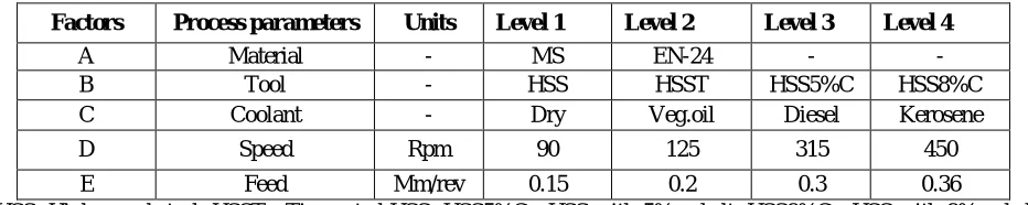
Table 1: Parameters and their levels
Factors Process parameters Units Level 1 Level 2 Level 3 Level 4
A Material - MS EN-24 - -
B Tool - HSS HSST HSS5%C HSS8%C
C Coolant - Dry Veg.oil Diesel Kerosene
D Speed Rpm 90 125 315 450
E Feed Mm/rev 0.15 0.2 0.3 0.36
Figure 1: Experimental setup of drilling experiments Figure 2: Drill tools (a) HSS with 8% cobalt (b) Tin coated HSS (c) HSS (d) HSS with 5% cobalt
Non-traditional machining including ultrasonic machining, abrasive water jet cutting, electrochemical machining (ECM), and chemical machining (CHM) are some of the example but conventional drilling still remains one of the most common machining processes (figure 1). For conducting this study a vertical Radial drilling machine is used as shown in figure 1. The tool materials used in this study are HSS, HSS with 5%cobalt, HSS with 8%cobalt and HSS with TIN coated twist drills are shown in figure 2. HSS is used as cutting tool material where the tool geometry and mechanics of chip formation are complex, such as helical twist drills, reamers, gear shaping cutters, hobs, form tools, broaches etc., and 5 % cobalt high speed steel for super abrasive resistance in tough metals, high speed steel bars with 8% cobalt achieving a hardness of some 63.5 - 65 Rockwell, Titanium nitride (TiN) (sometimes known as “Tinite” or “TiNite” or “TiN”) is an extremely hard ceramic material, often used as a coating on titanium alloys, steel, carbide, and aluminium components to improve the substrate's surface properties. Work pieces (Mild steel and EN 24) after drilling Operation is shown in figure 3.
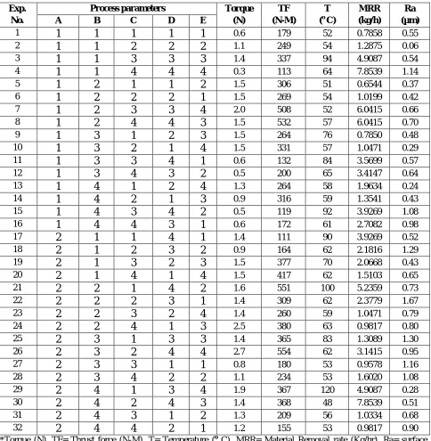
In this study, an orthogonal array L32 based on Taguchi method mixed level design was applied to design of
experiments. L32 orthogonal array (Experimental plan) and experimental results (responses) are summarized in table 2.
The experiments are conducted as per Taguchi L32 orthogonal array and work piece after drilling Operation is shown in
figure 3.
Table 2: L32 Orthogonal array (Experimental plan) and drilling responses
Exp. No.
Process parameters Torque (N)
TF (N-M)
T (o C)
MRR (kg/h)
Ra (µm) A B C D E
1
1
1
1
1
1
0.6 179 52 0.7858 0.552
1
1
2
2
2
1.1 249 54 1.2875 0.063
1
1
3
3
3
1.4 337 94 4.9087 0.544
1
1
4
4
4
0.3 113 64 7.8539 1.145
1
2
1
1
2
1.5 306 51 0.6544 0.376
1
2
2
2
1
1.5 269 54 1.0199 0.427
1
2
3
3
4
2.0 508 52 6.0415 0.668
1
2
4
4
3
1.5 532 57 6.0415 0.709
1
3
1
2
3
1.5 264 76 0.7850 0.4810
1
3
2
1
4
1.5 331 57 1.0471 0.2911
1
3
3
4
1
0.6 132 84 3.5699 0.5712
1
3
4
3
2
0.5 200 65 3.4147 0.6413
1
4
1
2
4
1.3 264 58 1.9634 0.2414
1
4
2
1
3
0.9 316 59 1.3541 0.4315
1
4
3
4
2
0.5 119 92 3.9269 1.0816
1
4
4
3
1
0.6 172 61 2.7082 0.9817
2
1
1
4
1
1.4 111 90 3.9269 0.5218
2
1
2
3
2
0.9 164 62 2.1816 1.2919
2
1
3
2
3
1.5 377 70 2.0668 0.4320
2
1
4
1
4
1.5 417 62 1.5103 0.6521
2
2
1
4
2
1.6 551 100 5.2359 0.7322
2
2
2
3
1
1.4 309 62 2.3779 1.6723
2
2
3
2
4
1.4 260 59 1.0471 0.7924
2
2
4
1
3
2.5 380 63 0.9817 0.8025
2
3
1
3
3
1.4 365 83 1.3089 1.3026
2
3
2
4
4
2.7 554 62 3.1415 0.9527
2
3
3
1
1
0.8 180 53 0.9578 1.1628
2
3
4
2
2
1.1 234 53 1.6020 1.0829
2
4
1
3
4
1.9 367 120 4.9087 0.2830
2
4
2
4
3
1.4 368 48 7.8539 0.5131
2
4
3
1
2
1.3 209 56 1.0334 0.6832
2
4
4
2
1
1.2 155 53 0.9817 0.90IV.RESULTSANDDISCUSSION
Taguchi methodology applied for analyzing the process parameters for single performance characteristics, Desirability function analysis used for analyzing the multi performance characteristics incorporating the all parameters at a time and ANOVA for identifying most significant parameter. The experiments are conducted as per Taguchi L32 orthogonal
array and work piece after drilling Operation is shown in figure 3 i.e., Drilled samples of mild steel and EN 24 steel specimens. After taking all the responses from Taguchi’s L32 orthogonal array, Taguchi methodology, Desirability
function analysis and ANOVA applied for optimization of machining parameters.
A. Results from Taguchi method
Taguchi's method for experimental Design is straightforward and easy to apply to many engineering situations, making it a powerful even simple tool. it can be used to quickly narrow down the scope of a research project or to identify problems in a manufacturing process from data already in existence.
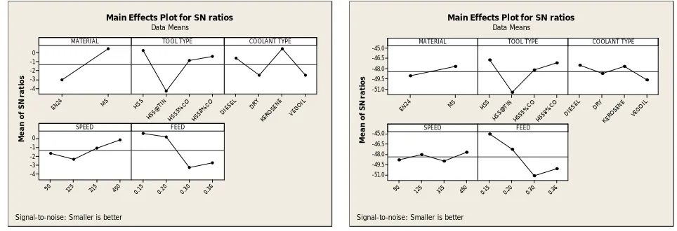
The responses consider in this study were Torque, Thrust force, Temperature, Surface roughness, MRR (metal removal rate). Surface roughness and MRR are considered as main quality and quantity responses. Torques, Thrust force, Temperature and Surface Roughness (Ra) are output character in drilling process and is to be minimized. Hence smaller the better S/N ratio is applicable for analyzing this character so the smaller the better formulae is used to analyze. Material Removal Rate (MRR) is an output character in drilling process and is to be maximized. Hence larger the better S/N ratio is applicable for analyzing this character. The main effect for mean and S/N proportion graphs are shown 4-8, respectively. Maximum levels of the S/N ratios of each controlled factors will give the optimum performance characteristic. MS EN24 0 -1 -2 -3 -4 HSS 8%C O HSS 5%C O HSS@ TIN
HSS
VEG
OIL
KERO
SEN
E
DRY
DIES EL 450 315 125 90 0 -1 -2 -3 -4 0.36 0.30 0.20 0.15 MATERIAL M e a n o f S N r a ti o s
TOOL TYPE COOLANT TYPE
SPEED FEED
Main Effects Plot for SN ratios
Data Means
Signal-to-noise: Smaller is better
MS EN24 -45.0 -46.5 -48.0 -49.5 -51.0 HSS8 %CO HSS5 %CO HS S@T IN HSS VEG OIL
K ERO
SEN E DRY DIE SEL 450 315 125 90 -45.0 -46.5 -48.0 -49.5 -51.0 0.36 0.30 0.20 0.15 MATERIAL M e a n o f S N r a ti o s
TOOL TYPE COOLANT TYPE
SPEED FEED
Main Effects Plot for SN ratios
Data Means
Signal-to-noise: Smaller is better
Figure 4: S/N Ratio Response graph of Torque Figure 5: S/N Ratio Response graph of Thrust Force
MS EN24 -35 -36 -37 HSS 8%CO HSS 5%CO HSS@ TIN HSS VEG OIL KER OSE NE DRY DIES EL 450 315 125 90 -35 -36 -37 0.36 0.30 0.20 0.15 MATERIAL M e a n o f S N r a ti o s
TOOL TYPE COOLANT TYPE
SPEED FEED
Main Effects Plot for SN ratios Data Means
Signal-to-noise: Smaller is better
MS EN24 8 6 4 2 HSS 8%CO HSS 5%CO HSS@ TIN HSS VEG OIL KERO SENE DRY DIES EL 450 315 125 90 8 6 4 2 0.36 0.30 0.20 0.15 MATERIAL M e a n o f S N r a ti o s
TOOL TYPE COOLANT TYPE
SPEED FEED
Main Effects Plot for SN ratios Data Means
Signal-to-noise: Smaller is better
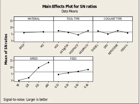
Figure 6: S/N Ratio Response graph of Temperature Figure 7: S/N Ratio Response graph of Surface Roughness
Figure 6 shows the average S/N Ratio of controlled factors affecting the Temperature (smaller is better) and The optimum process parameters are identified as mild steel material at 90 rpm Spindle speed, 0.15 mm/rev feed rate, vegetable oil as lubricant and HSS with Tin coated as Drill tool. Figure 7 shows the average S/N Ratio of controlled factors affecting the Surface roughness (smaller is better) and the optimum process parameters are identified as Mild steel material at 125 rpm Spindle speed, 0.36 mm/rev feed rate, at Dry condition and HSS as drill tool.
MS EN24 15 10 5 0 HSS8 %CO HSS5 %CO
HSS@
TIN HSS VEG OIL KERO SENE DRY DIES EL 450 315 125 90 15 10 5 0 0.36 0.30 0.20 0.15 MATERIAL M e a n o f S N r a ti o s
TOOL TYPE COOLANT TYPE
SPEED FEED
Main Effects Plot for SN ratios Data Means
Signal-to-noise: Larger is better
Figure 8: S/N Ratios Response graph of MRR
Results from Desirability Function Analysis (DFA)
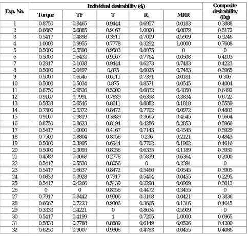
The multiple performances characteristics of the experimental results were evaluated using Desirability Function Analysis (DFA). In this analysis the optimization of multiple performances characteristics the larger-the-better characteristic is applicable to determine the individual desirability values for Material removal rate (MRR) and the smaller-the-better characteristic is applicable to determine the individual desirability values for Temperature, Torque, thrust force and surface roughness. After evaluating the individual desirability of the experimental values then the composite desirability is evaluated according to the formula mentioned and tabulated in Table 3.
Table 3: Evaluated Individual Desirability and Composite Desirability
Exp. No.
Individual desirability (di) Composite
desirability (Dg) Torque TF T Ra MRR
1 0.8750 0.8465 0.9444 0.6957 0.0183 0.3888
2 0.6667 0.6885 0.9167 1.0000 0.0879 0.5172
3 0.5417 0.4898 0.3611 0.7019 0.5909 0.5246
4 1.0000 0.9955 0.7778 0.3292 1.0000 0.7608
5 0.5000 0.5598 0.9583 0.8075 0 0
6 0.5000 0.6433 0.9167 0.7764 0.0508 0.4103
7 0.2917 0.1038 0.9444 0.6273 0.7483 0.4223
8 0.5000 0.0497 0.875 0.6025 0.7483 0.3965
9 0.5000 0.6546 0.6111 0.7391 0.0181 0.306
10 0.5000 0.5034 0.875 0.8571 0.0545 0.4004
11 0.8750 0.9526 0.5000 0.6832 0.4050 0.6492
12 0.9167 0.7991 0.7639 0.6398 0.3834 0.6722
13 0.5833 0.6546 0.8611 0.8882 0.1818 0.5559
14 0.7500 0.5372 0.8472 0.7702 0.0972 0.4803
15 0.9167 0.9819 0.3889 0.3665 0.4545 0.5664
16 0.8750 0.8623 0.8194 0.4286 0.2853 0.5966
17 0.5417 1.0000 0.4167 0.7143 0.4545 0.5929
18 0.7500 0.8804 0.8056 0.236 0.2121 0.4843
19 0.5000 0.3995 0.6944 0.7702 0.1962 0.4616
20 0.5000 0.3093 0.8056 0.6335 0.1189 0.3931
21 0.4583 0.0068 0.2778 0.5839 0.6364 0.2000
22 0.5417 0.5530 0.8056 0 0.2394 0
23 0.5417 0.6637 0.8472 0.5466 0.0545 0.3905
24 0.0833 0.3928 0.7917 0.5404 0.0455 0.2295
25 0.5417 0.4266 0.5139 0.2298 0.0909 0.3013
26 0 0 0.8056 0.4472 0.3455 0
27 0.7917 0.8442 0.9306 0.3168 0.0421 0.3836
28 0.6667 0.7223 0.9306 0.3665 0.1316 0.4645
29 0.3333 0.4221 0 0.8634 0.5909 0
30 0.5417 0.4199 1 0.7205 1.0000 0.6965
31 0.5833 0.7788 0.8889 0.6149 0.0526 0.4200
The individual desirability (di) and composite desirability (Dg) values for each response from experiment using
L32 orthogonal array are tabulated in Table 3. The higher composite desirability value represents that the corresponding
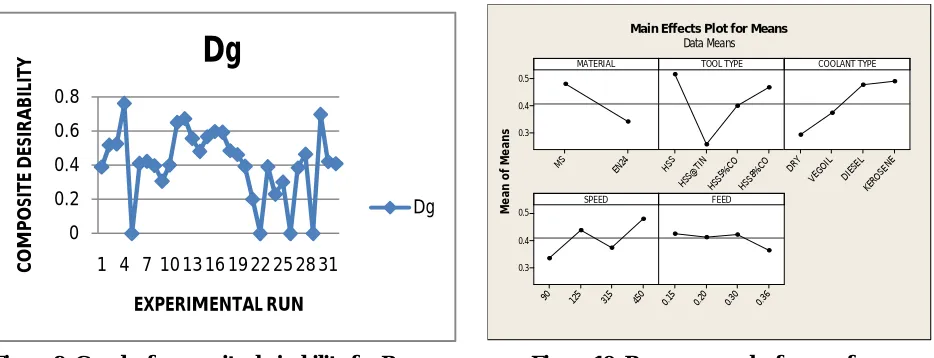
experimental results is closer to the ideally normalized values, graphically showed in Figure-9. In other words optimization of the complicated multiple performance characteristics can be converted into optimization of a single composite desirability.
EN24 MS 0.5 0.4 0.3 HSS 8%C O HSS 5%C O HSS @TI N HS S KERO SEN E DIE SEL VEG OIL DR Y 450 315 125 90 0.5 0.4 0.3 0.36 0.30 0.20 0.15 MATERIAL M e a n o f M e a n s
TOOL TYPE COOLANT TYPE
SPEED FEED
Main Effects Plot for Means
Data Means
Figure 9: Graph of composite desirability for Response Figure 10: Response graph of means for Composite Desirability (Dg)
Effect of process parameters on Composite Desirability (Dg):
Since the experimental design is orthogonal, it is then possible to separate out the effect of each machining parameter on the Mild steel and EN-24 can be studied by using response graph and response table. The mean response values for each level of parameter on composite desirability is calculated and presented in table 4 and graphically shown in figure-10.
Table 4: Response table for the composite desirability Machining
Parameter
Average Composite Desirability
Level 1 Level 2 Level 3 Level 4 Max – Min Material 0.4780 0.3391 - - 0.1389
Tool 0.5154 0.2561 0.3971 0.4655 0.2593
Coolant 0.2931 0.3736 0.4773 0.4902 0.1971
Speed 0.3370 0.4393 0.3752 0.4828 0.1458
Feed 0.4287 0.4156 0.4245 0.3654 0.0633 Total mean of composite desirability=0.2298
Basically, the larger the composite desirability, the better is the multiple performance characteristics. However, relative importance among the machining parameters for the multiple performance characteristics is still needs to be known .so that the optimal combinations of the machining parameter levels can be determined more accurately. From response table and graph, the optimal machining parameters for the combined objective of minimum surface roughness, torque, thrust force, temperature and maximum material removal rate are Material at level 1, tool type at level 1, coolant type at level 4, speed at level 4, and feed rate at level 1 i.e. shown in table 5.
0 0.2 0.4 0.6 0.8
1 4 7 10 13 16 19 22 25 28 31
Table 5: The Values of the optimal process parameters are Exp. No. Speed
(rpm)
Feed
(mm/rev) Material Tool Coolant
1 450 0.15 Mild Steel HSS Kerosene
From Table 5, the mentioned optimal parameter obtained from DESIRABILITY FUNCTION ANALYSIS (DFA) which will give the best results of output responses and minimize the machining cost and increase the production rate. Therefore from table 5, the optimal process parameters from DFA are identified as Mild steel material at 450 rpm Spindle speed, 0.15 mm/rev feed rate, at kerosene as lubricant and HSS as drill tool.
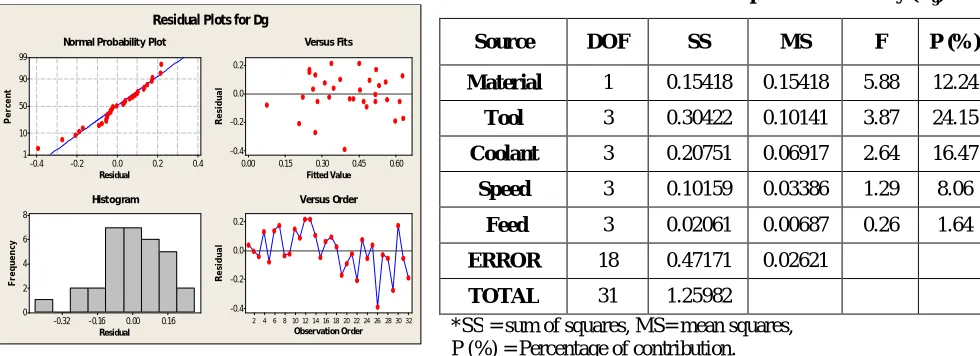
ANOVA for composite desirability
Analysis of variance (ANOVA) is a method of apportioning variability of an output response to various inputs. The purpose of the statistical ANOVA is to investigate which design parameter significantly affects the performance characteristics. This is accomplished by separating the total variability of the composite desirability value, which is measured by sum of the squared deviations from the total mean of the composite desirability value into contributions by each machining parameter and the error. First, the total sum of the squared deviations from the total mean of the composite desirability value can be calculated and showed in table 6.
Table 6: ANOVA for Composite Desirability (Dg)
0.4 0.2 0.0 -0.2 -0.4 99 90 50 10 1 Residual P e r c e n t 0.60 0.45 0.30 0.15 0.00 0.2 0.0 -0.2 -0.4 Fitted Value R e s id u a l 0.16 0.00 -0.16 -0.32 8 6 4 2 0 Residual F r e q u e n c y 32 30 28 26 24 22 20 18 16 14 12 10 8 6 4 2 0.2 0.0 -0.2 -0.4 Observation Order R e s id u a l
Normal Probability Plot Versus Fits
Histogram Versus Order
Residual Plots for Dg
Figure 11: Residual plots for Dg
From the ANOVA Table 6, the Percentage of Contribution values for material type (12.2383), Tool type (24.1479), Coolant type (16.4714), Feed (8.0639), Speed (1.6359), are obtained. It is observed that the Tool type is the most significant machining parameter for affecting the multiple performance characteristics followed by coolant, speed, material type and feed i.e., Tool is the most significant parameter for affecting the multiple performance characteristics. Since this analysis is a parameter based optimization design, from the above values it is clear that Tool is the Major Factor to be selected effectively to get the good multiple performance characteristics.
It can be seen in Figure 11, that all the points on the normal probability plot lies close to the straight line (mean line). This implies that the data are fairly normal and a little deviation from the normality is observed. This shows the effectiveness of the developed model. It is noticed that the residuals fall on a straight line, which implies that errors are normally distribution.
Source DOF SS MS F P (%) Material 1 0.15418 0.15418 5.88 12.24
Tool 3 0.30422 0.10141 3.87 24.15
Coolant 3 0.20751 0.06917 2.64 16.47
Speed 3 0.10159 0.03386 1.29 8.06
Feed 3 0.02061 0.00687 0.26 1.64
ERROR 18 0.47171 0.02621
TOTAL 31 1.25982
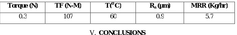
Confirmation Experiment Results
Confirmation experiments are conducted as per the optimal level of the machining parameter for testing drilling characteristics of MS and results are recorded (Table 7). The performance characteristics such as Torque, Thrust force, Temperature, Surface roughness and maximize material removal rate (MRR) are improved together by using above proposed method. It can be observed from confirmatory test results showed in table 7.
Table 7: Confirmation test results
Torque (N) TF (N-M) T(0 C) Ra (µm) MRR (Kg/hr)
0.3 107 60 0.9 5.7
V. CONCLUSIONS
Based on the investigation the following conclusions were drawn from the present study. Taguchi method has been successfully applied in determining optimum conditions for minimum Torque, Thrust force, Temperature, Surface roughness and maximize material removal rate (MRR). The optimum parameter combination for Torque is Mild steel material at 450 rpm Spindle speed, 0.15 mm/rev feed rate, kerosene as lubricant and HSS as Drill tool. The optimum parameter combination forThrust force is 450 rpm Spindle speed, 0.15 mm/rev feed rate, Diesel as lubricant and HSS as Drill tool. The optimum parameter combination for Temperatureis90 rpm Spindle speed, 0.15 mm/rev feed rate, vegetable oil as lubricant and HSS with Tin coated as Drill tool. The optimum parameter combination for surface roughness is (Ra) was obtained at Mild steel material at 125 rpm Spindle speed, 0.36 mm/rev feed rate, at Dry condition and HSS as drill tool and The optimum parameter combination for material removal rate (MRR) was obtained at 450 rpm Spindle speed, 0.36 mm/rev feed rate, at kerosene as lubricant and HSS with 8% cobalt as Drill Tool. From Desirability Function Analysis (DFA) the optimal machining parameters for the combined objective of minimum surface roughness, torque, thrust force, temperature and maximum material removal rate are Material at level 1, tool type at level 1, coolant type at level 4, speed at level 4, feed rate at level 1 i.e. spindle speed 450(rpm), feed rate 0.15 (mm/min), at kerosene as lubricant and HSS as drill tool on Mild steel material. From ANOVA, It is observed that the Tool type is the most significant machining parameter for affecting the multiple performance characteristics followed by coolant, speed, material type and feed i.e., Tool is the most significant parameter for affecting the multiple performance characteristics.
The performance characteristics such as Torque, Thrust force, Temperature, Surface roughness and maximize material removal rate (MRR) are improved together by using above proposed method. It can be observed from confirmatory test results.
REFERENCES
[1] Anderson Mark J. and Whitcomb Patrick J, ― “DOE Simplified, Practical Tools for Effective Experimentation,” 2nd edition. United States of America: Edward Brothers, 2000.
[2] Gurpreet Singh, Sehijpal Singh, Manjot Singh, Ajay Kumar - experimental investigations of vegetable & mineral oil performance machining of EN-31 steel with minimum quantity lubrication, IJRET, volume 2, Issue 06, June 2013.
[3] Professor Toshiaki WAKABAYASHI – The role of Tribology in environmentally friendly MQL Machining, ITEKT, edition no. 1007E, 2010 [4] Professor S.C.Brose, K.S.Bansode – MQL applications in reaming – A review, IJIRSET, Volume 3, special issue 4, April 2014
[5] Adikesavulu, Sreenivasulu.Bathina, Sreenivasulu.Bezavada, 2014 “Optimization of process parameters in drilling of EN31 steel using Taguchi method”, IJIERT, Volume 1, issue 1, nov-2014
[6] Kunal Sharma, Mr.Abhishek jatav, “Optimization of machining parameters in drilling of stainless steel”, IJSRET, Volume 4,issue 8, aug-2015
[7] G.Vijaya kumar, P.venkataramaiah “selection of optimal parameters in drilling of aluminium metal matrix composites using desirable-fuzzy approach”, ISSN: 2320-2491, Vol.2, No.5, Aug-Sep 2013
[8] Pantawane.P.D, Ahuja.B.B., “experimental investigations and multi-objective optimization of friction drilling on AISI 1015”, International journal of applied engineering research, Dindigul, vol.2, no.2, 2011
[9] Md.anayet U.Patwari, S.M.Tawfiq ullah, Ragib Ishraq khan, Md.Mahfujur Rahman – “prediction and optimization of surface roughness by coupled statistical and desirability analysis in drilling of mild steel”, ANNALS of faculty engineering hunedoara, tome IX, 2013