More powerful tests from confidence interval P values

More Powerful Tests from Confidence Interval

P

Values

Roger L. Berger

Department of Statistics

North Carolina State University

Raleigh, NC 27695-8203

December 20, 1995

Institute of Statistics Mimeo Series No. 2281

Abstract

In this article, the problem of comparing two independent binomial populations is considered. It is shown that the test based on the confidence intervalpvalue of Berger

and Boos (1994) often is uniformly more powerful than the standard unconditional test. This test also requires less computational time.

KEY WORDS: Binomial, Confidence interval, Contingency table, Homogeneity test, Independence,P value, 22 table.

1

INTRODUCTION

The problem of comparing two binomial proportions has been considered for many years. The most commonly used test is Fisher’s Exact Test (Fisher, 1935), a conditional test. Barnard(1945, 1947) proposed an unconditional test for this problem. Although uncon-ditional tests are usually more powerful than conuncon-ditional tests, they are computationally much more complex. But recent advances in computing have made unconditional tests practical, and they are beginning to appear in statistical software packages such as

StatXact 3 for Windows. In this article it is shown that unconditional tests based on the confidence interval

p

value of Berger and Boos (1994) are often uniformly more powerful than the standard unconditional tests.

and the success probability is

p

1. The sample size for

Y

is

n

and the success probability

is

p

2. The binomial probability mass function of

X

will be denoted by

b

(

x

;

m;p

1)=

C

m

x

p

x

1(1?

p

1)

m

?

x

; x

=0

;:::;m;

where

C

_x

m

=

m

!

=x

!

=

(

m

?

x

)! is the binomial coefficient. Similarly,

b

(

y

;

n;p

2)will denote the

binomial probability mass function of

Y

. The sample space of(

X;Y

) will be denoted by

X =f0

;:::;m

gf0

;:::;n

g. X contains(

m

+1)(

n

+1) points.

This kind of data is often displayed in a 22 contingency table as follows.

yes no

Population 1

X

m

?

X

m

Population 2

Y

n

?

Y

n

R

=

X

+

Y t

?

R t

=

m

+

n

In this table, upper case letters denote random variables and lower case letters denote known constants fixed by the sampling scheme. So,

t

is the total sample size, and

R

is the observed number of successes. Conditional inference is based on the conditional distribution of

X

and

Y

, given the observed marginal

R

=

r

=

x

+

y

.

Consider the problem of testing

H

o

:

p

1 =

p

2 versus

H

a

:

p

1

< p

2

:

(1)

Exact tests for this problem will be considered. The sizes of the tests are computed using the exact binomial distributions, not normal or chi-squared approximations. The standard Neyman-Pearson paradigm of restricting consideration to level-

tests and then comparing the powers of these tests will be followed. For a specified error probability

, all tests considered are level-

tests. Tests that are liberal, that sometimes have type-I error probabilities that are greater than

, are not considered. However, the tests do not have sizes exactly equal to the specified

. Because of the discrete nature of this data, equality can (usually) be achieved only with a randomized test. Because randomized tests are not of any practical interest, this article considers only nonrandomized tests.

this debate. The purpose of this article is not to continue this debate. Rather, suffice it to say that this article is relevant to those situations in which the unconditional analysis is appropriate.

2

USUAL UNCONDITIONAL TEST

Barnard (1945, 1947) first proposed an unconditional test for this problem. Because of the computational difficulty of unconditional tests, they were not widely used until recently. NOw, computing technology makes the use of unconditional tests feasible.

A commonly used unconditional test is the the

Z

test proposed by Suissa and Shuster (1985) and Haber (1986). Define the

Z

-pooled statistic (score statistic) as

Z

(

x;y

)=

^

p

2?

p

^1 r

^

p

(1?

p

^)

1

m

+

1

n

;

where

p

^1 =

x=m

,

p

^2 =

y=n

, and

p

^= (

x

+

y

)

=

(

m

+

n

), the pooled estimate of

p

1 =

p

2 =

p

under

H

o

. Then, the

p

value for testing (1), using the test statistic

Z

, is

p

Z

(

x;y

)= sup

0

p

1

P

p

?

Z

(

X;Y

)

Z

(

x;y

)

= sup

0

p

1

X

(

a;b

)2

R

Z

(

x;y

)

b

(

a

;

m;p

)

b

(

b

;

n;p

)

;

(2)

where

R

Z

(

x;y

) = f(

a;b

) : (

a;b

) 2 X and

Z

(

a;b

)

Z

(

x;y

)g. The

p

value is the maximum

probability under

H

o

of observing a value of the test statistic equal to or more extreme than the value observed in the data. This is a standard definition of a

p

value, such as is found in Bickel and Doksum (1977, Section 5.2.B). Rejection of

H

o

if and only if

p

Z

defines a level-

test of (1). The calculation of the supremum in (2) must be

done numerically. Typically there is no simple formula for this value. This numeric maximization has been the cause of the computational difficulty of unconditional tests.

3

CONFIDENCE INTERVAL P VALUE

Berger and Boos (1994) proposed a new method of computing a

p

value. In the problem of comparing two binomial proportions, if

H

o

is true,

p

=

p

1=

p

2 is a nuisance parameter.

Let

C

(

x;y

)denote a 100(1?

)% confidence interval for

p

calculated from the data(

x;y

)

and Pearson (1934) interval based on

X

+

Y

, a binomial(

m

+

n;p

) random variable if

p

1 =

p

2 =

p

. This interval is easily computed from the formula

a

a

+(

b

?

a

+1)

F

2(

b

?

a

+1)

;

2

a;=

2

p

(

a

+1)

F

2(

a

+1)

;

2(

b

?

a

)

;=

2

b

?

a

+(

a

+1)

F

2(

a

+1)

;

2(

b

?

a

)

;=

2

(3)

where

a

=

x

+

y

,

b

=

m

+

n

, and

F

;;=

2is the upper 100(

=

2)percentile of an

F

distribution

with

and

degrees of freedom.

The confidence interval

p

value, based on the statistic

Z

is defined by

p

C

(

x;y

) = sup

p

2

C

(

x;y

)

P

p

?

Z

(

X;Y

)

Z

(

x;y

)

+

= 0 @ sup

p

2

C

(

x;y

)

X

(

a;b

)2

R

Z

(

x;y

)

b

(

a

;

m;p

)

b

(

b

;

n;p

) 1 A

+

;

where

R

Z

(

x;y

) is the same as in the definition of

p

Z

.

p

C

differs from

p

Z

in that the

supremum is taken over the confidence interval

C

(

x;y

) rather than over the whole

range 0

p

1, and the error probability

is added to the supremum. If

= 0,

p

C

is the same as

p

Z

. Berger and Boos (1994) showed that this modification of the usual definition of a

p

value yields a valid

p

value. That is, the test that rejects

H

o

if and only if

p

C

(

X;Y

)

is an unconditional level-

test. The error probability is specified by the

experimenter. Different values of

yield different

p

values and tests. In this article,

=

:

001 is used (as suggested by Berger and Boos).

Berger and Boos proposed the confidence interval based

p

value for two reasons. The first is computational. In both

p

Z

and

p

C

, the function to be maximized is the same. The maximization over the smaller set,

C

, can be much simpler. The second is statistical. Having observed the data, we should be able to estimate

p

and should not need to consider values of

p

that are completely unsupported by the data. In

p

C

, only those “plausible” values that are in the confidence interval are considered.

This article points out that the confidence interval

p

value can have a third advan-tage. It can produce tests with higher power than the usual

p

value. And, remember, this is achieved with less computational effort.

4

EXAMPLE

An enumeration of

p

Z

(

x;y

) for all the sample points in X shows that the point

(

x;y

) = (23

;

15) has the largest value of

p

Z

(

x;y

) that is less than or equal to

=

:

10.

Z

(23

;

15)=1

:

454 and

p

Z

(23

;

15)=

:

0823. The sample point with the next smaller value

of

Z

is (

x;y

) = (0

;

1) with

Z

(0

;

1) = 1

:

407 and

p

Z

(0

;

1) =

:

1548. So (0

;

1), or any other

sample point with a smaller value of

Z

, is not in the level

=

:

10 rejection region based

on

p

Z

.

Let the p value functionfor a sample point(

x;y

)be defined by

Z

(

p

;

x;y

)=

X

(

a;b

)2

R

Z

(

x;y

)

b

(

a

;

m;p

)

b

(

b

;

n;p

)

:

(4)

The

p

value function is the function that is maximized in calculating

p

Z

and

p

C

. In Figure 1,

Z

(

p

; 23

;

15) (solid line) and

Z

(

p

; 0

;

1) (long dashed line) are shown.

Z

(

p

; 23

;

15)

<

:

10 =

for all values of

p

. Its maximum value is

p

Z

(23

;

15) =

:

0823 which occurs at

p

=

:

524. Because

p

Z

(23

;

15) is the largest

p

value not exceeding

=

:

10, .0823 is also

the actual size of the level

=

:

10 test constructed using

p

Z

. The addition of the single

sample point (0

;

1) to the rejection region causes a large spike to appear in

Z

(

p

; 0

;

1).

The maximum of

Z

(

p

; 0

;

1)is

p

Z

(0

;

1)=

:

1548 which occurs at

p

=

:

026. It is not unusual

for the addition of a single sample point with

x

+

y

close to 0 or

m

+

n

to create a spike

like this.

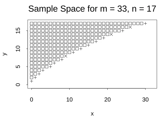
In Figure 2, the sample points in X with

p

Z

(

x;y

)

:

10 are marked by 2’s. These

are the elements of the level

=

:

10 rejection region defined by

p

Z

. Because the actual

size of this test is only .0823, not too close to

=

:

10, it seems possible that some more

points, some of the points marked by ’s and +’s, for example, might be added to this

rejection region and the resulting test could still be level

=

:

10. The points marked

by+’s and ’s are the points that satisfy the “convexity” property of Barnard (1947). It

would take a great deal of computation to try each point individually, then try pairs or triples of points, to determine points that could be added. But the use of the confidence interval

p

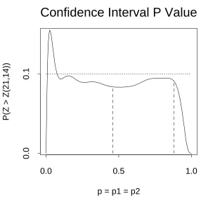
value easily identifies some points that can be added.

Consider(

x;y

)=(21

;

14)with

Z

(21

;

14)=1

:

368. There are four sample points with

Z

(21

;

14)

< Z

(

x;y

)

< Z

(23

;

15), namely,

Z

(0

;

1) = 1

:

407,

Z

(26

;

16) = 1

:

401,

Z

(9

;

8) =

1

:

399, and

Z

(3

;

4)=1

:

394. The

p

value function

Z

(

p

; 21

;

14)is shown in Figure 3. The

maximum of this function, .1549, is greater than .10 because

Z

(0

;

1)

> Z

(21

;

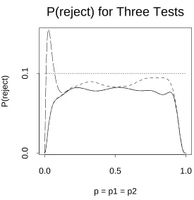
14). But

calcu-P(reject) for Three Tests

p = p1 = p2

P(reject)

0.0

0.5

1.0

0.0

0.1

Figure 1:

P

(reject) for three rejection regions defined by f

Z

Z

(23

;

15)g (solid line),

f

Z

Z

(0

;

1)g(long dashes), and f

p

C

:

10g(short dashes).

lated from the data (

x;y

) = (21

;

14). Using (3), this confidence interval is [

:

459

;:

881].

These confidence limits are shown in Figure 3. The maximum of

Z

(

p

; 21

;

14) over

this interval is .0946 and this maximum occurs at

p

=

:

830. Therefore,

p

C

(21

;

14) =

:

0946+

=

:

0946+

:

0010 =

:

0956. Because,

p

C

(21

;

14)

:

10, (21

;

14) is in the level

=

:

10 rejection region defined by

p

C

. In addition, two other points are in the level

=

:

10 rejection region defined by

p

C

. These are (26

;

16) with

p

C

(26

;

16) =

:

0949 and

(9

;

8) with

p

C

(9

;

8)=

:

0906. These three added points are the points marked with’s in

Figure 2.

Because the rejection region of the level

=

:

10 test defined by

p

Z

is a proper

subset of the rejection region of the level

=

:

10 test defined by

p

C

, the test defined by

p

C

is uniformly more powerful.

The probability of the level

=

:

10 rejection region defined by

p

C

, that is, the

Sample Space for m = 33, n = 17

x

y

0

10

20

30

0

5

10

15

Figure 2: 2’s are sample points in level

=

:

10 test defined by

p

Z

. +’s and ’s are

sample points that might be added. ’s are three points added by test defined by

p

C

.

is graphed in Figure 1 with a short dashed line. This probability is less than .10 for all values of

p

, because this is a level

=

:

10 test. But this probability is much closer to

.10 than the probability of the rejection region for the Suissa and Shuster test defined by

p

Z

. The actual size of the

p

C

test is .0946, the maximum of this function.

5

CONSISTENCY OF IMPROVEMENT

In the previous section it was shown that, for

=

:

10 and (

m;n

) = (33

;

17), the

con-fidence interval

p

value defines a uniformly more powerful, level-

test than the usual unconditional

p

value. The question arises as to the generality of this phenomenon. To investigate this we enumerated the level-

rejection regions defined by

p

Z

and

p

C

for

=

:

10, .05 and .01 for each of nine different sample sizes, (

m;n

) = (10

;

10), (13

;

7),

(16

;

4), (25

;

25), (33

;

17), (40

;

10), (50

;

50), (65

;

35), and (80

;

20). These sample sizes

Confidence Interval P Value

p = p1 = p2

P(Z > Z(21,14))

0.0

0.5

1.0

0.0

0.1

Figure 3: Confidence interval

p

value

p

C

(21

;

14) =

:

0956 is the maximum of

Z

(

p

; 21

;

14)+

:

001 over the 99.9% confidence interval [

:

459

;:

881].

Z

(

p

; 21

;

14) is the

function shown and the confidence interval is marked by vertical lines.

In 15 out of the 27 cases, the rejection region defined by

p

Z

is a proper subset of the rejection region defined by

p

C

. So the confidence interval

p

value defines a uniformly more powerful, level-

test. In another 9 out of the 27 cases, the rejection regions defined by the two

p

values are exactly the same. In one case,

=

:

01 and (

m;n

) = (50

;

50),

neither rejection region contained the other and the power functions of the two tests crossed. In the remaining two cases.

=

:

01 and (

m;n

) = (13

;

7) and (25

;

25), the

rejection region defined by

p

C

is a proper subset of the rejection region defined by

p

Z

, and

p

Z

defines a uniformly more powerful test. The power functions for the nine tests with

=

:

10 are described more fully by Berger (1994).

all cases, the computation required for

p

C

is less than that required for

p

Z

.

The reason that the rejection region defined by

p

C

usually contains the rejection region defined by

p

Z

is the following fact. If there is no sample point in X such that

?

< p

Z

(

x;y

)

, then every sample point with

p

Z

(

x;y

)

also satisfies

p

C

(

x;y

)

.

That is, every sample point in the level-

rejection region defined by

p

Z

is also in the level-

rejection region defined by

p

C

. This fact is true because, if

p

Z

(

x;y

)

, then

p

Z

(

x;y

)

?

, and, hence,

p

C

(

x;y

) = sup

p

2

C

(

x;y

)

P

p

?

Z

(

X;Y

)

Z

(

x;y

)

+

sup

0

p

1

P

p

?

Z

(

X;Y

)

Z

(

x;y

)

+

=

p

Z

(

x;y

)+

(

?

)+

=

:

When

is small compared to

, as with the

=

:

001 recommended by Berger and Boos

(1994) that is used in this article, it often happens that there is no sample point with

?

< p

Z

(

x;y

)

. In such cases the test defined by

p

C

will be at least as powerful

as the test defined by

p

Z

. Note, this property applies in general to confidence interval

p

values, not just this problem and this test statistic

Z

.

6

OTHER TEST STATISTICS

Other statistics besides

Z

(

x;y

), such as the likelihood ratio test statistic and

p

^2 ?

p

^1,

can be used to test (1). Santner and Duffy (1989, Exercises 5.11 and 5.12), Haber (1987), and Mart´in and Silva (1994) list several possible statistics. The experience with

Z

suggests that if another statistic is used, the confidence interval

p

value might provide improved power over the usual unconditional

p

value.

The power comparisons of Haber (1987) and Mart´in and Silva (1994) suggest that the two statistics

Z

(

x;y

) and

B

(

x;y

)=

min(

n;x

+

y

) X

a

=

y

C

_x

m

+

y

?

a

C

na

C

_tx

+

y

produce tests with the highest power. The statistic

B

(

x;y

)was first proposed by Boschloo

Fisher’s Exact Test (Fisher, 1935). Here,

B

(

x;y

) is not used as a

p

value, but, rather, as

a statistic to order the sample points. Small values of

B

(

x;y

)give evidence for

H

a

so the

unconditional

p

value based on

B

(

x;y

)is

p

B

(

x;y

)= sup

0

p

1

P

p

?

B

(

X;Y

)

B

(

x;y

)

= sup

0

p

1

X

(

a;b

)2

R

B

(

x;y

)

b

(

a

;

m;p

)

b

(

b

;

n;p

)

;

where

R

B

(

x;y

)=f(

a;b

): (

a;b

)2X and

B

(

a;b

)

B

(

x;y

)g. The confidence interval

p

value

based on

B

is defined as in (4), namely,

p

CB

(

x;y

)= 0 @ sup

p

2

C

(

x;y

)

X

(

a;b

)2

R

B

(

x;y

)

b

(

a

;

m;p

)

b

(

b

;

n;p

) 1 A

+

:

Berger (1994) found that the

p

value function

B

(

p

;

x;y

) tends to be flatter than

Z

(

p

;

x;y

), especially for unequal sample sizes. This agrees with Mart´in and Silva’s

(1994) finding that the unconditional test based on

B

usually has higher power than the test based on

Z

, especially when

m

6=

n

. So there is less room for improvement of

Boschloo’s test. But, Berger (1994) found that, as with

p

Z

and

p

C

, the confidence interval

p

value,

p

CB

, usually defined a test that was the same or uniformly more powerful than the test defined by

p

B

.

In comparing the tests based on the two confidence interval

p

values, Berger (1994) did not find a clear preference. Usually the power functions of these two tests crossed with one test having higher power for some parameter values and the other having higher power for other parameter values. Usually, the power function defined by

p

CB

was higher on a majority of the parameter space.

In their power comparison of tests for (1), Mart´in and Silva (1994) considered two computationally intensive tests they called

M

and

M

0

.

M

is the test proposed by Barnard (1945, 1947), and

M

0

is a simplified version of

M

. Both methods involve construction of a rejection region by adding one sample point at a time, with a good deal of computation required to determine which point is added next. Mart´in and Silva report that

M

0

and

M

require about 10 and 85 times the computation time required by

p

Z

or

p

B

, respectively. But,

M

and

M

0

do provide some improvement in power. In this article it has been shown that confidence interval

p

values provide an improvement in power over

p

Z

or

p

B

, but with

lesscomputation. It remains to be determined if the improvement in power provided by

p

C

or

p

CB

is comparable to the improvement provided by

M

0

7

CONCLUSIONS

Confidence interval

p

values can improve the power of standard unconditional tests for comparing two binomial populations. They also require less computational effort. Thus, they offer a promising new method for the analysis of 22 tables.

Similar, but less extensive, comparisons have have been made for two-sided tests. The results are qualitatively the same. The confidence interval

p

value often defines a more powerful test than the standard

p

value.

XUN2X2 is a FORTRAN program that will compute the standard and confidence interval

p

values discussed in this article. The program will also perform uncondi-tional tests for multinomial, rather than two independent binomials, 2 2 tables.

XUN2X2 may be obtained by sending the one line message “get exact from general” to [email protected].

References

Barnard, G. A. (1945). A new test for 22 tables. Nature, 156:177.

Barnard, G. A. (1947). Significance tests for 22 tables. Biometrika, 34:123–138.

Berger, R. L. (1994). Power comparison of exact unconditional tests for comparing two binomial proportions. Technical Report 2266, North Carolina State University Statis-tics Department.

Berger, R. L. and Boos, D. D. (1994).

P

values maximized over a confidence set for the nuisance parameter. Journal of the American Statistical Association, 89:1012–1016.

Bickel, P. J. and Doksum, K. A. (1977).Mathematical Statistics: Basic Ideas and Selected Topics. Holden-Day, San Francisco.

Boschloo, R. D. (1970). Raised conditional level of significance for the 22-table when

testing the equality of two probabilities. Statistica Neerlandica, 24:1–35.

Fisher, R. A. (1935). The logic of inductive inferences. Journal of the Royal Statistical Society, Series A, 98:39–54.

Greenland, S. (1991). On the logical justification of conditional tests for two-by-two contingency tables. American Statistician, 45:248–251.

Haber, M. (1986). An exact unconditional test for the 22 comparative trial.Psychological

Bulletin, 99:129–132.

Haber, M. (1987). A comparison of some conditional and unconditional exact tests for 22 contingency tables. Communications in Statistics–Simulation and Computation,

16:999–1013.

Little, R. J. A. (1989). Testing the equality of two independent binomial proportions.

American Statistician, 43:283–288.

Mart´in Andr´es, A. and Silva Mato, A. (1994). Choosing the optimal unconditioned test for comparing two independent proportions.Computational Statistics and Data Anal-ysis, 17:555–574.

McDonald, L. L., Davis, B. M., and Milliken, G. A. (1977). A nonrandomized uncondi-tional test for comparing two proportions in 22 contingency tables. Technometrics,

19:145–157.

Mehta, C. and Patel, N. (1995). StatXact 3 for Windows: User Guide. Cytel Software, Cambridge, MA.

Santner, T. J. and Duffy, D. E. (1989). The Statistical Analysis of Discrete Data. Springer-Verlag, New York.

Suissa, S. and Shuster, J. J. (1985). Exact unconditional sample sizes for the 22