Modified Milne Simpson Method for Solving Differential Equations

(1)

ISSN(Online): 2319-8753 ISSN (Print): 2347-6710

I

nternational

J

ournal of

I

nnovative

R

esearch in

S

cience,

E

ngineering and

T

echnology

(A High Impact Factor & UGC Approved Journal)

Website: www.ijirset.com

Vol. 6, Issue 8, August 2017

Modified Milne Simpson Method for Solving

Differential Equations

R. K. Devkate 1, R. M. Dhaigude 2

Research Student, Department of Mathematics, Dr. Babasaheb Ambedkar Marathwada University, Aurangabad,

Maharashtra, India1

Head and Associate Professors, P. G. Department of Mathematics, Government Vidarbha Institute of Science and

Humanities, Amravati, Maharashtra, India2

ABSTRACT: In the present paper, modified Milne Simpson method have been developed for solving ordinary differential equations. We apply Daftardar-Gejji and Jafari iterative method on implicit Milne Simpson method to derive the proposed method. The efficiency and error of this method is tested through various types of numerical test problems. It is observed that the proposed method gives better solution as comparative to other methods.

KEYWORDS: Daftardar-Gejji and Jafari method (DJM), Delay differential equations, Milne Simpson method, Numerical solution.

I. INTRODUCTION

In the real life phenomena for the study of many branches of science, engineering, technology, economics and biological field’s ordinary differential equations (ODEs) play a very important role. Delay differential equations (DDEs) frequently occur in the class of dynamical systems. They are naturally arising in electro dynamics, population dynamics, chemical kinetics, physiology, communication network [1], [2], [3], [10], [11], [17]. To obtain the analytical solution of DDEs are very difficult than ODEs. For such types of problems numerical techniques plays a crucial role to finding the solution. During the past thirty years, implemented the numerical solution of DDEs based on the extension or modification of traditional ODEs numerical methods such as Modified power series method [13], Nakashima's two stages fourth order Pseudo-Runge-Kutta method [12], A Legendre-Gauss collocation method [16], Variational iteration method [7], Parallel block method [8], Two-point predictor-corrector block method [9], An efficient unified approach [18]. Recently, Sukale and Daftardar-Gejji [15] developed modified trapezoidal rule and Adams-Moultan method by using the new iterative method for solving DDEs. In this paper, we improved a numerical method by using the power of Daftardar-Gejji and Jafari method (DJM) on Milne Simpson method for solving ODEs (with and without delay terms). Further, we have solved different types of numerical test problems by using software package Maple-8. It shows that the results are matching with exact solutions and more accurate than existing methods. We have organized the paper as follows.

In section 2, we discussed the some preliminaries. The DJM is presented briefly in section 3. Modified Milne Simpson method using DJM is presented in section 4. Numerical test problems show that efficiency of the newly proposed method comparative to other methods in section 5 and finally conclusions are summarized.

II. PRELIMINARY

In this section, we discussed some preliminary concept [2], [5], [6], [14]. Consider the initial value problem (IVP) for delay differential equations

(2)

I

nternational

J

ournal of

I

nnovative

R

esearch in

S

cience,

E

ngineering and

T

echnology

( ) = ( ) , − ≤ ≤0, (2.1)

where is called delay (or lags), which is always non-negative. Delay ( ) may be just constant (the constant delay case) or function of t, = ( ) (the variable or time dependent delay case) or function of and itself, = ( , ( ))

(the state dependent delay case).

The term ( − ) in equation (2.1) is called delay term and the approximation of the delay term is denoted by [15]. Integrating equation (2.1) from the grid point t to t on both sides, we get

= + , ( ), ( − ) (2.2)

Milne Simpson Method:

To finding the solution of initial value problem for DDEs (2.1), the predictor and corrector formulae are given by

= +4ℎ

3 (2 − + 2 ),

and

= +ℎ

3 −4 + ,

which method is known as Milne Simpson predictor-corrector method.

III.DAFTARDAR-GEJJIANDJAFARIMETHOD(DJM)

In the present section, we describe a new iterative method introduced by Daftardar-Gejji and Jafari (DJM) [4] for solving linear and nonlinear functional equation of the form

= + ( ), (3.1)

where f is a known function and N is a nonlinear operator. It is assumed that DJM solution of equation (3.1) in the form of series

= . ∞

(3.2)

In this method, non linear operator N in equation (3.1) is decomposed by DJM as follows:

( ) = . ∞ = ( ) + − ∞ = ∞

, (3.3)

where = ( ) and = ∑ − ∑ , ≥1.

(3)

I

nternational

J

ournal of

I

nnovative

R

esearch in

S

cience,

E

ngineering and

T

echnology

= +

∞ ∞

. (3.4)

Now we define, the DJM series terms from the equation (3.4) as bellow:

=

= ( )

= ( + +⋯ )− ( + +⋯ ), = 1,2, …

Thus kth term approximate solution is given by

= , (3.5)

for suitable integer k.

IV.MODIFIEDMILNESIMPSONMETHOD

In this section, we developed modification of Milne Simpson method by employing Daftardar-Gejji and Jafari method. The value of definite integral on right hand side in the equation (2.2) is approximated by Milne Simpson implicit method is

= +ℎ

3 ( , , ) + 4 ( , , ) + ( , , ) (4.1)

= 3, 4, … , −1,

where ℎ= − and = + ℎ, = 0, 1, 2, ….

Now, we can write equation (4.1) is of the form = + ( )

where

=

= = +4ℎ

3 ( , , ) +

ℎ

3 ( , , ) (4.2)

( ) =ℎ

3 ( , , ).

Now, let us apply DJM on the equation (4.1) to get 4-term solution as

= + + +

= + ( ) + ( + )− ( ) + ( + + )− ( + )

= + + ( ) + ( + )− ( )

= + + + ( ) .

Therefore, equation (4.1) becomes

(4)

I

nternational

J

ournal of

I

nnovative

R

esearch in

S

cience,

E

ngineering and

T

echnology

= +ℎ

3 , +

ℎ

3 , +

ℎ

3 , , , , , (4.3)

where y given by the equation (4.2) is called as predictor and y given by the equation (4.3) is called as corrector and y

denotes the approximate value of the solution at the node t . In this way, we get the new numerical method named as a modified Milne Simpson method given by the equations (4.2) and (4.3) for solving DDEs.

4.1 Modified Milne Simpson method for ODEs

The modification of the Milne Simpson method presented in “modified Milne Simpson method” section can be reduced to solve ODEs by substituting = 0 in equation (4.3). Thus we have solving the IVP

′₌ _{, ( ) ,}

(0) = ,

the following modified Milne Simpson method by applying 4- term DJM as

= +ℎ

3 , +

ℎ

3 , +

ℎ

3 , ,

where

= +4ℎ

3 ( , ) +

ℎ

3 ( , )

V. NUMERICALTESTPROBLEMS

In this section, we illustrate some numerical problems which are solved by using mathematical software Maple-8.

Problem (5.1): Consider the following logistic delay differential equation [11]

′_{( ) =} _{( )(1}₋ ₍ ₋_1)),

(5)

I

nternational

J

ournal of

I

nnovative

R

esearch in

S

cience,

E

ngineering and

T

echnology

(6)

I

nternational

J

ournal of

I

nnovative

R

esearch in

S

cience,

E

ngineering and

T

echnology

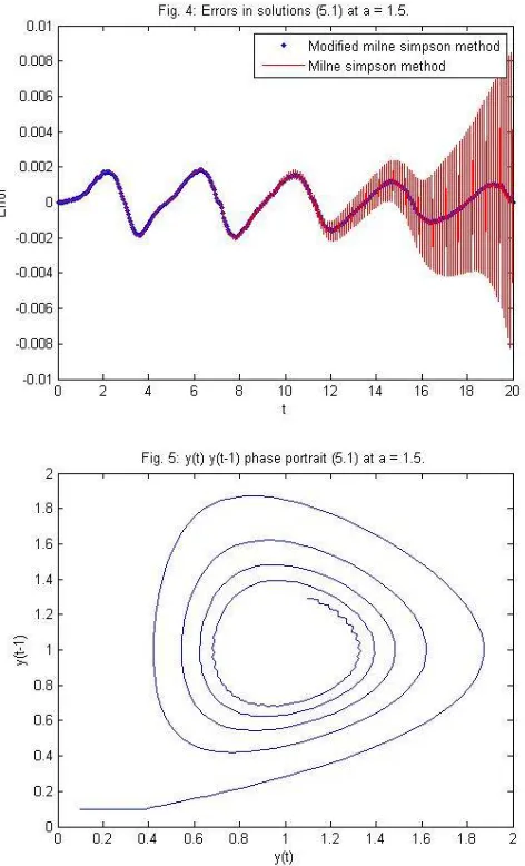
We compare the graphs of solutions of problem (5.1) obtained by modified Milne Simpson method (red), Milne Simpson method (green) and exact solutions (method of steps) (blue) for values of the parameter = 0.3 and = 1.5

in figure (1) and (3) respectively. It is observed that ours solutions are good agreement with exact solutions. Errors in solution of (5.1) obtained by modified Milne Simpson method (red) and Milne Simpson method (blue) compared in figure (2) at = 0.3 and modified Milne Simpson method (blue) and Milne Simpson method (red) compared in figure (4) at = 1.5. It shows that error in modified Milne Simpson method is less than in Milne Simpson method. Hence it can be concluded that ours method is more accurate than Milne Simpson method. Solution of problem (5.1) for a=1.5 in the phase plane is depicted in figure (5).

Problem (5.2): Consider the following delay differential equation [2]

′_{( ) =} 0.2 ( − )

1 + ( − ) −

( ) 10,

(7)

I

nternational

J

ournal of

I

nnovative

R

esearch in

S

cience,

E

ngineering and

T

echnology

(8)

I

nternational

J

ournal of

I

nnovative

R

esearch in

S

cience,

E

ngineering and

T

echnology

(9)

I

nternational

J

ournal of

I

nnovative

R

esearch in

S

cience,

E

ngineering and

T

echnology

In figure (6) and (9), we compare the solutions of problem (5.2) obtained by modified Milne Simpson method (red) and exact solutions (method of steps) (blue) for the values of the parameter = 15 and = 20 respectively. It is observed that the numerical solutions are good agreement with exact solutions. The error in the numerical solutions is plotted in the figure (7) and (10) for = 15 and = 20 respectively and phase portraits of solutions (5.2) for = 15 and = 20

is depicted in the figure (8) and (11) respectively.

VI. CONCLUSION

(10)

I

nternational

J

ournal of

I

nnovative

R

esearch in

S

cience,

E

ngineering and

T

echnology

REFERENCES

[1] C. T. H. Baker, “Retarded differential equations,” Journal of computational and applied mathematics, vol. 125, pp. 309-325, 2000. [2] A. Bellen and M. Zennaro, Numerical methods for delay differential equations, Oxford university press, Oxford, 2003.

[3] S. Bhalekar and V. Daftardar-Gejji, “Fractional ordered liu system with time delay,” Communications in nonlinear science and numerical simulation, vol. 15, no. 8, pp. 2178-2191, 2010.

[4] V. Daftardar-Gejji and H. Jafari, “An iterative method for solving nonlinear functional equations,” Journal of Mathematical Analysis and Applications, vol. 316, pp. 753-763, 2006.

[5] R. M. Dhaigude and R. K. Devkate, “Solution of first order initial value problem by sixth order predictor corrector method,” Global journal of pure and applied mathematics, vol. 13, no. 6, pp. 2277-2290, 2017.

[6] R. V. Dukkipati, Numerical methods, New age international (p) limited, New Delhi, 2010.

[7] J. He, “Variational iteration method for delay differential equations,” Communications in nonlinear science and numerical simulation, vol. 2, no. 4, pp. 235-236, 1997.

[8] F. Ishak, “Parallel block method for solving delay differential equations,” International mathematical forum, vol. 5, no. 55, pp. 2707-2722, 2010.

[9] F. Ishak, M. Suleiman and Z. Omar, “Two-point predictor-corrector block method for solving delay differential equations,” Mathematica, vol. 24, no. 2, pp. 131-140, 2008.

[10] T. Koto, “Stability of IMEX Runge-Kutta methods for delay differential equations,” Journal of computational and applied mathematics, vol. 211, no. 2, pp. 201-212, 2008.

[11] Y. Kuang, Delay differential equations with applications in population dynamics, Academic press, New York, 1993.

[12] A. S. Nur and B. M. Mustafa, “Solving delay differential equations (DDEs) using Nakashima's 2 stages 4th order Pseudo-Runge-Kutta method,” World applied sciences journal, vol. 21, special issue, pp. 181-186, 2013.

[13] O. M. Ogunlaram and A. S. Olagunju, “Solution of delay differential equations using a modified power series method,” Applied mathematics, vol. 6, pp. 670-674, 2015.

[14] L. F. Shampine, I. Gladwell and S. Thompson, Solving ODEs with MATLAB, Cambridge university press, New York, 2013.

[15] Y. Sukale and V. Daftardar-Gejji, “New numerical methods for solving differential equations,” International journal of appl. comput. math., 2016, DOI 10.1007/s40819-016-0264-6.

[16] Z. Wang, “A Legendre-Gauss collocation method for nonlinear delay differential equations,” Discrete and continuous dynamical systems series B, vol. 13, no. 3, pp. 685-708, 2010.

[17] M. Zennaro, “Asymptotic stability analysis of Runge-Kutta methods for nonlinear systems of delay differential equations,” Numer. math., vol. 77, no. 4, pp. 549-563, 1997.