ABSTRACT
STEVENS, DERRICK RYAN. Molecular Dynamics in Self-assembled Monolayers and Polymers studied via sensitive Dielectric Spectroscopy. (Under the direction of Dr. Laura Clarke).
Molecular Dynamics in Self-assembled Monolayers and Polymers studied via sensitive Dielectric Spectroscopy
by Derrick Stevens
A dissertation submitted to the Graduate Faculty of North Carolina State University
in partial fulfillment of the requirements for the degree of
Doctorate of Philosophy
Physics
Raleigh, North Carolina July 3rd, 2009 APPROVED BY:
_______________________________ ______________________________
Dr. Laura Clarke Dr. Karen Daniels
Committee Chair
_______________________________ ______________________________
ii BIOGRAPHY
iii
TABLE OF CONTENTS
LIST OF TABLES ... iv
LIST OF FIGURES ...v
Chapter 1-Introduction ...1
Chapter 2-Dielectric Relaxation Theory ...9
2.1-Equivalent circuit model ...14
2.2-Molecular Formulation of Debye Model ...18
2.3-Non-Arrhenius Dynamics ...39
Chapter 3-Experimental Methods and Apparatus ...47
3.1-Interdigitated Electrodes ...47
3.2-Experimental Systems ...56
3.3-Film growth and sample preparation ...60
3.4-Film characterization ...66
Chapter 4-Dynamics in functional silicone elastomer networks ...69
4.1-Introduction ...69
4.2-PVMS ...71
4.3-PVMS-S-(CH2)2-OH ...74
4.4-PVMS-S-(CH2)6-OH ...79
4.5-PVMS-S-(CH2)11-OH ...83
4.6-Conclusions ...87
Chapter 5-Dynamics in Self-assembled Monolayers ...89
5.1-Introduction ...89
5.2-Sample preparation ...94
5.3-Dielectric Results and Discussion ...99
5.4-Conclusions ...110
Chapter 6-Glassy dynamics in SAMs ...111
6.1-Introduction ...111
6.2-Sample preparation ...112
6.3-Dielectric Results ...113
6.4-Discussion ...120
6.5-Conclusion ...124
iv
LIST OF TABLES
Table 2.1: Approximations of the capacitance and dissipation factor for low, moderate, and high temperature regimes. ... 18 Table 4.1: Names and descriptions of polymers studied. ... 70 Table 4.2: Qualitative results of dynamic contact angle measurements for PVMS, PVMS-S-(CH2)2-OH, PVMS-S-(CH2)6-OH,
v
LIST OF FIGURES
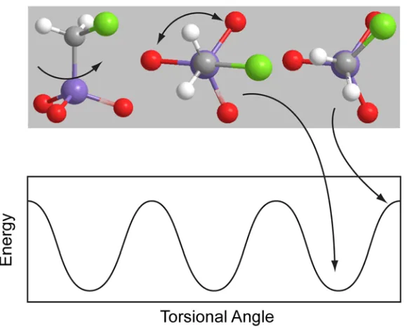
Figure 1.1: Illustration of a simple molecular rotor (top) with a
corresponding 3-fold potential diagram (bottom). ...3 Figure 1.2: Self-assembled monolayer illustrated as randomly oriented dipoles attached to a surface (top). Illustrations of the alkylsiloxane
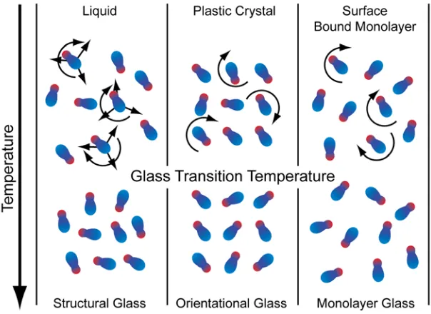
molecules attached to a surface at various densities (bottom). ...5 Figure 1.3: A liquid (top left) has translational and rotational degrees of freedom, both of which are quenched below the glass transition
(bottom left). Additionally, the density has changed. The plastic crystal (top middle) is positionally ordered and only has rotational degrees of freedom. Below the glass transition (bottom middle) this rotation is quenched. A surface bound monolayer (top right) will have rotational freedom, however this is a positionally disordered system unlike the plastic crystal. Below the glass transition (bottom right) the disorder and density remain with the rotational motion quenched. [5] ...6 Figure 1.3: Schematic of a responsive polymer surface. Upon exposure to water the hydroxyl (OH) terminated side groups migrate to the
surface. [6] ...8 Figure 2.4: Illustration of molecular orientations with corresponding potential energy graph...11 Figure 2.5: Illustration of capacitance and dissipation factor versus
temperature ...14 Figure 2.6: Equivalent circuit diagram. Here C0 represents the
capacitive components other than the molecules. The molecules are
represented by the capacitor, resistor pair, Cm and R. ...17 Figure 2.7: Illustration of the double potential well with a high
asymmetry (B=W for this illustration). ...33 Figure 2.8: Plot of Arrhenius and VFT curves. The dashed line is an
Arrhenius fitting of VFT type curve in our experimental range. The height of the grey box indicates the frequency range experimentally
vi
Figure 3.9: Illustrations of an interdigitated electrode (bottom left) and a parallel plate or “sandwich” electrode (bottom right). Additionally, side views of an interdigitated electrode (top left) and sandwich electrode (top right) with a double arrow indicated the direction
of the electric field. ...48 Figure 3.10: Illustration of the lithography process for making
interdigitated electrodes. The procedure begins at the top left and proceeds right continuing from left to right for the bottom row of
illustrations. ...50 Figure 3.11: Interdigitated electrode illustration including the width
(w), spacing (s), and coordinate system used in the electric field
calculation. ...53 Figure 3.12: Interdigitated electric field in the xy-plane above the IDE. The arrors indicate the direction and magnitude of the electric field by the color map at the top of the graph ...55 Figure 3.13: Magnitude of the electric field at the location x=0
(center of a finger pair) as a function of the distance above the
electrode. ...55 Figure 3.14: Picture of prober system and illustration of sample stage. Metal clips are used to clamp the substrate to the stage and the probes (grey trapezoids) are attached to positional manipulators
(not illustrated) and used to make non-permanent electrical contact
to the sample. ...57 Figure 3.15: Picture of chamber system and illustration of sample stage. Again metal clips are used to secure the substrate to the sample stage, however, the cold head configuration for the chamber system uses permanent contacts (as indicated by the black wires) using
silver epoxy. ...58 Figure 3.16: Simplified circuit diagram of the AH 2700A bridge.
vii
Figure 3.9: Depictions of the molecules used to form the monolayers. (a) chlorobutyldimethylchlorosilane (C4Cl (DM)),
(b) n-decyldimehtylchlorosilane (C10 (DM)),
(c) 11-bromoundecyldimethylchlorosilane (C11Br (DM)), (d) 11-bromoundecyltrichlorosilane (C11Br), and
(e) octadecyltrichlorosilane (C18). ...63 Figure 3.17: Illustration of the deposition set-up for solution phase
and vapor phase depositions. The unlabled shaded regions (blue) are the chemical solutions and the black lines represent the
deposition vessels...64 Figure 3.18: Chemical structures of the siloxane networks PVMS
and PDMS, the cross-linker TEOS, and the Merkaptoalkanol
side-chain modifiers. ...65 Figure 3.19: Simple illustration of an ellipsometer. The light source
(a He-Ne laser in our case) is polarized and reflected off the sample surface. The light then passes through an analyzer and then the
detector. ...67 Figure 3.20: Example pictures used to determine the contact angle.
The example on the bottom is more hydrophobic than that
on the top...68 Figure 4.21: Capacitance (open squares) and dissipation factor
(filled squares) at an applied field frequency of 10 kHz for PVMS.
A single relaxation is present around 155 K. ...72 Figure 4.22: Dissipation factor for PVMS at multiple frequencies:
100 Hz (triangles), 1 kHz (circles), and 10 kHz (squares). ...73 Figure 4.23: Arrhenius plot for PVMS. The natural log of the field
frequency is plotted against the inverse peak location temperature.
The red line corresponds to a VFT fit of the data. ...74 Figure 4.24: Capacitance and dissipation factor for
PVMS-S-(CH2)2-OH at 10 kHz. Two relaxations are observed
viii
Figure 4.25: Natural log of the dissipation factor vs. temperature for PVMS-S-(CH2)2-OH. The natural log was used to easily see the low temperature relaxation which has a much smaller amplitude than the high temperature relaxation. Additionally, an arbitrary y-axis offset was applied to each data set to make the individual relaxation more distinguishable. Data shown are for frequencies:
100 Hz (open diamonds), 200 Hz (filled diamonds),
1 kHz (open triangles), 2 kHz (filled triangles), 5 kHz (open circles), 10 kHz (filled circles), 16 kHz (open squares), and
20 kHz (filled squares). ...78 Figure 4.26: Arrhenius plot for low temperature relaxation.
The red line corresponds to the Arrhenius fit. ...79 Figure 4.27: Capacitance and dissipation factor plots for
PVMS-S-(CH2)6-OH at 10 kHz. At this frequency only the high
temperature relaxation is distinguishable...80 Figure 4.28: Subset of the dissipation factor data for
PVMS-S-(CH2)6-OH at 100 Hz (squares), 1 kHz (circles),
and 20 kHz (triangles). In the 100 Hz curve two relaxations are clearly seen at ~180K and ~ 240K. At 1 kHz the lower relaxation has shifted up into the higher relaxation (located at ~255 K) and is not readily seen. The 20 kHz data shows a split-peak structure with two peak
temperatures at ~240K and ~270K. ...82 Figure 4.29: Arrhenius plot for the high temperature relaxations.
The line (red) is the VFT fit of the data. ...83 Figure 4.30: Capacitance and dissipation factor for
PVMS-S-(CH2)11-OH at 10 kHz. Two relaxations are
present at ~175K and ~310K. ...85 Figure 4.31: Dissipation factor for the low temperature relaxation in
PVMS-S-(CH2)11-OH at multiple frequencies: 100 Hz (filled squares), 500 Hz (open squares), 1 kHz (filled circles), 2 kHz (open circles), 5 kHz (filled triangles), 10 kHz (open triangles),
16 kHz (filled diamonds), 20 kHz (open diamonds). ...86 Figure 4.32: Arrhenius plot for the low temperature relaxation in
ix
Figure 5.33: Comparison of vapor-deposited growth dynamics for monochlorosilane (C11Br(DM) and trichlorosilane (C11Br) molecules at 90 °C. (a) Ellipsometric measurements of film thickness versus time, where the labeled horizontal dashed line represents the maximum height of the molecule. ...97 Figure 5.34: Varying the chain length: Films grown from molecules
having 4-18 carbon atom chain lengths show a dielectric relaxation at ~235 K at 1 kHz measurement frequency: C4Cl (purple triangles), C10(DM) (black squares), C11Br(DM) (red circles), C11Br (green circles), and C18 (blue squares). The error on coverage is ± 8%. Raw data points consisting of 5 measurements at each temperature are shown; resultant point error is typically smaller than the graphed data symbols size. ...99 Figure 5.35: Arrhenius plot of ln(1/τ) versus (1/T). Data from
the ~235 K interacting relaxation is plotted for C11Br (DM) samples of 19% (upright green triangles), 42% (purple squares), and 49%
(inverted black triangles) coverage and a 99% coverage C11Br sample (blue circles). Inset: Corresponding ~150 K lower temperature relaxation from the 99% coverage C11Br sample (blue circles) and a 55%
C11Br (DM) sample (red stars). The error in the coverage is ±8%
for all samples. ...101 Figure 5.36: Varying the coverage for C11Br SAMs: Dielectric
relaxation at 1 kHz for films at sub-monolayer (58%, blue circles), monolayer (99%, green squares), and slight multilayer
(138%, red triangles) coverage. All films display a peak at ~235 K; as coverage increases, a second relaxation at ~150 K also appears. Inset: an expanded view of the 58% C11Br SAM showing only the
~ 235 K relaxation. Raw data points consisting of 5 measurements at each temperature are shown;resultant point error is typically smaller than the graphed data symbols size. The error in the coverage is ±8%
x
Figure 5.37: Dielectric spectroscopy of a full coverage (99%)
C11Br SAM. Loss (left axis, tan(δ)) measured with applied frequencies of 0.1, 0.5, 1, 2, 10, 16, and 20 kHz as a function of sample temperature. Representative vertical lines at 0.1 and 20 kHz are drawn at each lower temperature maximum, respectively, to aid the eye in demonstrating the dispersive nature of the relaxation. Raw data points consisting of 5 measurements at each temperature are shown; resultant point error is typically smaller than the graphed data symbols size. The corresponding step-wise change is shown in the capacitance for 1 kHz (right axis
(open circles)). ...109 Figure 6.38: Dielectric spectra at 1 kHz for C11Br at 65% coverage
(open squares), C11Br at 18% coverage (open triangles), C11Br (DM) at 35% coverage (open circles), and C11Br (DM) at 6.9% coverage (open diamonds). In the legend, TC designates trichloro (three feet)
and DM designates dimethyl (single foot). ...114 Figure 6.39: Arrhenius plot for C11Br samples of varying coverage:
5.5 % (filled squares), 41% (open circles), 75 % (filled triangles), 23 % (open diamonds), 63 % (filled circles), 99 % (open squares),
and 78% (filled diamonds). ...116 Figure 6.40: Glass transition temperature as determined by VFT fits
for C11Br. As a reference point the glass transition temperature for polyethylene and liquid undecane are indicated by their respectively labeled horizontal lines. ...117 Figure 6.41: Plot of the fragility (m) for various densities of C11B
1
Chapter 1-Introduction
2
and time scales of a certain motion are not necessarily exclusive to that motion. This flexibility is fundamental to the properties that make polymeric materials so highly useful for the myriad applications in which they are used (and their ubiquitous place in modern life), but it also contributes to the difficulties in the scientific study of these materials.
3
Figure 1.1: Illustration of a simple molecular rotor (top) with a corresponding 3-fold potential diagram (bottom).
4
A primary motivation for investigating systems of surface-bound molecules, described above, is that polymer dynamics tend to be very complex for even a single molecule. Also, experimentally, it is often a large collection of interacting molecules under study, which modifies their dynamics (giving it, for instance, a more complicated temperature dependence) and further increases the difficulty in understanding polymer dynamics. In fact, it is this interaction that leads to the presence of the glass transition temperature, below which dynamics are dramatically quenched. Because of the great complexity of the system, the glass transition, as described above, remains one of the fundamental unsolved problems in condensed matter physics. The molecular interaction for our surface-bound molecules however, can be controlled in an explicit way by changing the density of the system. We utilize self-assembled monolayer chemistry to fabricate these samples, which results in molecules randomly positioned on a substrate. Each molecule is tethered to the surface to minimize its translational motion, and the number of surface-bound molecules (i.e. sample density) can be explicitly controlled.
5
Figure 1.2: Self-assembled monolayer illustrated as randomly oriented dipoles attached to a surface (top). Illustrations of the alkylsiloxane molecules attached to a surface at various densities (bottom).
6
samples system represents a complementary model to this work. The specifics of the self-assembled monolayers used are found in Section 3.3.
Figure 1.3: A liquid (top left) has translational and rotational degrees of freedom, both of which are quenched below the glass transition (bottom left). Additionally, the density has changed. The plastic crystal (top middle) is positionally ordered and only has rotational degrees of freedom. Below the glass transition (bottom middle) this rotation is quenched. A surface bound monolayer (top right) will have rotational freedom, however this is a positionally disordered system unlike the plastic crystal. Below the glass transition (bottom right) the disorder and density remain with the rotational motion quenched. [5]
7
8
9
Chapter 2-Dielectric Relaxation Theory
Dielectric spectroscopy is a technique which allows observation of the dynamics of molecules in the hertz to megahertz range. This technique has been used since the 1950’s to characterize molecular motion in a variety of systems, in particular it has been extensively used by the polymer community [7--9]. Besides being a well established experimental technique, advances in capacitance bridge design and sensitivity allow for the application of dielectric spectroscopy to systems containing relatively small numbers of molecules. This is particularly useful for the research presented on self-assembled monolayer systems, where techniques such as dynamical mechanical analysis (DMA) could not be used.
10
Before delving into the mathematical derivations, it is beneficial to provide a cursory examination of how the molecular motion may present itself in both the capacitance and dissipation factor. Capacitance is proportional to the polarization of the system; that is, how many dipoles are aligned in the direction of some applied electric field. The concept of loss is less familiar. Technically, the dissipation factor, tan(δ), measures the phase angle between the applied voltage and the measured current. For an ideal capacitor there is no loss; that is, the current will be exactly 90° out of phase to the voltage. A real capacitor, however, contains resistive or lossy components that will change this phase difference.
11
Figure 2.1: Illustration of molecular orientations with corresponding potential energy graph.
12
and the energy of the potential well (W). The relation of the energies typically follow pE (4-8 x10⁻⁴ kcal/mol) <kT (0.2-0.8 kcal/mol) <<W (3-10 kcal/mol).
Based on these energy scales, the effect of the applied electric field is to slightly perturb the system so that the positions where the molecular dipole is aligned (counter-aligned) with the electric field are slightly lower (higher) in energy. This is in contrast to the driven regime, in which field-dipole interaction energy is on the order of the barrier to motion and thus the electric field causes the motion. In the work presented here, the dipole-electric field coupling serves only the highlight the innate thermal motion, which is present with or without the electric field.
In addition to the energies of the system there are two frequencies of importance: the frequency of the applied electric field (ωE), and the frequency of the thermally activated hopping (ωm). In our measurements, we set ωE and tune ωm by adjusting the temperature of the system. As the thermal energy of the system is increased the relation between these two frequencies will be in one of three regimes: ωm < ωE, ωm ≈ ωE, and ωm > ωE. These three regimes will manifest themselves in both the capacitance and the dissipation factor of the sample. Figure 2.2 illustrates the general shape for both of these measurements.
13
14
Figure 2.2: Illustration of capacitance and dissipation factor versus temperature
2.1- Equivalent circuit model
15
and a resistor R arranged in series together. This reflects both the charge storage (polarization) ability of the molecules (in Cm) and their dissipative nature (in R). In addition, RC is the characteristic response time for the molecular system. This molecular element pair is arranged in parallel with C0, as both the molecules and the other elements of the capacitor (air, substrate) experience the same voltage drop. The circuit diagram is shown in Figure 2.3. Using Kirchhoff’s laws two differential equations may be determined:
𝑄𝑄0 =𝐶𝐶0𝑉𝑉 ( 2.1)
𝑅𝑅𝐶𝐶𝑚𝑚 𝑑𝑑𝑄𝑄𝑑𝑑𝑑𝑑𝑚𝑚 +𝑄𝑄𝑚𝑚 =𝐶𝐶𝑚𝑚𝑉𝑉. ( 2.2)
Combining the two equations results in
𝑅𝑅𝐶𝐶𝑚𝑚 𝑑𝑑𝑄𝑄𝑑𝑑𝑑𝑑𝑚𝑚 +𝑄𝑄𝑚𝑚 +𝑄𝑄0 =𝐶𝐶𝑚𝑚𝑉𝑉+𝐶𝐶0𝑉𝑉. ( 2.3)
Rearranging of the equation and using Q=Qm+Q0 allows Eq. 2.3 to be written as
𝜏𝜏𝑑𝑑𝑄𝑄
𝑑𝑑𝑑𝑑 =−𝑄𝑄+ (𝐶𝐶𝑚𝑚 +𝐶𝐶0)𝑉𝑉+𝜏𝜏𝐶𝐶0 𝑑𝑑𝑉𝑉
𝑑𝑑𝑑𝑑 ( 2.4)
where 𝜏𝜏 =𝑅𝑅𝐶𝐶𝑚𝑚. The solution to Eq. 2.4 may be found by substituting the complex voltage 𝑉𝑉 =𝑉𝑉𝑖𝑖e−𝑖𝑖𝑖𝑖𝑑𝑑and complex charge 𝑄𝑄 =𝑄𝑄𝑖𝑖e−𝑖𝑖𝑖𝑖𝑑𝑑 and solving for the capacitance C=Q/V. The
16 𝐶𝐶∗ =𝐶𝐶0 +𝐶𝐶𝑚𝑚 − 𝑖𝑖𝑖𝑖𝜏𝜏𝐶𝐶0
1− 𝑖𝑖𝑖𝑖𝜏𝜏 =𝐶𝐶0 + 𝐶𝐶𝑚𝑚
1− 𝑖𝑖𝑖𝑖𝜏𝜏 ( 2.5)
The real and imaginary parts of the capacitance are,
𝐶𝐶′ =𝐶𝐶
0 +1 +𝐶𝐶𝑖𝑖𝑚𝑚2𝜏𝜏2 𝐶𝐶′′ = 𝐶𝐶𝑚𝑚𝑖𝑖𝜏𝜏
1 +𝑖𝑖2𝜏𝜏2
( 2.6)
with the dissipation factor
tan𝛿𝛿 =𝐶𝐶𝐶𝐶′′′ =𝐶𝐶𝐶𝐶𝑚𝑚
0
𝑖𝑖𝜏𝜏
1 +𝑖𝑖2𝜏𝜏2 ( 2.7)
17
Figure 2.3: Equivalent circuit diagram. Here C0 represents the capacitive components other than the molecules. The molecules are represented by the capacitor, resistor pair, Cm and R.
In our experimental set up, the observable quantities come from equations 2.6 (C’) and 2.7, and the limits of these equations can be examined in comparison to the general line shapes found in Figure 2.2. Beginning with the real part of the capacitance (top equation in 2.6), at low temperatures τ (which represents the average relaxation time of the molecules) will be large in comparison to 1/ω. This results in the Cm term being small and 𝐶𝐶′ ≅ 𝐶𝐶0. Thus, the molecules are not contributing to the capacitance. As the temperature increases, τ will decrease and at some temperature 𝑖𝑖𝜏𝜏= 1 and 𝐶𝐶′ ≅ 𝐶𝐶0+𝐶𝐶𝑚𝑚
2 . Further increases in the temperature result in τ continuing to decrease and 𝐶𝐶′ ≅ 𝐶𝐶0+𝐶𝐶𝑚𝑚, resulting in the capacitance step seen in Figure 2.2. Using the same relations between ω and τ and examining equation 2.7 for tan(δ), at low temperatures tan𝛿𝛿 ≅𝐶𝐶𝑚𝑚
𝐶𝐶0
1
𝑖𝑖𝜏𝜏 where
1
𝑖𝑖𝜏𝜏 will be a small number. Thus
18
tan(𝛿𝛿)≅ 𝐶𝐶𝑚𝑚 𝐶𝐶0
1
2, and at high temperatures tan𝛿𝛿 ≅
𝐶𝐶𝑚𝑚
𝐶𝐶0𝑖𝑖𝜏𝜏, with 𝑖𝑖𝜏𝜏 being small in comparison
to ½. Thus one advantage of the tan(δ) measurement is that it manifests a peak at 𝑖𝑖𝜏𝜏 = 1 surrounded by regions where tan(δ) is almost zero at high and low temperatures. As we shall see later, the presence of other relaxations and of ionic conductivity (which, if present, increases exponentially with temperature) complicate this simple picture. These limits are presented in Table 2.1. and correspond to the regions depicted in Figure 2.2.
Table 2.1: Approximations of the capacitance and dissipation factor for low, moderate, and high temperature regimes.
Low Temperature 𝜏𝜏 ≫ 𝑖𝑖
Moderate Temperature
𝑖𝑖𝜏𝜏 = 1
High Temperature 𝜏𝜏 ≪ 𝑖𝑖 Real part of
Capacitance 𝐶𝐶′ =𝐶𝐶
0+1 +𝐶𝐶𝑖𝑖𝑚𝑚2𝜏𝜏2 𝐶𝐶′ ≅ 𝐶𝐶0 𝐶𝐶
′ ≅ 𝐶𝐶
0+𝐶𝐶2𝑚𝑚 𝐶𝐶′ ≅ 𝐶𝐶0+𝐶𝐶𝑚𝑚
Dissipation Factor
tan𝛿𝛿=𝐶𝐶𝐶𝐶𝑚𝑚
0
𝑖𝑖𝜏𝜏
1 +𝑖𝑖2𝜏𝜏2 tan𝛿𝛿 ≅
𝐶𝐶𝑚𝑚
𝐶𝐶0
1
𝑖𝑖𝜏𝜏 tan𝛿𝛿 ≅ 𝐶𝐶𝑚𝑚
𝐶𝐶0
1
2 tan𝛿𝛿 ≅
𝐶𝐶𝑚𝑚
𝐶𝐶0 𝑖𝑖𝜏𝜏
2.2-Molecular Formulation of Debye Model
19
advantageous, then, to derive the Debye equation from a molecular standpoint. Additional sources for the following derivation include Daniel’s Dielectric Relaxation [10] and Frölich’s Theory of Dielectrics [11]. The derivation begins with the static electric field of a capacitor in vacuum,
𝐸𝐸 = 4𝜋𝜋𝜎𝜎0, ( 2.8)
where 𝜎𝜎0 is the charge density per area on the capacitor plates. If a dielectric is inserted into the capacitor, the charge is altered and now equal to
𝜎𝜎 =𝜖𝜖𝑚𝑚𝜎𝜎0, ( 2.9)
where 𝜖𝜖𝑚𝑚 is the dielectric constant (the subscript m is maintained from the previous derivation as experimentally the dielectric inserted is the molecules being measured). This leads to the displacement field
𝐷𝐷 = 4𝜋𝜋𝜎𝜎 =𝜖𝜖𝑚𝑚𝐸𝐸 =𝐸𝐸+ 4𝜋𝜋𝜋𝜋 where 𝜋𝜋 =𝜎𝜎 − 𝜎𝜎0. ( 2.10)
In the above equation E is the electric field and P is the polarization density (referred to as polarization for the remainder of this discussion). Using Eq. 2.10 the dielectric constant can be defined in terms of the polarization P resulting in
20
Before examining the time dependence it is prudent to further examine Eq. 2.11 and distinguish between types of polarizations. Possible polarizations to consider may be classified into the following groups: electronic, ionic, and motion of permanent dipoles. Electronic polarization is the displacement of the electrons in an atom and typically occurs at frequencies (> 1012 Hz) far above those typically utilized in electrical measurements. Our measurements are in the 100 Hz to 20 kHz range. Ionic polarization is found in ion containing materials which under the influence of an electric field will displace the ion position resulting in a net polarization for the material. This process is much slower than electronic polarization. The motion of permanent dipoles is the type of polarization studied in this thesis and is a result of the reorientation of permanent dipoles in a material. As electronic polarization can always be present and assuming that all materials of interest will also contain permanent dipoles (though excluding ionic polarization) Eq. 2.11 may be rewritten as
𝜖𝜖𝑚𝑚 −1 =4𝐸𝐸𝜋𝜋(𝜋𝜋𝐷𝐷 +𝜋𝜋∞) with 𝜖𝜖∞ −1 =4𝜋𝜋𝜋𝜋𝐸𝐸∞. ( 2.12)
21
The response of a material system to a time dependent electric field can be determined by assuming that the rate by which the time dependent polarization approaches equilibrium is proportional to the distance from equilibrium, resulting in
𝜏𝜏𝑑𝑑𝜋𝜋𝑑𝑑𝑑𝑑(𝑑𝑑)=𝜋𝜋𝑠𝑠𝑑𝑑𝑠𝑠𝑑𝑑𝑖𝑖𝑠𝑠 − 𝜋𝜋(𝑑𝑑) ( 2.13)
This is a standard assumption for any process relaxing towards equilibrium, and is derived from the physical argument in the next paragraph. Applying Eq. 2.13 to the dipolar polarization gives
𝜏𝜏𝑑𝑑𝜋𝜋𝑑𝑑𝑑𝑑𝐷𝐷 +𝜋𝜋𝐷𝐷(𝑑𝑑) = (𝜖𝜖𝑚𝑚 − 𝜖𝜖∞)𝐸𝐸4(𝜋𝜋𝑑𝑑) ( 2.14)
For a periodic electric field (using Eq. 2.12) the solution to Eq. 2.14 is
𝜋𝜋𝐷𝐷 =𝐾𝐾𝑒𝑒−
1
𝜏𝜏 + 1
4𝜋𝜋
𝜖𝜖𝑚𝑚 − 𝜖𝜖∞
1 +𝑖𝑖𝑖𝑖𝜏𝜏 𝐸𝐸0𝑒𝑒𝑖𝑖𝑖𝑖𝑑𝑑, ( 2.15)
22 𝜖𝜖∗− 𝜖𝜖
∞ = 4𝜋𝜋𝜋𝜋𝐷𝐷 ∗
𝐸𝐸∗ =
𝜖𝜖𝑚𝑚 − 𝜖𝜖∞
1 +𝑖𝑖𝑖𝑖𝜏𝜏 ( 2.16)
Separating Eq. 2.16 into the real and imaginary components result in
𝜖𝜖′ =𝜖𝜖
∞ +1 +𝜖𝜖𝑚𝑚 − 𝜖𝜖𝑖𝑖2𝜏𝜏∞2
𝜖𝜖′′ = (𝜖𝜖
𝑚𝑚 − 𝜖𝜖∞)1 +𝑖𝑖𝜏𝜏𝑖𝑖2𝜏𝜏2
. ( 2.17)
The dissipation factor may be defined in terms of the dielectric constant as
tan𝛿𝛿 =𝐶𝐶𝐶𝐶′′′ =𝜒𝜒𝜒𝜒′′′ =𝜖𝜖𝜖𝜖′′′ =𝜖𝜖(𝜖𝜖𝑚𝑚 − 𝜖𝜖∞)𝑖𝑖𝜏𝜏
𝑚𝑚 +𝜖𝜖∞𝑖𝑖2𝜏𝜏2,
( 2.18)
obtaining the same form as Eq. 2.7.
23
transition rate can be quantified via transition-state theory (TST), which examines rates for any physical system where two stable equilibriums are separated by a potential barrier, which can be overcome via thermal fluctuations. For instance, one well could represent the energy of the reactants and the other the energy of the products for a chemical reaction. Though TST was developed, using statistical mechanics, to, in part, examine the rates of chemical reactions, these rates can be successfully applied to other transitional processes where a free energy barrier exists, such as molecular hopping between wells.
The rate equation developed by Eyring [12],
𝑘𝑘 =𝑘𝑘𝑏𝑏𝑇𝑇
ℎ exp�−
Δ𝐺𝐺‡
𝑅𝑅𝑇𝑇�, ( 2.19)
will serve as the basis for the rate equation used in this work. In the Eyring equation k is the rate of the process, kb is the Boltzmann constant, h is Plank’s constant, T the temperature, R the gas constant, and ΔG‡ is the Gibbs free energy of activation; where Δ𝐺𝐺‡=Δ𝐻𝐻 − 𝑇𝑇Δ𝑆𝑆 = Δ𝐸𝐸+𝑝𝑝Δ𝑉𝑉 − 𝑇𝑇Δ𝑆𝑆 with ΔE the change in internal energy, ΔV the change in volume, and ΔS the change in entropy. In applying Eq. 2.19 to molecular reorientation some simplifications can be made. First the linear temperature dependence in the pre-factor, 𝑘𝑘𝑏𝑏𝑇𝑇
ℎ , will not be as
24
temperature independent constant, ω0. This is a common approximation. Secondly, the exponential term can be simplified by examining the Gibbs free energy. For our physical system the two wells represent a molecule which has reoriented by 180°. Whereas in a chemical reaction, the volume could change dramatically, due to a phase change, volume changes will be minimal for a simple molecular reorientation. Similarly, for a chemical reaction, the total entropy of the system can also be significantly altered (again by phase transitions) or due to the change in the number of species (two small molecules becoming a larger molecule). There should be no change in entropy, however, for a randomly reorienting system of molecules. (Providing that the molecules are non-interacting as we have assumed here. We discuss this issue later in Section 2.3.) For these reasonsΔ𝐺𝐺‡≅ Δ𝐸𝐸, and in subsequent equations ΔE will be referred to as W relating to the previous notation for the barrier to motion. Making the approximations to Eq. 2.19 results in the Arrhenius equation
1
𝜏𝜏 =𝑖𝑖0exp�− 𝑊𝑊 𝑘𝑘𝑏𝑏𝑇𝑇�,
( 2.20)
25
Eq. 2.20 must be modified to account for the applied electric field, which is not necessarily in the direction of the dipole, and also to account for any innate asymmetry of the two potential that may exist. For the moment, we assume a single dipole with a well-defined angle to the field. The hopping rates are now
1/𝜏𝜏12 =𝑖𝑖0exp�
−𝑊𝑊+𝐵𝐵2− 𝑝𝑝𝐸𝐸cos𝜃𝜃
𝑘𝑘𝑇𝑇 �
1/𝜏𝜏21 =𝑖𝑖0exp�
−𝑊𝑊 − 𝐵𝐵2 +𝑝𝑝𝐸𝐸cos𝜃𝜃
𝑘𝑘𝑇𝑇 �
( 2.21)
where θ is the angle between the electric field E and the dipole moment p and B is an intrinsic asymmetry (if present) between the two potential wells. 1/τij is the rate of hopping from well i to well j. From a master equation approach, the change in the number of dipoles in well 1 will consist of the dipoles transitioning from well 2 to 1 minus those transitioning from well 1 to 2:
𝑑𝑑𝑁𝑁1
𝑑𝑑𝑑𝑑 =−𝑁𝑁1/𝜏𝜏12 +𝑁𝑁2/𝜏𝜏21. ( 2.22)
In addition,
𝑑𝑑𝑁𝑁1 𝑑𝑑𝑑𝑑 =−
𝑑𝑑𝑁𝑁2
26 because 𝑑𝑑𝑁𝑁
𝑑𝑑𝑑𝑑 = 0 where 𝑁𝑁 =𝑁𝑁1+𝑁𝑁2. Equivalently,
𝑁𝑁1/𝜏𝜏12 =𝑁𝑁2/𝜏𝜏21 with 𝑁𝑁1 +𝑁𝑁2 =𝑁𝑁. ( 2.24)
Eq. 2.23 and Eq. 2.24 give the result 𝑑𝑑(𝑁𝑁1− 𝑁𝑁2)
𝑑𝑑𝑑𝑑 = 2
𝑑𝑑𝑁𝑁1
𝑑𝑑𝑑𝑑 . ( 2.25)
The quantity N1-N2 is important because it is related to the polarization. The definition of the polarization is 𝜋𝜋 = (𝜂𝜂1− 𝜂𝜂2)𝑝𝑝cos(𝜃𝜃), where 𝑝𝑝cos(𝜃𝜃) is the projection of the dipole along (or against) the electric field and η1-η2 counts the net number of dipoles per volume along the field (as the polarization is a per volume quantity, η is used in place of N which was defined as the number of dipoles, not the number per volume). Using Eq. 2.22, and this definition, Eq. 2.25 can be rewritten as
1 2𝑝𝑝cos(𝜃𝜃)
𝑑𝑑𝜋𝜋 𝑑𝑑𝑑𝑑 =−
𝜂𝜂1 𝜏𝜏12 +
𝜂𝜂2 𝜏𝜏21 .
( 2.26)
27
the hopping rates will not be introduced so as to make the derivation easier to read and follow. Proceeding from Eq. 2.26, and using the relationship η=η1+η2 results in
1
2𝑝𝑝cos(𝜃𝜃)𝑑𝑑𝜋𝜋𝑑𝑑𝑑𝑑 =−(𝜂𝜂 − 𝜂𝜂2)�
1
𝜏𝜏12�+𝜂𝜂2�
1
𝜏𝜏21�.
1 2𝑝𝑝cos(𝜃𝜃)
𝑑𝑑𝜋𝜋
𝑑𝑑𝑑𝑑 =−𝜂𝜂1�
1
𝜏𝜏12�+ (𝜂𝜂 − 𝜂𝜂1)�
1
𝜏𝜏21�.
( 2.27)
Again for clarity, the 1/τij terms will be replaced by ωij and care should be taken to not confuse these terms with the electric field frequency ω which will be later introduced into these equations. Continuing by adding the two above equations
1
𝑝𝑝cos(𝜃𝜃)
𝑑𝑑𝜋𝜋
𝑑𝑑𝑑𝑑 =𝜂𝜂(𝑖𝑖21 − 𝑖𝑖12) + (𝑖𝑖21 +𝑖𝑖12)(𝜂𝜂2− 𝜂𝜂1), ( 2.28)
and dividing by the sum of the hopping rates so the polarization term may be recovered on the right hand side of the equation results in
1
𝑝𝑝cos(𝜃𝜃)
1
𝑖𝑖21 +𝑖𝑖12 𝑑𝑑𝜋𝜋
𝑑𝑑𝑑𝑑 =
𝜂𝜂(𝑖𝑖21 − 𝑖𝑖12) 𝑖𝑖21 +𝑖𝑖12 −
(𝜂𝜂1− 𝜂𝜂2)(𝑖𝑖21+𝑖𝑖12) 𝑖𝑖21 +𝑖𝑖12 .
( 2.29)
Multiplying by the dipole component we arrive at
1
𝑖𝑖21 +𝑖𝑖12 𝑑𝑑𝜋𝜋
𝑑𝑑𝑑𝑑 =𝑝𝑝cos(𝜃𝜃)
𝜂𝜂(𝑖𝑖21 − 𝑖𝑖12) 𝑖𝑖21 +𝑖𝑖12 − 𝜋𝜋.
28
Comparison with Eq. 2.13 shows the relaxation time for the system to be 𝜏𝜏 = 1
𝑖𝑖21+𝑖𝑖12, and
the static polarization to be 𝑝𝑝cos(𝜃𝜃)𝜂𝜂(𝑖𝑖21−𝑖𝑖12)
𝑖𝑖21+𝑖𝑖12 .
The static polarization will be addressed shortly, but we first examine the relaxation time by substituting the full forms of the hopping frequencies,
𝜏𝜏 = 1
𝑖𝑖0exp�
−𝑊𝑊+𝐵𝐵2 − 𝑝𝑝𝐸𝐸cos𝜃𝜃
𝑘𝑘𝑇𝑇 �+𝑖𝑖0exp�
−𝑊𝑊 − 𝐵𝐵2 +𝑝𝑝𝐸𝐸cos𝜃𝜃
𝑘𝑘𝑇𝑇 �
.
( 2.31)
With factoring common terms,
𝜏𝜏 = 1
𝑖𝑖0exp�− 𝑊𝑊𝑘𝑘𝑇𝑇�
1 exp�
𝐵𝐵
2− 𝑝𝑝𝐸𝐸cos𝜃𝜃
𝑘𝑘𝑇𝑇 �+ exp�
− 𝐵𝐵2 +𝑝𝑝𝐸𝐸cos𝜃𝜃
𝑘𝑘𝑇𝑇 �
.
( 2.32)
29
We first examine the case where the hopping rates between the two wells are equal (τ12=τ21=τ0) by setting B=0 and E=0 resulting in
𝜏𝜏= 1
2𝑖𝑖0exp�− 𝑊𝑊𝑘𝑘𝑇𝑇�
=𝜏𝜏2ℎ. ( 2.33)
Again, τ is the relaxation time of the system and τh is the hopping time. In this case, the relaxation time is one half of the hopping time, which is now equal to the Arrhenius equation (Eq. 2.20). This would be the experimentally observed relaxation time for the system’s polarization upon application of an electric field.
30
If we now release the constraint that the electric field is zero (still leaving the innate asymmetry aside)
𝜏𝜏 = 1
𝑖𝑖0exp�− 𝑊𝑊𝑘𝑘𝑇𝑇�
1
exp�−𝑝𝑝𝐸𝐸𝑘𝑘𝑇𝑇cos𝜃𝜃�+ exp�+𝑝𝑝𝐸𝐸𝑘𝑘𝑇𝑇cos𝜃𝜃� . ( 2.34)
As is the case for our experiments, we can consider that 𝑝𝑝𝐸𝐸cos(𝜃𝜃)≪ 𝑘𝑘𝑇𝑇 and the relaxation time can be approximated as
𝜏𝜏 ≅ 1
𝑖𝑖0exp�− 𝑊𝑊𝑘𝑘𝑇𝑇�
1
2 . ( 2.35)
The ½ is a result of a Taylor series expansion of the E dependent term about zero. In this approximation we have recovered the same relaxation time as when the electric field is equal to zero. This indicates that to the first order, our electric field does not influence the hopping rate of the molecules. In this sense it is a non-perturbative probe of the innate dynamics of the system enabling (through the generation of an experimentally measureable, but very small polarization) detection of the dynamics of the system without altering them. Note that this would not be true if pE was a larger quantity; in particular if pE were large enough (similar to W), the electric field would first perturb and then dominate the dynamics of the system.
31
𝜏𝜏 = 1
𝑖𝑖0exp�− 𝑊𝑊𝑘𝑘𝑇𝑇�
1
exp� −𝐵𝐵2𝑘𝑘𝑇𝑇�+ exp�2+𝑘𝑘𝑇𝑇�𝐵𝐵 . ( 2.36)
This equation can also be written as 1/(𝑖𝑖12 +𝑖𝑖21). For any significant B (larger than a few kT) it is obvious that ω12 will not be close to ω21. Thus hopping out of the higher energy well, which now has a reduced barrier, will be much faster than hopping out of the lower energy well, which now has an enhanced barrier. The B containing terms in Eq. 2.36 can be expressed as sech� 𝐵𝐵
2𝑘𝑘𝑇𝑇� which affects the total observable polarization as discussed below.
The illustration in Figure 2.4 shows a potential with a large asymmetry and in this case the hopping from 1 to 2 will be much slower than from 2 to 1. In the situation where B=2W (a very extreme case) the relaxation time of the system is now
𝜏𝜏 = 1
𝑖𝑖0�exp�−2𝑘𝑘𝑇𝑇 �𝑊𝑊 + 1�
. ( 2.37)
Comparison with Eq. 2.34, where B=0 and E=0, results in τB=2W < τB=0. This means that the dynamics are significantly faster (lower τ values) when asymmetry is present, reflecting the lower effective barrier (hopping from the higher energy well). In the regime where the two wells differ significantly in energy, 𝜏𝜏= 1
𝑖𝑖21+𝑖𝑖12 becomes 𝜏𝜏 = 1/𝑖𝑖𝑓𝑓𝑠𝑠𝑠𝑠𝑑𝑑 where 1/ωfast is the
32
33
Figure 2.4: Illustration of the double potential well with a high asymmetry (B=W for this illustration).
To quantify the effects discussed above we will further examine the polarization and beginning from Eq. 2.30
𝜋𝜋 =𝑝𝑝cos(𝜃𝜃)𝜂𝜂(𝑖𝑖21 − 𝑖𝑖12)
𝑖𝑖21 +𝑖𝑖12 =𝜂𝜂𝑝𝑝cos(𝜃𝜃)tanh� 𝐵𝐵
2− 𝑝𝑝cos(𝜃𝜃)𝐸𝐸
34
The hyperbolic tangent in the above equation serves to represent an important physical result. For simplicity, if B=0 then 𝜋𝜋 =𝜂𝜂𝑝𝑝cos(𝜃𝜃)tanh�−𝑝𝑝cos(𝜃𝜃)𝐸𝐸
𝑘𝑘𝑇𝑇 �. As the strength of the electric
field increases so will the polarization. At small values of E/kT (approximation shown below) the response in the polarization will be linear to an increase in the electric field. However, if E becomes very large the polarization saturates and 𝜋𝜋 =𝜂𝜂cos(𝜃𝜃). At this point, all dipoles are generally aligned with the field and thus further field increases result in little increase in polarization. In our work, we are far from this limit; in this case, pE would be large. That is, the electric field would no longer be probing the dynamics of the system, but instead driving them. The pE/kT term in hyperbolic tangent term is worth discussion. Random thermal motion (as quantified by kT) will generally fight against the alignment of the dipole with the electric field. Thus as kT increases the maximum possible polarization decreases. In the saturation regime, as pE increases, the polarization increases slightly as the quantity pE/kT further increases. In the linear regime, discussed below, this term pE/nkT, where n is a numerical factor, depending on the dimensionality of the system, is referred to as the Curie factor, from its first use in paramagnetic system (rather than the paraelectric system under study here).
Applying the approximation that 𝑝𝑝𝐸𝐸cos(𝜃𝜃)≪ 𝑘𝑘𝑇𝑇 results in
𝜋𝜋 =𝜂𝜂𝑝𝑝cos(𝜃𝜃)�tanh� 𝐵𝐵
2𝑘𝑘𝑇𝑇� −
𝑝𝑝cos(𝜃𝜃)𝐸𝐸
𝑘𝑘𝑇𝑇 sech2� 𝐵𝐵
35
The cos(θ) term was first introduced with the assumption of all dipoles in the system having the same angle to (or 180° from) the electric field. This is not consistent with our experimental system where the molecules are randomly oriented with respect to the field. These terms would be important for an ordered dipolar system, such as a ferroelectric. If this constraint is released and dipoles can be in any orientation (uniformly distributed), an average polarization in the direction of the electric field can be calculated by averaging over the solid angle (sin(θ)dθdφ). Before altering Eq. 2.39 the two terms should be examined. The hyperbolic tangent represents a non-responsive (to the electric field) term due to the innate asymmetry in the potential. This will go away after averaging, since each of these preferred dipolar positions is in a random direction and thus it leads to no net polarization. The second term will remain present and is the dipolar response to the applied field. In this second term there is a hyperbolic secant factor of the potential asymmetry. As the asymmetry increases it serves to reduce this second term and thus the polarization, as discussed in the previous paragraph. While this second term is being reduced the first non-responsive term gets larger, however as stated this goes away upon angular averaging. After averaging over orientation, the polarization is
𝜋𝜋 =𝜂𝜂𝑝𝑝3𝑘𝑘𝑇𝑇2𝐸𝐸sech2� 𝐵𝐵
36
The factor pE/3kT introduced in this approximation is known as the Curie factor, as discussed above.
One more correction needs to be made before solving Eq. 2.30. As a final detail, we can also consider that the electric field experienced by the dipoles will be screened by the surrounding material. This is a classical correction. Consider the electric field in the space between dipoles as
𝐸𝐸𝑖𝑖 =𝐸𝐸+43𝜋𝜋𝜋𝜋, ( 2.41)
where E is the applied electric field and 4𝜋𝜋
3 𝜋𝜋 is contribution from the local field for a spherical volume around a dipole.
Now defining 𝜋𝜋𝑠𝑠 = 𝜋𝜋𝐷𝐷+𝜋𝜋∞ = (𝛼𝛼𝐷𝐷 +𝛼𝛼∞)𝐸𝐸𝑖𝑖 where αD and α∞ are the dipolar and optical polarizabilities respectfully, and using Eq. 2.12,
𝜖𝜖𝑚𝑚 −1
𝜖𝜖𝑚𝑚 + 2=
4𝜋𝜋
3 (𝛼𝛼𝐷𝐷 +𝛼𝛼∞). ( 2.42)
Rearranging the above equation results in
𝜖𝜖𝑚𝑚 −1 =𝜖𝜖𝑚𝑚3+ 2 4𝜋𝜋𝐸𝐸𝜋𝜋𝑠𝑠 𝑖𝑖,
37
which is equivalent to Eq. 2.11 for the modified electric field by a factor of 𝜖𝜖𝑚𝑚+2
3 . This factor can then be brought into equation 2.30 as
𝜏𝜏𝑑𝑑𝜋𝜋 𝑑𝑑𝑑𝑑 =
𝜖𝜖𝑚𝑚 + 2
3
𝜂𝜂𝑝𝑝2𝐸𝐸
3𝑘𝑘𝑇𝑇 sech2� 𝐵𝐵
2𝑘𝑘𝑇𝑇� − 𝜋𝜋, ( 2.44)
Where the derived static polarization 2.40 has been included with the factor from 2.43 and again τ is the system relaxation rate and P is the polarization.
Following the same derivation from Eq. 2.11 with an alternating electric field the complex dielectric constant is
𝜖𝜖∗=𝜖𝜖𝑚𝑚+ 2
3 𝜂𝜂𝑝𝑝
2𝐸𝐸
3𝑘𝑘𝑇𝑇 sech2�2𝐵𝐵𝑘𝑘𝑇𝑇�1 +1𝑖𝑖𝑖𝑖𝜏𝜏+𝜖𝜖∞, ( 2.45)
recalling that εm is the dielectric constant with the optical component represented by
ε∞. As well, ω is the frequency of the applied field and τ is the relaxation time of the system. To relate back to the equivalent circuit derivation the real and imaginary parts are put in terms of the capacitance as,
𝐶𝐶′ =𝐶𝐶
0+𝜖𝜖𝑚𝑚3+ 2𝜂𝜂𝑝𝑝 2𝐸𝐸
3𝑘𝑘𝑇𝑇 sech2�2𝐵𝐵𝑘𝑘𝑇𝑇�1 +1𝑖𝑖2𝜏𝜏2
𝐶𝐶′′ =𝜖𝜖𝑚𝑚+ 2
3 𝜂𝜂𝑝𝑝
2𝐸𝐸
3𝑘𝑘𝑇𝑇 sech2�2𝐵𝐵𝑘𝑘𝑇𝑇�1 +𝑖𝑖𝜏𝜏𝑖𝑖2𝜏𝜏2
38 which is equivalent to 2.6 with
𝐶𝐶𝑚𝑚 =𝜖𝜖𝑟𝑟3+ 2𝜂𝜂𝑝𝑝
2𝐸𝐸
3𝑘𝑘𝑇𝑇 sech2� 𝐵𝐵
2𝑘𝑘𝑇𝑇�. ( 2.47)
When analyzing data Eq. 2.47 is a primary tool. To review, the first fraction reflects the screening of the electric field by the surrounding dipoles, which is derived for a three-dimensional system, where each dipole is surrounded by other dipoles. This term is generally less important in two-dimensional systems. The second term includes the number density of molecules (η) and the size of the dipole moment (p), each of which should increase Cm. In addition, the second fraction includes the term pE/3kT, which resulted from approximating the hyperbolic tangent to the limit 𝑝𝑝𝐸𝐸 ≪ 𝑘𝑘𝑇𝑇. This is the Curie factor discussed above, and reflects the balance between random thermal motion and the tendency of the dipole to align with the electric field. Finally the last fraction reflects the suppression of polarization when the innate well asymmetry is present. In this case, the molecules are less likely to respond to the electric field (or alternatively, return to equilibrium very quickly). As before the dissipation factor can now be calculated to be
tan𝛿𝛿 =𝐶𝐶1
0
𝜖𝜖𝑟𝑟 + 2
3
𝜂𝜂𝑝𝑝2𝐸𝐸
3𝑘𝑘𝑇𝑇 sech2� 𝐵𝐵
2𝑘𝑘𝑇𝑇�
𝑖𝑖𝜏𝜏
1 +𝑖𝑖2𝜏𝜏2 =
𝐶𝐶𝑚𝑚 𝐶𝐶0
𝑖𝑖𝜏𝜏
39
2.3- Non-Arrhenius Dynamics
Thus far in our discussion we have assumed known barriers on a known potential surface, and determined relaxation rates from these quantities. However, this is exactly the opposite of the experimental procedure, whereby experimentally observed rates (1/τ) must be extrapolated to determine parameters of the potential, such as barriers. In experimental practice, the Arrhenius equation (Eq. 2.17) is the most frequently used relaxation rate and works well for systems in which interactions are small. None of the theory above dealt with the more complex case where the motion of neighboring dipoles are correlated by some type of interaction. If interactions are significant, a rate equation other than Arrhenius (and so the temperature dependence) should be chosen. Failure to do so will result in an erroneous interpretation of the parameters present in the rate equation. This section will introduce two additional rate equations that better describe interacting systems as well as an introduction to the community’s standard presentation of relaxation rate data. The later is done in an effort to better illustrate the differences in different rate equation and to prepare the reader for data presented later in this thesis and the body of literature related to dielectric spectroscopy should they undertake further investigation.
40
applied. In other words, as discussed below, it is experimentally useful to compare the observed attempt frequency to known values. Previous discussion of the relaxation rate as derived by Eyring resulted in an attempt frequency of
𝑖𝑖0 =𝑘𝑘𝑏𝑏ℎ𝑇𝑇 ( 2.49)
with temperature T, Boltzmann factor kb, and Plank’s constant h. A thorough derivation of the Eyring equation can be found in his 1935 publication [5]. Using statistical mechanics and including translational, vibrational, and rotational degrees of freedom, Eyring examined the general form of the relaxation rate as well as rates for example situations. In all cases, part of a normal coordinate velocity term is present as a multiplicative factor, namely kbT/h, regardless of the system for which the rate was calculated. As mentioned, the linear temperature dependence in the pre-factor is typically not applied to dielectric spectroscopy and ω0 is approximated to be 1x10¹⁴ rad/sec. As a reference 𝑘𝑘𝑏𝑏(100𝐾𝐾
)
ℎ ~2 × 10¹² rad/sec. The
41
This is an important result in that analysis resulting in attempt frequencies that deviate (particularly that are higher) from the expected and correct attempt frequency should not be mistakenly interpreted as a physical increase in the attempt frequency. Rather some other interpretation should be applied to recover the correct attempt frequency. For example, no molecule can have an attempt frequency of say, 1060 rad/sec. When this is observed, some “intervention” must occur; either a determination that the rate equation under use in inappropriate (and replacement with a more appropriate form) or an interpretation of the observed attempt frequency as resulting from multiple effects. Below, we discuss situations in which unphysical apparent attempt frequencies are observed, and then two “interventions” that help to correctly interpret these results.
The Vogel-Fulcher-Tammann (VFT) equation [13--15] was developed to characterize cooperative relaxations associated with a glass transition. The VFT equation is
1
𝜏𝜏 =𝑖𝑖0exp�− 𝐵𝐵
𝑇𝑇 − 𝑇𝑇0�; ln(
1
𝜏𝜏) = ln(𝑖𝑖0)− 𝐵𝐵 𝑇𝑇 − 𝑇𝑇0,
( 2.50)
42 𝑚𝑚 =𝑑𝑑(log(𝜏𝜏))
𝑑𝑑�𝑇𝑇𝑔𝑔/𝑇𝑇��𝑇𝑇𝑔𝑔=𝑇𝑇. ( 2.51)
In general, m increases with the level of cooperativity. The primary difference between the Arrhenius and VFT forms is that the barrier for the VFT changes as the temperature is altered. This means that as the temperature is lowered, dynamics will slow more dramatically because not only is the thermal energy decreasing, at the same time the barrier is increasing. This enhanced barrier to motion reflects the growing constraint on the rotating entity as interactions increase. In fitting with the VFT form, the attempt frequency (~1x10¹⁴ rad/sec) is assumed leaving B and T0 as parameters to be determined.
43
reduced. However, if a linear fit is inappropriately applied (see the dashed line in Figure 2.5) the result will be one of a high attempt frequency. Additionally, the activation energy from the erroneous linear fit in Figure 2.6 will be raised. This is an indication that the linear or Arrhenius relationship is not accurately describing the relaxation and an alternative such as VFT should be used.
44
The VFT equation was developed for, and is most applicable to, characterizing relaxations associated with the glass transition; however, there are non-glassy yet still interacting systems. In such a case, the Arrhenius form can also be used (albeit in a heuristic way) to characterize interacting systems. Starkweather [19] related the Arrhenius,
𝑖𝑖 =𝐴𝐴exp�−𝐸𝐸𝑠𝑠
𝑅𝑅𝑇𝑇�, and Eyring, 𝑖𝑖= 𝑘𝑘𝑇𝑇
ℎ exp�− Δ𝐻𝐻
𝑅𝑅𝑇𝑇�exp� Δ𝑆𝑆
𝑅𝑅�, equations, and compared them
with experimental data on a wide variety of systems. Earlier it was stated that the in the absence of a change in entropy the Eyring equation reduced to the Arrhenius equation. Starkweather expounded on this idea by equating the two equations even with an entropy change. Consequently, Starkweather was able to derive an expression for the activation energy for a relaxation occurring at a specific temperature and frequency,
𝐸𝐸𝑠𝑠 =𝑅𝑅𝑇𝑇 �1 + ln�𝑘𝑘ℎ�+ ln�𝑖𝑖𝑇𝑇��+𝑇𝑇Δ𝑆𝑆. ( 2.52)
45
interpretation is that comparison of experimentally measured activation energies to this minimum can give insight as to the type of motion taking place. In particular, Starkweather characterized relaxations resulting in activation energies equal or close to the minimum as non-cooperative, an example being reorientation of methyl groups. In this case, as discussed above, ΔS should be =0, as these are local motions with no significant interactions with neighboring molecules. Relating to the discussion above, in these non-interacting systems, the application of the Arrhenius equation is appropriate, and the attempt frequency is physical. For cooperative motion, of which glass transitions are a large subset, the change in entropy is no longer equal to zero. Returning to the rate equation we have
1
𝜏𝜏 =𝑖𝑖0exp�
−Δ𝐻𝐻+𝑇𝑇Δ𝑆𝑆
𝑘𝑘𝑇𝑇 � ( 2.53)
where ω0 is the attempt frequency, -ΔH+ΔS is the free energy of activation, and to keep with previous forms of the rate equations the Boltzmann constant, k, is used. Expanding the exponential gives,
1
𝜏𝜏 =𝑖𝑖0exp� Δ𝑆𝑆
𝑘𝑘 �exp� −Δ𝐻𝐻
𝑘𝑘𝑇𝑇 �. ( 2.54)
46
artificially high. Remember these are quantities calculated from the experimental data typically from an Arrhenius plot with, in this case,
ln(𝑖𝑖) = ln(𝑖𝑖0) +Δ𝑆𝑆𝑘𝑘 −Δ𝐻𝐻𝑘𝑘𝑇𝑇. ( 2.55)
47
Chapter 3-Experimental Methods and Apparatus
Chapter 3 of this thesis examines the experimental methods and apparatus utilized in this research as well as a description of the two molecular systems measured. As mentioned, with dielectric spectroscopy the materials of interest are inserted as the dielectric in some type of capacitor. Section 3.1 describes the electrode configuration, or capacitor, that we utilized for all dielectric measurements presented. Both the electrode geometry and production procedure are discussed. This is followed by a description of the experimental systems utilized. Section 3.3 presents the molecular systems measured as well as the general growth procedure for the self-assembled monolayers. The last section, 3.4, briefly introduces techniques used to characterize certain aspects of the self-assembled monolayers, such as thickness.
3.1- Interdigitated Electrodes
48
Figure 3.1: Illustrations of an interdigitated electrode (bottom left) and a parallel plate or “sandwich” electrode (bottom right). Additionally, side views of an interdigitated electrode (top left) and sandwich electrode (top right) with a double arrow indicated the direction of the electric field.
49
with fringing electric fields that are more complicated than for the sandwich electrode. However these fringing fields can also be taken advantage of: beyond measuring the monolayer samples grown between the fingers, much thicker bulk samples can be placed on top of the electrode. Then the fringing fields can be utilized to measure dielectric loss within the bulk volume by the IDE configuration, as shown in Figure 3.4 below.
Interdigitated electrodes (IDEs) were fabricated by near-UV photolithography. Single and double layer lift-off procedures were both utilized. Lift-off lithography (in which metals are deposited onto patterned photoresist and then released by a solvent, see Figure 3.2) was chosen rather than etching (in which the metal is deposited first followed by a resist and then metal etchants are used to reveal the desired pattern) in order to minimize surface alteration during the lithographic process. As variations in the substrate surface may potentially affect the self-assembled monolayer growth, lift-off lithography provided the safest method in terms of preserving the substrate surface characteristics. The substrates used for these experiments were fused silica. The equipment and chemicals used for IDE fabrication were: Quintel Q-6000 mask aligner, KW and Laurell Technologies spin processor, home-built thermal evaporator, Shipley S1818 positive photoresist, LOR 1A lift-off resist (used as a precursor in bi-layer lift-off), MF-319 resist developer, and 1165 resist stripper. All lithographic chemicals were obtained from Microchem.
50
The substrates are then dried on a hot-plate (200º C for 5 minutes) and allowed to cool to room temperature before proceeding. Photoresist is applied by a commercial spin processor and soft-baked for one minute at 115º C. Again, after allowing to cool, samples are placed in the mask aligner, covered with the appropriate mask, and exposed to a mercury lamp light source. The photoresist is next developed to create the desired pattern. Finally, chromium (~ 175 Å) and gold (~ 1000 Å) were thermally evaporated onto the samples under high vacuum and then the samples are placed in a solvent bath (the stripping process takes from 5-15 minutes with acetone) to complete the lift-off process.
51
As dielectric spectroscopy is a capacitive measurement, it is important to know the spatial configuration of the electric field present for a given electrode configuration. Because we are utilizing both fringe and “between-plate” electric fields, it is useful to understand the variation, in magnitude and direction, of the fringe field with position. Our monolayer thin film samples are less than 20Å in height, compared to the 700-1000Å height of the electrodes; and the spacing between the electrodes is much greater than either of these distances. For bulk samples placed on top of the IDE, it is necessary to know the significant penetration depth of the electric field into the samples to be aware of what material is contributing to the dielectric spectra. An approximated derivation of the electric potential by Otter was used to calculate the electric field of the IDEs used and is presented here [20]. The IDE and coordinate system used in the derivation is illustrated in Figure 3.3. It is assumed that the IDE thickness is much less than the other characteristic dimensions of the electrode and the number of fingers is large. The assumptions are reasonable for the IDEs used in these experiments as the thickness is ~ 0.1 µm with the spacing (s) and width (w) equal to 10 µm. For the IDEs used the number of fingers is fifty-two with a length of 1 mm.
Placing the origin of the idealized interdigitated electrode between two electrode fingers, gives the Fourier series
𝑉𝑉(𝑥𝑥,𝑦𝑦) = � 𝐵𝐵𝑛𝑛sin�(2𝑛𝑛 −𝑠𝑠1)𝜋𝜋𝑥𝑥�exp�−(2𝑛𝑛 −𝑠𝑠1)𝜋𝜋|𝑦𝑦|� ∞
𝑛𝑛=1
, ( 3.1)
52
Fourier coefficients it is assumed that the potential at y = 0 is equal to that of two semi-infinite plates,
𝑉𝑉(𝑥𝑥,𝑦𝑦) = 2𝜋𝜋𝑉𝑉0Re�arcsin�𝑥𝑥𝑠𝑠+/2𝑖𝑖𝑦𝑦��. ( 3.2)
With these assumptions the coefficients are calculated to be,
𝐵𝐵𝑛𝑛 =(2𝑛𝑛 −4𝑉𝑉01)𝜋𝜋𝐽𝐽0�(2𝑛𝑛 −2𝑠𝑠1)𝜋𝜋𝑠𝑠� ( 3.3)
where J0 is the zeroth Bessel function of the first kind. Substituting Eq. 3.2 into Eq. 3.1 gives the solution,
𝑉𝑉(𝑥𝑥,𝑦𝑦) =4𝑉𝑉0
𝜋𝜋 �
1
(2𝑛𝑛 −1)𝐽𝐽0�
(2𝑛𝑛 −1)𝜋𝜋𝑠𝑠
2𝑠𝑠 �
∞
𝑛𝑛=1
× sin�(2𝑛𝑛 −𝑠𝑠1)𝜋𝜋𝑥𝑥�exp�−(2𝑛𝑛 −𝑠𝑠1)𝜋𝜋|𝑦𝑦|�
. ( 3.4)
53 𝐸𝐸𝑥𝑥 =4𝑠𝑠𝑉𝑉0� 𝐽𝐽0�(2𝑛𝑛 −2𝑠𝑠1)𝜋𝜋𝑠𝑠�
∞
𝑛𝑛=1
cos�(2𝑛𝑛 −𝑠𝑠1)𝜋𝜋𝑥𝑥�
× exp�−(2𝑛𝑛 −1)𝜋𝜋|𝑦𝑦|
𝑠𝑠 �
𝐸𝐸𝑦𝑦 =−4𝑠𝑠𝑉𝑉0� 𝐽𝐽0�(2𝑛𝑛 −2𝑠𝑠1)𝜋𝜋𝑠𝑠�sin�(2𝑛𝑛 −𝑠𝑠1)𝜋𝜋𝑥𝑥�
∞
𝑛𝑛=1
×exp�−(2𝑛𝑛 −𝑠𝑠1)𝜋𝜋|𝑦𝑦|�
( 3.5)
54
55
Figure 3.4: Interdigitated electric field in the xy-plane above the IDE. The arrors indicate the direction and magnitude of the electric field by the color map at the top of the graph
56
3.2 -Experimental Systems
Two high-vacuum cryogenic systems were used to carry out the experiments included in this dissertation. The arrangement of the two systems will be briefly discussed. The two systems will be referred to as the “prober”, as it used physical probes to make electrical contact, and the “chamber”, this system has a larger vacuum chamber. Pictures of the systems may be found in Figure 3.6 and Figure 3.7. High-vacuum systems were used to reduce any possible dielectric contaminants, water being the most prevalent. The presence of water can give rise to many problems when performing a very sensitive dielectric measurement. Water can: increase the overall background of the dielectric measurements, have many innate dielectric relaxations that may impede the ability to distinguish the dielectric signature of the molecules of interest, and alter the molecular interaction and possible dynamics available. Because of this the systems used were evacuated to pressures ≤ 10-7 torr. Both systems used turbo molecular pumps backed by scroll roughing pumps providing a dry vacuum system. With a more open design and larger pumps the chamber typically indicates a lower vacuum than the prober (10-7-10-8 torr for the chamber vs. 10-6-10 -7
57
Figure 3.6: Picture of prober system and illustration of sample stage. Metal clips are used to clamp the substrate to the stage and the probes (grey trapezoids) are attached to positional manipulators (not illustrated) and used to make non-permanent electrical contact to the sample.
58
Each system had a sample stage that housed stage clips to hold the sample in place, heaters and diodes for controlling/monitoring the temperature, and electrical feedthroughs to enable the sensitive dielectric measurement. The prober system used small probes attached to manipulators to make electrical contact to the selected IDE. Non-permanent contact was made between the probe and IDE pads. This system allows the probes to be moved while the chamber remains under vacuum, and enabling multiple electrodes on a single substrate, or on different side-by-side mounted substrates, to be probed and subsequently measured without reopening to atmosphere. The chamber system required permanent contacts to perform the dielectric measurements. Contacts are made to the substrate using silver paint.
59
60
Figure 3.8: Simplified circuit diagram of the AH 2700A bridge. (copied from the AH 2700A manual)
3.3- Film growth and sample preparation
61
groups (-OH) located at the surface. The top portion of the silanes consist of a carbon chain of varying length and in some cases a dipolar terminating group. Drawings of these molecules are shown in Figure 3.9. The growth of silane SAMs depend on both the silane structure and the deposition conditions. Silanes will react with the surface hydroxyl groups creating Si-O-Si bonds between the molecule and the substrate with hydrochloric acid (HCl) as a product. In the presence of water, trichlorosilanes (three reactive feet) can also cross-link creating Si-O-Si bonds between molecules. In the case of trichlorosilanes, it is not likely for all three reactive feet to be surface attached. The average surface hydroxyl density for fused silica is approximately one per 20 Å2 which is similar to the footprint of the trichlorosilanes [22]. For this reason, full trichlorosilane monolayers will likely include cross-linking between molecules. Trichlorosilanes can also polymerize in solution if water is present. The monochlorosilianes may also bond to each other in solution, though the resulting dimers cannot covalently bond to the surface. These growth trends should be taken into consideration as different sample preparations can alter the molecular dynamics.
62
63
Figure 3.9: Depictions of the molecules used to form the monolayers.
(a) chlorobutyldimethylchlorosilane (C4Cl (DM)), (b) n-decyldimethylchlorosilane (C10 (DM)), (c) 11-bromoundecyldimethylchlorosilane (C11Br (DM)), (d) 11-bromoundecyltrichlorosilane (C11Br), and (e) octadecyltrichlorosilane (C18).
64
due to the bulky methyl groups. The two deposition techniques do tend towards different growth mechanisms. Solution depositions, of both types of chlorosilanes, exhibit island formation with areas of high local density. Vapor depositions, however, do not appear to have island formation and cover the substrate more uniformly. The growth characteristics of the mono- and trichlorosilanes are additionally discussed in Chapter 5.
Figure 3.10: Illustration of the deposition set-up for solution phase and vapor phase depositions. The unlabled shaded regions (blue) are the chemical solutions and the black lines represent the deposition vessels.
65
the synthesis have been published [6,23] ) however the polymer structure will be discussed. The polymer networks consist of PVMS groups cross-linked by tetraethoxysilane (TEOS) which are then modified by the addition of merkaptoalkanol side-chains to the vinyl group. The chemical structures for each are depicted in Figure 3.12. The chemical formula of the side-chains used to modify the PVMS is S-(CH2)n-OH with n=2,6, and 11. In addition to the modified PVMS, polydimethylsiloxane (PDMS) was studied which is similar to the PVMS in structure with an additional methyl group in place of the vinyl.
66
After the polymer networks are synthesized they are cast into thick films (thickness is on the order of a few millimeters). For the dielectric measurements, small portions are cut from the films and placed directly on the interdigitated electrode.
3.4- Film characterization
67
Figure 3.12: Simple illustration of an ellipsometer. The light source (a He-Ne laser in our case) is polarized and reflected off the sample surface. The light then passes through an analyzer and then the detector.
68


![Table 4.2: Qualitative results of dynamic contact angle measurements for PVMS, PVMS-S-(CH2)2-OH, PVMS-S-(CH2)6-OH, and PVMS-S-(CH2)11-OH [16,17]](https://thumb-us.123doks.com/thumbv2/123dok_us/1588798.1195817/82.612.84.547.107.335/table-qualitative-results-dynamic-contact-angle-measurements-pvms.webp)

