Abstract
SPEAKER, DANIEL. Monte Carlo Application for the use of Detector Response
Function on Scintillation Detector Spectra. (Under the direction of Dr. Robin P. Gardner).
The Detector Response function (DRF) is the pulse height distribution for an incident
radiation, and is also a PDF which has the properties of always being greater than or
equal to zero and also integrates to unity. The application of the DRF on a simulated
spectrum results in the benchmarking of the simulation results with experimental results.
The results obtained are Gaussian shapes that are caused by the statistical fluctuations in
the energy and collection efficiency of the detector. To find the perfect simulation of the
DRF is impossible due to the fact that the detector might have imperfections, where
electrons can essentially become trapped and not be collected. Instead, one must rely on
empirical models of nonlinearity and simulation data.
This is what CEAR’s DRF code G03 accomplishes. The reason G03 is so time
consuming is because it runs through every particle individually with all of its primary
and tertiary interactions. In most other Monte Carlo simulations, more rigorous electron
transport is used; however, it makes the code more computationally expensive. G03
couples rigorous gamma ray transport with very simple electron transport. The
non-linearity and the variable flat continua part of the DRF is accounted for by using this
methodology. This Monte Carlo simulation also simulates and incorporates the detector
as a bare crystal. It was found that this could account for as much as 5 percent of a
reduction of the incident energy as well as distort the response function in the lower
the protective can and no can simulation, the pulse height spectra are different in different
regions of the spectra. This variance causes a sizeable difference in valley region, which
can be explained as many different photopeaks in the valley region due to Compton
scatters in the can. Also, one can distinguish between the plots and conclude that the side
of the can contributes to the continuum due to the backwards continuum which starts
around 0.2 MeV.
For the electrons in the front and the side, the spectrum will be run through a
Monte Carlo program that will calculate the energy deposited into the crystal. But, as will
be shown, the electrons only need to be accounted for high resolution detectors such as a
BGO detector. Perhaps the most significant photos, those from the front, will be added by
G03 having a spectrum of incident photons on the crystal instead of the utilizing a
monoenergetic energy, which is how it is done now. Implantation of all the above
Monte Carlo Application for the Use of Detector Response Function on Scintillation Detector Spectra
by
Daniel Phillip Speaker
A thesis submitted to the Graduate Faculty of North Carolina State University
in partial fulfillment of the Requirements for the Degree of
Master of Science
Nuclear Engineering
Raleigh, North Carolina
2009
APPROVED BY:
__________________________ ________________________
Dr. Robert E. White Dr. Hany S. Abdel-Khalik
Committee Member Committee Member
Biography
Daniel P. Speaker was born in Dallas, TX, in May of 1978. He is the youngest of
three children. His primary education began in the Dallas ISD public schools and ended with
his graduation from Bishop Lynch Catholic High School in Dallas, TX. He began his college
education at Brookhaven Community College in Dallas, TX, and completed his Bachelor of
Science degree at Texas A & M University in College Station, TX, in December of 2004.
After graduating from Texas A&M, Daniel worked as a intern in the LANCE facility
at Los Alamos National Lab. He began his graduate studies at North Carolina State
University in August of 2005 and continued through to the completion of his Master of
Acknowledgements
To my friends everywhere who have shared in many fun and enlightening
experiences. To the Garden Place Cul de Sac and Jersey who reminded me of where I came
from.
To my friends back in my hometown, Dallas, who taught me what real friendship as
well as what engineering really means.
To Alan Walter, whose passion fueled my fire to become a nuclear engineer.
To my family: My brother, Paul, who has always been my mentor. My sister who
showed me that one can do everything with heart, my stepfather Alex always supported me
in every way, my mom for being my best friend and my father for his lessons on life.
I dedicate this work to my classmates and comrades at NCSU who were patient and
taught me a lot about the balance that one must accomplish between work and one’s real life.
Most especially to Ross Hays, Alan Rominger, and Thomas Holmes, without whose help this
work would not have been possible.
To Dr. Robin P. Gardner who gave me a way to accomplish my hopes and dreams.
However, this work, in its totality, is dedicated to my wife, Joy. Without her, this
Table of Contents
List of Figures……… v
List of Tables...………. vii
1Introduction to Detector Response Functions (DRF’s) and previous work………....
2 CEAR Applications of the DRF ……….…...
3 Inherent Problems with G03 and Motivation for Its Modification……….
4 MCNP Simulation of Can Phenomena………...
5 Implantation of Simulated Phenomena into G03………
6 Results………. 6.1 Overall Statement of Detector Parameters and Preliminary Results………… 6.2 Heath can data final……….. 6.3 16”x4”x2” Sodium Iodine Portal Monitoring Detector………...………. 6.4 G03 Results………...
7 Discussion and Conclusions………
8 References………... 1
9
15
20
32
43 43 51 54 56
57
List of Figures
Figure 1: Part of an MCNP detector unspread response function for Sodium Iodide (NaI). 5
Figure 2: Components of the detector response function for Ge Detector ... 8
Figure 3: Illustration of the four features described of a Si(Li) semiconductor detectors .... 10
Figure 4: Photoelectric Effect Cross Sections for many types of detectors ...11
Figure 5: Photoelectric Effect Cross Sections Zoomed in ...12
Figure 6: Compton (Incoherent) Scattering Cross Sections for many types of detectors ...12
Figure 7: Pair Production Cross Sections for many types of detectors...13
Figure 8: Background of radioactivity coming from the lanthanum part of La3Br ...18
Figure 9: Heath can schematic ...21
Figure 10: Percentage of photons going through the front of the detector can that are not being attenuated for Heath 3x3 ...23
Figure 11: Photon spectrum incident on the crystal after being attenuated thought the can ...23
Figure 12: Electron spectrum incident on the crystal after being attenuated thought the can ...24
Figure 13: Compton interactions with the whole protective can (wwc), without the can (woc), and with just the front face (wc) ...25
Figure 14: Auger interactions with the whole protective can (wwc), without the can (woc), and with just the front face (wc) ...25
Figure 15: NaI Unspread spectra ...26
Figure 16: BGO Unspread spectra ...26
Figure 17: LaBr Unspread spectra ...27
Figure 18: Electron spectrum bouncing back into the detector from the side ...29
Figure 19: Photon spectrum bouncing back into the detector from the side ...29
Figure 20: Electron spectrum incident on the crystal after being attenuated thought the can ...30
Figure 21: Photon spectrum incident on the crystal after being attenuated thought the can ...30
Figure 22: St. Gobain 16”x4”x2” NaI Detector ...31
Figure 23: Typical Detector Housing for all produced 2x2 Cylindrical Detector ...32
Figure 24: Cesium spectra point wise after attenuated through the front of the protective can ...34
Figure 25: Unspread spectra for Cesium Unshifted spectra from G03 ...35
Figure 26: Per source particle of photons coming back into the crystal from the side ...36
Figure 27: Light yield for various detectors ...40
Figure 28: Light Yield for La3Br ...41
Figure 29: NaI 3x3 Heath 0.662 MeV ...43
Figure 31: Heath can for different size NaI detectors With Detector Housing (Can) for
2.614 MeV ...44
Figure 32: With Heath can, different types of 3x3 Detectors for 0.662 MeV ...45
Figure 33: With Heath can, different types of 3x3 Detectors for 0.662 MeV ...45
Figure 34: With Heath can, different types of 3x3 Detectors for 7 MeV ...46
Figure 35: With Heath can, different types of 3x3 Detectors for 7 MeV ...46
Figure 36: Compton interactions for various detector types, and without the protective can ...47
Figure 37: Compton interactions for various detector types, and with the protective can ....47
Figure 38: 3x3 LaBr detectors at 0.662 incident energy 256 channels with Heath can ...48
Figure 39: 3x3 LaBr detectors at 1.332 incident energy 256 channels with Heath can ...48
Figure 40: 3x3 LaCl detectors at 0.662 incident energy with Heath can and 256 channels. 49 Figure 41:3x3 LaCl detectors at 1.332 incident energy with Heath can and 256 channels ...49
Figure 42: 3x3 BGO detectors at 0.662 incident energy ...50
Figure 43: 3x3 BGO detectors at 1.332 incident energy and 256 channels ...50
Figure 44: Photon front for 3x3 NaI 1002 channels with Heath can for selective energies for clarity ...51
Figure 45: Electron Front for 3x3 NaI 1002 channels with Heath can ...51
Figure 46: Photon side for 3x3 NaI 1002 channels with Heath can ...52
Figure 47: Photon side for 3x3 NaI 1002 channels with Heath can zoomed in ...52
Figure 48: Electron side for 3x3 NaI 1002 channels with Heath can ...53
Figure 49: Pulse height with out can side for 3x3 NaI 1002 channels with Heath can ...53
Figure 50: Pulse Height with whole can side for 3x3 NaI 1002 channels with Heath can ...54
Figure 51: Photons in front for Raytheon box 16”x4”x2” ...54
Figure 52: Percentage of uncollided flux ...55
Figure 53: Pulse Height with whole can ...55
Figure 54: The affect of Photon spectra the pulse Height, and the showing of error in spreading the spectrum outside the code ...56
List of Tables
1 Introduction to Detector Response Functions (DRF’s) and Previous Work
As the world grows ever more efficient with computer technology and hardware
for radiation detection systems, the application of the detector response function is going
to become ever more important in the development of a myriad of things - from helping
the security of this country be more secure to helping imaging of cancer treatment and
making this treatment more efficient. The mathematical definition of the detector
response function is the pulse height spectrum that results from the incidence of
monoenergetic photon energy, E. The response function is also defined as being caused
by the detector in the energy range of interest (Gardner, 2005). The photon energies of
interest in that range can be divided evenly or not. Technically the proper way of defining
the DRF is a two-dimensional matrix that is of an n x n rank, matrix with the columns
and vectors of the n x n signifying photon incident on the detector face of can (made of
aluminum and other materials, discussed later) and the number of channels. An easy way
of think about the definition of the detector response function is being the interaction that
only happens in the detector and what the detector is comprised of. It is as if nothing else
existed and you have a source with many discrete photon energies and they are picked up
at monoenergetic energy from the detector that has nothing around it. Affects that are
commonly mistaken for parts of the detector response function, a perfect DRF has no air
to scatter the radiation, include shielding between and around the source and detector, Air
and other particulates between the source and detector. This is due to Compton Scattering
interactions between the distance from the detector, and all the constituents of what is
setup is included. As an example, when in the Heath experiments, a misconceived notion
is that the response from the shielding materials causes peaks in the Compton Continuum
are a part of the DRF. This is not a part of the DRF. Moreover there was scattering from
the source stand (Heath, 1964). But nevertheless it is a very good model to be followed.
In the results section G03is benchmarked against these Heath experiments.
The point that needs to be stressed is that at our present level of technology we
cannot provide a perfect, or ideal, response function that works for all detectors of the
same model. This is due in part because the probability of growing the exact same crystal
with no imperfections is impossible to replicate two times, much less in mass production.
Another thing is that different detectors of the same composition and dimensions are
made with different container walls (which protect the inside crystal) by different
companies and the same company at different times, which is one of the main points of
this work. Cracks or impurities that are added to the crystal by exposure to radiation can
channel or trap the electrons, which can greatly affect the Compton continuum region.
For a good high resolution elemental analysis, such small details are critical for
measurements that reveal elemental type and amount. But the basic analysis of today
yields first-order accuracy that can be used with somewhat less accuracy. Also note that
the cross sections of a perfect crystal for electron transport are unknown, so Monte Carlo
computer codes cannot be used directly for the complete simulation of detector response
functions since electron transport is also important.
The advantages of the implementation of DRF’s are many; and in the way of
approach in Monte Carlo codes that calculate photon spectra. For software recognition
purposes, the DRF has a natural smoothing effect. Still yet, there are phenomena that are
not considered, such as the detector can, the photomultiplier tube, and the collection
efficiency for the perfect detector. To impose a different layer of library spectra that
represents an element of a particular thickness of material of the detector with the typical
and predicted responses from the detector can be a powerful tool for many uses. If one
looked at a very high resolution detector and looked at the most minute part of the spectra
in the spaces in between the photopeaks. These parts of the spectra consist of orders of
magnitude of the source particle in the range of 1 of 10,000, which is a very low yield in
the total spectrum. With the tiny constituents of the spectrum, one can find elemental
compositions of any elements with a perfect detector. This is what CEARXRF does but
with low energy photons and semiconductor materials, which is a more complicated
problem then G03 deals with. This is due to the fact that at low energies the photoelectric
effect dominates, and there is not many Compton interactions taking place hence less
nonlinearities in the light collection.
There are three ways, documented by Gardner, Yacount, Zhang, and Verghese,
(1986) to obtain detector response functions. One is completely experimental, where one
obtains the response in the matrix from a large number of measured monoenergetic
spectra and interpolates for other energies. The Heath experiments described before are
examples of this. But this, which was stated earlier, is not exactly a response function in
and source stand add parts to the spectrum that are not part of the classic definition of the
DRF. But this type of data is essential for the benchmarking of any simulated DRF.
Another way is entirely by Monte Carlo simulation. A basic example of a Monte
Carlo process would be a program which randomly picks a number from 1 through 4 a
certain number of times or samples, call it number of samples (n). If n was very large,
one can see that there would be near even one-quarter probability of the program to pick
one of the numbers. If the n sample size, of was let’s say 3, than it would dictate that one
number could never be picked, and with the possibility of more than one. In this approach
for the DRF one generates response functions by simulation for a large number of
monoenergetic photon energy. Later on a MCNP simulation, which is a very exotic
Monte Carlo program, is run and data is obtained to add some new components of the
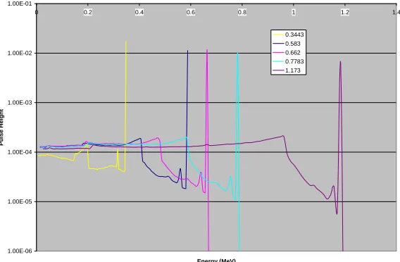
DRF. To see what we have talked about visually, below in Figure 1 is an example of an
MCNP spectrum that is a DRF that is ranged from 0.3443 to 1.173 MeV. This data is not
spread to account for the collection efficiency and imperfections in the detector crystal,
which in this case is Sodium Iodide (NaI). One can easily see the Compton edge sharply.
Other features such as the x-rays from Iodide near the photopeak. The photopeak is one
channel of 1000, which is a purely simulation work. This would correspond to the perfect
1.00E-06 1.00E-05 1.00E-04 1.00E-03 1.00E-02 1.00E-01
0 0.2 0.4 0.6 0.8 1 1.2 1.4
Energy (MeV)
P
u
lse
He
ight
0.3443 0.583 0.662 0.7783 1.173
Figure 1: Part of an MCNP detector unspread response function for Sodium Iodide (NaI)
Others, such as Campbell (1990), have tried to model the parts of the DRF that
are important in the range of interest, in his case low x-ray energies. In one such paper
Campbell added the response of the diodes as part of a (Si)Li drifted detector. All the
components, all the continuants of the semiconductor is calculated separately and then
added up. Some other codes have focused on speed of the generation of DRF. In one such
instance, GADRAS at Sandia National Lab led by Mattingly (Mattingly, 2008), has
produced a very fast DRF code by using a one dimensional approach. The components
are calculated separately and then added up and then spread as in G03, but the Compton
part is the interesting because in 1 dimensional coordinates this response would be unable
to be calculated. This is done by empirical sampling to obtain that part of the response.
The third and the final approach is the semi-empirical approach. This is where one
energy results and processes and then generalizes these results with energy to provide a
continuous model. An example of one of these processes is provided in the code that this
thesis deals with in modeling the detector response functions, G03. This process is a set
of functions that is used for the three photon cross sections in a detector that is of interest.
In this way a search of cross sections in this way is more efficient than a tabular form,
like that found in MCNP. The reason why a semi-empirical approach is chosen and
preferred for some applications is that one does not for example need to model the exact
straggling of the electron. When one considers straggling in electron transport into a
MCNP deck, the time is increased ten fold and the accuracy is also poor because one
does not have the cross sections required for electron transport in single crystals. By
using an empirical relationship that adequately simulates the energy deposited, the code
will be faster, hence more efficient, and much more accurate.
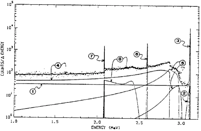
Many authors, including Campbell (1990), devoted much time to producing
specific key features to the detector response functions. Figure 2 is a semiconductor’s
components of the DRF, which is beyond the range of this work, but nevertheless it is
still instructive in showing various components of the DRF. The reason for this is that
although some parts of the DRF for both semiconductors and scintillation detectors have
commonalities, the basic charge collection and detector components differ in that the two
and have entirely different components for the DRF.
This is why on the onset of this code’s development it was proposed by Sood and
Gardner (2004) to use Monte Carlo simulation to obtain certain of the different
them together yields the entire spectrum. This is the central theme of this thesis is that
using a semi-empirical method one can generalize and make slight changes in the code.
This was also accomplished at a great expense to preserving the speed of the code. By
G03’s nature it is simple so in return it is fast, but also easy to manipulate. The trick is in
compiling huge amounts of data and putting it into a semi-empirical model to preserve its
simplicity. An important note is that accuracy suffers. This is due to the fact that, as will
be explained later, G03 runs more computationally efficient by using functional vs. a
tabular acquisition of data. The components added are that of the protective detector
housing, which can constitute around 5% of the total spectrum.
The components are first of all, the most recognizable, the Gaussian standard
deviation of the full energy peak. This applies as well to the entire spectrum. The
exponential tails and the flat continua are also simulated. The flat continuum is produced
because whenever a photoelectron is caused by a photoelectric effect it has an even
probability to deposit its energy. The reason for this is geometry. Let us say you have 1
interaction with two very different effects in the same place lets say at the corner of the
crystal. The first interaction a Compton interaction happens and the electron escapes
without depositing much of the energy, we will call this A. The second one happens at
the same location but the Compton scatter and the electron deposits the full amount of the
energy by evacuating thru the opposite corner, depositing a lot or all of its energy, call it
B. A is the left side of the flat continua and B is the right side. If one really thinks about it
playing all the scenarios or samples in your mind, it makes sense why it is flat. The part
on top is secondary and the bottom part is the tertiary reactions, which represents
possibly many progeny of Compton scatters. It would make since the tertiary reactions
contribution to the spectrum span more of an energy range then the secondary reactions.
Figure 2: Components of the detector response function for Ge Detector (1) the flat
continuum, (2) the exponential tail, (3) the full energy peak, (4) the Compton electron
scattering continuum, (5) a continuum between the Compton electron scattering
continuum and the full energy peak, (6) the single escape peak, (7) the double escape
peak, (8) a small scattering continuum between the single and double escape peaks (Y.
2 CEAR Applications of the DRF
The Center for Engineering Applications of Radioisotopes at North Carolina
University has been investigating DRF for more than three decades. The first few
attempts for CEAR to unlock a DRF were in semiconductor materials. In the late 70’s,
Gardner, Wielopolski, and Verghese (1977) published a paper where the use of the
Monte Carlo method was employed for extending the fundamental parameters of x-rays.
This means they used a semi-empirical approach. The purpose of this was to find
elemental amounts of materials by use of the library least squares method with an energy
dispersive X-ray fluorescence analysis systems. The mathematical models for
components of the response function were in the preliminary stages. In this stage of
computer processor development, huge computers did the same job that a microprocessor
does today. The limitation was computation and it was suggested that experimental
methods should be exploited to speed up response function simulation with many
variations of sample. In CEAR’s second attempt, accomplished by Wielopolski and
Gardner, four spectral features were found in the X-ray energy region. These were the flat
continuum, the exponential tail to the left of each photopeak, the X-ray escape from
Silicon, and the Gaussian photopeak. The models of these equations are shown below in
equations 2.1-2.3. The expressions for each feature are shown, split up, in Figure 3.
)
,
,
'
(
)
(
)
,
,
'
(
E
E
A
1E
F
E
E
C
(2.1))
,
,
'
(
]
'
)
(
exp[
)
(
)
,
,
'
(
E
E
A
2E
A
3E
E
F
E
E
T
(2.2) ] 2 / ) ' ( exp[ ) 2 ( ) , , '
(E E
1/2
1 E E 2
2Where E is the incident photon energy, E’ is the pulse height energy, the A’s are
experimental constants, the F (E”, E, ) are given by (Wielopolski and Gardner, 1979):
" ) , , " ( )
, , ' (
'
dE E E G E
E F
E
(2.4)
And shown explicitly in equation 2.5:
)
(
1
/
2
)
[(
'
)
/
2
,
,
'
(
E
E
erf
E
E
F
(2.5)Figure 3: Illustration of the four features described of a Si(Li) semiconductor detectors
(L. Wielopololski and R. P. Gardner, 1979)
Much work was done in the area of semiconductor materials for CEAR. As
recently as 2008, Fusheng Li has improved the X-ray code using the detector response
function with a GUI interface that provides very useful results or elemental identification
for x-rays. But the scintillation prediction of the DRF is more complex for many reasons.
is that x-ray spectra are at the low keV range, which means that you have a higher
probability of photoelectric absorption. And, in this interaction, one only has to track the
electron until it deposits its energy in the crystal. This is because you do not have to
predict secondary and tertiary interactions in semiconductors. In scintillation detectors,
spectra of up to many MeV are used in experiments, but are rarely used in sub-keV
applications. At these ranges of energy, Compton Scatters have a higher probability of
happening, which is apparent below. It is important to also note that NaI is more
nonlinear than a higher effective Z detector such as LaBr3. Utilizing data from figures 4
through 7, it the belief this is because there is higher probability of Compton Scatter in
the mid-range energies.
Photoelectric Absorption
1.E-08 1.E-07 1.E-06 1.E-05 1.E-04 1.E-03 1.E-02 1.E-01 1.E+00 1.E+01 1.E+02 1.E+03 1.E+04 1.E+05
0.001 0.01 0.1 1 10 100 1000 10000 100000
Energy (MeV)
Cr
oss
se
ct
io
n (
1
/c
m)
NaI LaCl BGO LSO LaBr
Figure 4: Photoelectric Effect Cross Sections for many types of detectors.
Photoelectric Absorption
1.E+00 1.E+01 1.E+02 1.E+03 1.E+04 1.E+05
1.E-03 1.E-02 1.E-01 1.E+00
Energy (MeV)
C
ro
ss
s
ec
tio
n
(
1
/c
m
)
NaI LaCl BGO LSO LaBr
Figure 5: Photoelectric Effect Cross Sections Zoomed in. Element/Compound/Mixture
Selection, from NIST XCOM website
Compton
1.E-05 1.E-04 1.E-03 1.E-02 1.E-01 1.E+00
0.001 0.01 0.1 1 10 100 1000 10000 100000
Energy (MeV)
Cr
o
ss secti
o
n
(1
/c
m)
NaI LaCl BGO LSO LaBr
Figure 6: Compton (Incoherent) Scattering Cross Sections for many types of detectors.
Pair Production
1.E-04 1.E-03 1.E-02 1.E-01 1.E+00
1 10 100 1000 10000 100000
Energy (MeV)
C
ro
ss se
cti
o
n
(1
/c
m)
NaI LaCl BGO LSO LaBr
Figure 7: Pair Production Cross Sections for many types of detectors.
To further complicate matters, there is also is a higher probability of pair
production for the range of energies for which scintillation detectors are applicable. So,
annihilation photons must be tracked as well. In a code like MCNP, complicated electron
models are employed to get the pulse height for a detector volume. This can multiply the
computation time more than 10 fold.
CEAR started studies in the early 1990’s to tackle this difficult problem of the
scintillation DRF. In the code named DRFNCS, a semi-empirical approach was
employed to calculate detector responses for many energies of photons incident on the
crystal. This code is the very beginnings of G03, which is the code to which the
improvements are to be made. Much of the geometry tracking done in the present G03 is
used exactly the same way it was in the 1990’s, with some optimizations for time. Berger
and Seltzer (1972) cited that the addition of the Bremsstrahlung radiation contribution to
code, the electron had a simple range relationship that is shown in equation 2.7. This
enables the code to run very fast.
) ln
(b c E
e
aE R
(2.6)
The code also used basic photon interactions such as pair production, Compton
Scattering, and photoelectric effect, and excluded unnecessary interactions such as
Rayleigh scattering. The photoelectric effect assumes isotropic scattering for the
photoelectron. The Compton Scattering is treated with the standard Klein-Nishina
formula and the Kahn rejection technique (Kahn, 1954) was applied to select an energy
and subsequent scatter direction. The pair production interaction assumed an isotropic
distribution of the electron and positron with a minimum angle m, shown below as:
h c
mo
m
2
(2.7)
This study yielded some interesting and accurate data. The problem, when comparing it
to the experiment, is that there are large variances in the valley region as well as
discrepancies in the Compton Continuum in the present G03 that will be shown later.
3 Inherent Problems with G03 and Motivation for Its Modification
G03 is a very useful tool for calculating response functions for some detectors.
The Center for Engineering Applications of Radioisotopes, CEAR, is looking to use these
response functions to produce radioisotope (or elemental) library spectra to help with
Homeland Security in order to make the inspection of cargos at seaports and at our
borders more efficient and more accurate. In order to convolve simulated radioisotope
photon and neutron spectra of different yields and types, one must look at all parts of the
spectra. In addition, the response function could be applicable in concert with the
elemental analysis of many composite compounds between the source and detector,
especially when considering high resolution detectors such as lanthanum and germanium
detectors.
However, there are some developments G03 has to hurtle. The analyses of G03, in
its current phase, needs to be accomplished in all parts of the spectra and accuracy are
important. Simulated spectra that are orders of magnitude differentiated by use with and
without the protective can around it, may lead to as much as 0.001- 0.0001% difference
in the normalized intensity of the photopeak. These are things that must be observed and
changed regarding this approach to the detector response function.
Any Monte Carlo code will never have a perfect representation of a detector
response function for any type of detector. This is due to the fact that every
detector is different: from the differing compositions of the cans being used, to
effects from crystals grown that have not yet been actually modeled at this time,
The detector is a bare crystal. Avneet Sood’s thesis (2000) has stated that the
addition of the front face of the can would contribute to the improvement on yield
in the valley region. It is also evident, which will be shown later, that the side
detector crystal covering contributes to slight fluctuations in the Compton
Continuum energy range. There is also a possibility that the PMT, at high incident
photon energies, can affect the spectra. CEAR provides new features of the
detector response function and, in doing the modification of G03, will provide
more accuracy. One of the objectives in this research is to prove that, although
these effects may seem small, they are an important part of the DRF because they
are large enough to affect the accuracy of the inverse problem.
G03 cannot simulate the complex geometry involved in the DRF where the
detector source is not on a major axis of the detector. But, in the detector-source
configurations that are different, the use of different distances would be
advantageous. This is due to the fact that a 3rd variable for elemental composition
is now available. It would also be useful in the area of oil well logging to simulate
the detector-source configuration on the side of the detector.
The non-linearity and the flat continua can be very easily put into the spectra of
G03. CEAR has already demonstrated this (Gardner and Sood, 2004). The flat
continua can be thought of as a sort of geometry factor. The flat continuum is
easily explained by its flatness, and is shown in the last figure of the first chapter
of this thesis. The flat continuum is caused by the escape of electrons from the
or the Compton Scattering process, there are finite probabilities of distance out of
the detector. Therefore, the effect gives an approximately flat shape because the
electrons behave in an approximately constant dx dE
relationship. This relationship
dictates that the electron gradually loses its energy as a function of distance
traveled. For example, the right side of the flat continua is demonstrated when a
photoelectric effect happens near the corner and the photoelectron’s trajectory
takes it towards the opposite corner. And conversely, on the left site of the
continua, when a photoelectric effect happens, and it is near the corner of the
detector, the electron’s trajectory is the smallest possible distance out of the
detector, so it deposits very little energy. Straggling effects are the result of a
process in which the electron trajectory has a tendency to be erratic. In actuality,
electrons are either absorbed or scattered, which G03 is not considering. In the
last chapter, the semi-empirical relationship that describes the electron transport is
not based on this. This is a way to simplify and spend less money on computer
calculation times because the complex electron transport that is employed in
MCNP5 takes a factor of ten more times than when electron transport is not
considered.
Parts of the code were written in an f77 FORTRAN context; this is to be changed
in all subroutines and main processes. This is done for practical efficiently
purposes.
A possible upgrade to MCNP search for cross section data, which is done in
photon cross sections, as well as the total of the three. This cross section protocol
will be benchmarked against MCNP’s cross section procedure. This can be easily
explained as an analysis of functional vs. tabular.
More modifications and notes to those modifications will be added to the code to
benefit future code users.
Does not include the natural radioactivity that some of the elements used in
detectors have, such as lanthanum detectors. Note: this is a low energy, low yield
effect as demonstrated in Figure 8. complements of (INL, Hartwell, personal
correspondence supplied by Harp).
0.001 0.01 0.1 1
0 200 400 600 800 1000 1200 1400 1600
Energy (keV)
Normal
iz
ed
co
un
ts
Figure 8: Background of radioactivity coming from the lanthanum part of La3Br
G03 is limited to only simulating NaI, and no other types of detectors. No high
resolution scintillation detector data is available at the present time, and at high
energy This is due to the fact that higher order interactions need to be added like
Detector size, at present, has been limited to 3 X 3 and some 6 X 6 simulations.
4 MCNP Simulation of Can Phenomena
At this time, we decided to run an investigation of what exactly the detector can
contribute to the spectrum. The source was used isotropically but. in order to save time.
the tightest geometry was employed. The MCNP universe was shaped in a cylinder with
the diameter just larger than a typical 3x3 NaI detector and as long as the length of the
detector plus 10 centimeters. The extra 10 centimeters is used for the source that is
aligned on axis with the detector. The first simulations were with no detector protective
can (WOC), with the front of the can only (WC), and with the can on the detector
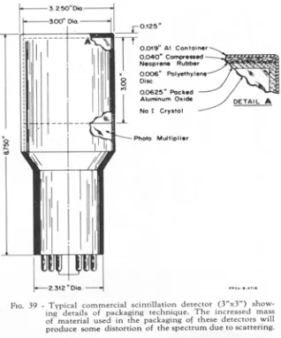
(WWC). The detector specs where given in Heath and are shown below in figure 9. As
shown below, the front of the can has four layers, while the side of the can has only two
and is 36% less thick than the front. It is important to note that the higher atomic Z
number, meaning more protons are present, the higher the probability of interaction with
the side of the can which is important when Neoprene Rubber is present. It is composed
of a little hydrogen, with 52% by weight Carbon, and very near 40% by weight Chlorine,
Figure 9: Heath can schematic. (1964)
The three simulations were run in order to find what the detectors affect in the can
that has been stated earlier in Sood and compensate for the difference in the valley
region. Is it the electrons of photons in the front of the can? Or maybe other parts of the
spectrum’s variability can be attributed to the can on the side from photons bouncing
back in from a Compton? Or electrons staggering in and out of the can into the crystal. At
this point, only a surface tally was preformed between the front face and the front of the
crystal. This is because it was hypothesized that this was the dominant effect that was
affirmed the in Sood Thesis (2000). The pulse height tally also runs for the three
simulations. Also later in order to be sure an electron current tally was employed at the
can crystal interface. All the detectors were run at 27 different energies from 0.01 to 10
MeV. This is cataloged as an unspread MCNP detector response function.
These results show that it is indeed the front of the can that contributes to the
continuum in the Compton range is present. The “edge” is in the same energy for all of
the different simulations for different detectors, and at different energies. One way to
explain it is to say that the detector can side provides a specific backscatter into the
continuum were this energy is located.
Into the investigation of the input file, the photopeak was found as a function of
energy to be as much as 94% of the total spectrum, which is shown below in Figure 12.
This could explain the valley region seen in Figure 13. This is a spectrum of the
photons actually striking the crystal, after they have been attenuated throughout the can.
Figure 14 shows further interesting results. The graph states that many photons are
attenuating through the can and spreading throughout the spectrum. This causes a
sizeable difference in the valley region, which can be explained as many different
photopeaks in the valley region, due to Compton Scatters. This is shown in Figure 13 at
the five low energies, with same the 3x3 NaI detector. We also obtained the electrons
from the three basic interactions, which will affect the spectrum. This is shown below in
94.0% 94.5% 95.0% 95.5% 96.0% 96.5% 97.0% 97.5% 98.0%
0 1 2 3 4 5 6 7 8 9 10
Energy (MeV) P e rc en ta g e o f in cid e n t o n c ry s ta l th a t is in c id e n t at th e c a n o f s a m e en er g y
Figure 10: Percentage of photons going through the front of the detector can that are not
being attenuated for Heath 3x3.
1.E-06 1.E-05 1.E-04 1.E-03 1.E-02 1.E-01 1.E+00
0 0.2 0.4 0.6 0.8 1 1.2
Energy (M eV)
S u rf a c e C u rre n t f o r P h o to n s 0.344 0.583 0.662 0.778 1.173
1.E-07 1.E-06 1.E-05
0 0.2 0.4 0.6 0.8 1 1.2
Energy (MeV)
Su
rf
ace
C
u
rr
ent
f
o
r Elect
ro
ns
0.344 0.583 0.662 0.778 1.173
Figure 12: Electron spectrum incident on the crystal after being attenuated thought the
can.
The analysis of some of the MCNP output yielded showed interesting results. It showed
that the side of the housing, or can, might actually be caused not from the front of the can
0.E+00 1.E+06 2.E+06 3.E+06 4.E+06 5.E+06 6.E+06 7.E+06 8.E+06
0 1 2 3 4 5 6 7 8 9 10
Energy (MeV) Co mp to n i n ter a c ti o n s wwc wc woc
Figure 13: Compton interactions with the whole protective can (wwc), without the can
(woc), and with just the front face (wc).
-5.0E+06 0.0E+00 5.0E+06 1.0E+07 1.5E+07 2.0E+07 2.5E+07
0 1 2 3 4 5 6 7 8 9 10
Energy (MeV) e lec tr on auger i n te ra ct ions wwc wc woc
Figure 14: Auger electron with the whole protective can (wwc), without the can (woc),
and with just the front face (wc).
The results are shown below in figures 15-17 for NaI, BGO, and La3Br detectors
which were run for comparison. The difference between the simulations of the one with
the front of can and the whole can show the effects can be shown in the Compton
simulation assumes a perfect crystal with no defects. The detector’s imperfection in non-
unity ratio to energy deposited to charge collection is the non linearity and a function of
peak shift and the non linearity. Since it is a perfect detector, one can observe the X-rays
from the higher Z constituents of the detector crystal.
1.E-05 1.E-04 1.E-03 1.E-02 1.E-01
0 0.1 0.2 0.3 0.4 0.5 0.6 0.7
Energy (MeV)
Pu
ls
e
He
ig
h
t T
a
lly
in
MCNP (f8
)
woc wc wwc
Figure 15: NaI Unspread spectra.
1.E-07 1.E-06 1.E-05 1.E-04 1.E-03 1.E-02 1.E-01
0 0.1 0.2 0.3 0.4 0.5 0.6 0.7
Energy (MeV)
P
u
lse H
e
ight
Without can With Front Face of Can With Al of the Can
1.E-07 1.E-06 1.E-05 1.E-04 1.E-03 1.E-02 1.E-01
0 0.1 0.2 0.3 0.4 0.5 0.6 0.7
Energy (MeV)
P
u
lse H
e
ig
ht
Bsre cyrstal
With the front of the can, no sides With the whole can over the detector
Figure 17: LaBr Unspread spectra.
This data represents a preliminary investigation into how the can affects the spectra.
Now, if we are to implement it into G03, some things need to be done, in order to fully
add the contribution to the can:
1. The spectra that needs to be interpolated needs to have the same number of
channels regardless of energy. This was not done earlier; instead the simulations
had 256 channels across the whole energy range, which was different depending
on the energy studied. For these later simulations, there were 1002 channels
spanned from 0 to 10 MeV
2. The contribution to the outside of the can needs to be documented for both
electrons and photons. The reason for this documentation is clearly illustrated in
figures 15-17. The spectrum, with only the front face of the can, was lower in the
Compton Continuum than the simulations for the whole can for all three different
Compton Continuum where there is a “backwards” continuum. It is at the same
energy for all three different types of detectors. Effectively, this means that this is
a direct function of the composition of the can. G03 is based on the Heath data,
and other detectors might not be represented here perfectly. It is important to note
that this is an approximation, acknowledging that some photons can scatter out,
and then back inside.
3. Investigate the possible contribution of the PMT-detector interface to the DRF.
Some of these goals that were put in place for MCNP were hard while others were easy.
The first goal was easiest because all that was necessary was change a couple lines of
code. Number two was relatively easy, but number three took a great deal of effort. The
problem is that MCNP does not have surface treatment explicitly for a curved surface like
it does for the flat surface. This is because the flat surface can easily be divided up into
out or in the Cosine being positive or negative, which is the command in MNCP. To
define a Cosine angle for a curved surface is not done in MCNP. So, with some help from
my colleges, a strategy was employed to get the flux of the outer can. Two decks were
run, one with and one without the detector can, rather than the three described earlier. A
surface flux tally was obtained from these two. And then the tally of the one without the
can was subtracted from the one with the can. Again, it is important to note that this is an
approximation. This is due to the fact that there are some interactions where a photon can
bounce back and forth between the crystal and the can, and affect the accuracy of this
detector can. This was done in order to obtain the per source particle representation of the
current coming back into the can for the photons. The results of this are shown below in
figures 18 and 19, for the lower energy runs. And, in figures 20 and 21, are the results of
the attenuated current that strikes the crystal from the front.
1.00E-07 1.00E-06 1.00E-05 1.00E-04
0 0.1 0.2 0.3 0.4 0.5 0.6 0.7 0.8 0.9 1
Energy (MeV) C u rr e n t o f p h o to n s aft er th ey h a v e b e at te nu at ed b y ca n (1 / so ur c e p a rt ic le ) 0.3443 0.583 0.662 0.778 1.332
Figure 18: Electron spectrum bouncing back into the detector from the side.
1.00E-07 1.00E-06 1.00E-05 1.00E-04 1.00E-03 1.00E-02 1.00E-01
0 0.2 0.4 0.6 0.8 1 1.2
Energy (MeV) C u rrent of pho ton s a ft e r t h ey ha ve b e a tt e nua ted by ca n ( 1 / so urce part ic le ) 0.3443 0.583 0.662 0.778 1.332
1.E-06 1.E-05
0 0.2 0.4 0.6 0.8 1
Energy (MeV) C u rr e nt of elec tr ons after they h a ve
be attenuated by
can (1 / sour ce par ticle ) 0.3443 0.583 0.662 0.778 1.332
Figure 20: Electron spectrum incident on the crystal after being attenuated thought the
can. 1.00E-07 1.00E-06 1.00E-05 1.00E-04 1.00E-03 1.00E-02 1.00E-01
0 0.2 0.4 0.6 0.8 1 1.2
Energy (MeV) Cur re nt of pho tons a ft e r t h e y h a v e be a tt e nua te d by c a n ( 1 / s ourc e pa rt ic le ) 0.3443 0.583 0.662 0.778 1.332
Figure 21: Photon spectrum incident on the crystal after being attenuated thought the can
In addition to comparing G03 with Heath, CEAR wanted to benchmark against
other types of detectors. The detectors that were considered included St. Gobain’s 2x2
NaI, BGO, and LSO. These were all wrapped with Teflon in order to keep the important
the crystal. Then, everything is surrounded by Aluminum. Also included is a plastic box
scintillator that is 2”x12”x12” in volume, which is needed for the DRF for CEARCPG.
The theory is that coincidence counting would be more efficient for a detector that has a
massive volume. All the detectors were simulated for 7 energies up to 2.614 MeV, 10 cm
from the front of the detector and all the tallies obtain basically the same thing: the
photons coming back into the detector. For the box detector, only the whole can needed
to be simulated because we do not have the curved surface problem that we had for
cylindrical detectors. The Homeland Security detector is a 16”x4”x2” NaI detector from
St. Gobain and shown in figure 20. The box detectors were simulated on the widest
surface area side, which is the way it is employed in the field to maximize efficiency. The
big difference is that electrons were not simulated because the low yield and hence
negligible contribution to the response. The cylindrical detectors, shown quantitatively in
Figure 21, are all assumed to be the front.
Figure 23: Typical Detector Housing for all produced 2x2 Cylindrical Detector
5 Implantation of Simulated Phenomena into G03
The primary purpose of this project is to implant all of these effects into the
existing G03 code and then see if the spectra would be more representative of what
happens in the can. The biggest contribution comes from the photons that go through the
front of the can. This part is essentially a detector response function within itself. This is
because what is actually hitting the crystal is several monoenergetic photons hitting the
crystal, at different yields, and adding those responses to get the spectra that should be
seen in the experiment.
To accomplish this feat, it is done very similarly to that described above. From
Chapter 4 we have the spectra per source particle entering the front of the can for 20
monoenergetic photons. With this data we can 3 dimensionally obtain the spectra for any
energies between 0.01and 10 MeV. This 3-D universe has the 3 axis of: (1) Energy of
incident photons on can-E, (2) Attenuated photon energy- E’, and (3) Tally as function of
f(E,E’). In order to simplify the use of three 3-d full interpolation the functions of
f[EN,f(E,Tal)], which is a fancy way of saying for every incident energy on the can there
is a spectrum that can be represented in a piecewise graph. The point in which G03 calls
its energy which is monogenetic in each spectrum, which is the inter loop of G03, it goes
through this interpolation.
Another way to keep G03 moving faster is to do a post-processing step instead.
figure 24 below is the photon spectra (normalized to unity) after it passes through the
protective can for one of those energies, cesium energy in this case. The plot can be seen
crystal. The reason why it is normalized is when the can spectra hits the crystal all the
appropriate weights for the geometry factor have been accounted for in G03. Otherwise,
the photon flux incident of the can/crystal interface. It looks like the photopeak energy is
unity, but it looks close to it on a semi-log graph. For Cs we have 95.1% uncollided flux.
The rest is just 4.9% of the spectra but it is deposited throughout the spectra. To add the
can contribution in a simple way is to treat each one of these points as the spectra of
certain abundance. So then, the unspread, non-linear library with the light yield included
is multiplied channel-by-channel and simultaneously added together to obtain the total
spectra. The unspread data needed to be obtained, and is shown in figure 25. The result of
this is spread so instead of many peaks, it will smooth out and have a flat continuum, due
to majority of the continuants, again 95.1%. Then the spread is then applied which
changes the bums from all those monoenergetic spectra will sooth out.
Cs Energy (0.662 MeV) Spectrum of Photons After being attnuated by the can
1.E-06 1.E-05 1.E-04 1.E-03 1.E-02 1.E-01 1.E+00
0 0.1 0.2 0.3 0.4 0.5 0.6 0.7
Energy (MeV)
No
rm
alized
ph
o
to
n
s
h
itt
in
g
th
e cr
yst
al
Figure 24: Cesium spectra point wise after attenuated through the front of the protective
1 10 100 1000 10000 100000
0 0.1 0.2 0.3 0.4 0.5 0.6 0.7 0.8
Energy (MeV)
Co
u
n
ts
Figure 25: Unspread spectra for Cesium Unshifted spectra from G03
The same can be accomplished with the side of the can contribution, which is
responsible for the backwards continuum, previously shown in chapter 4. This is the
difference between the detector with its whole protective housing, the second with the
front face of the cylinder being covered, and the third being with the bare crystal.
The way that the photon contribution from the side of the can. Discussed earlier,
this happens when an interaction brings the incident photon back into the can. The
process of deduction is Compton, Pair Production from the anti-annihilation photon, and
secondary interactions. In order to conserve yield the per-source particle the spectra will
be maintained, with no normalizing. Let us say for instance that there is a G03 run done
with 70,000 particles per spectrum. The spectrum of Indium would have the addition of
the photon side run in MCNP. This is done in a per source particle per source particle
addition to the spectrum. The fraction of the spectrum addition per source particle is
earlier mention f8 tally. It is important to mention that the first or 0 channel or 0 energy
probability in the MCNP will be unity minus the total of the spectrum below. In this way
the per source particle will be preserved. If a G03 run is to run at the intermit spectrum of
0.662 MeV, which is on of the MCNP run detailed in chapter 4 of this work, and had
10,000 histories the addition from the electrons would be the spectrum in figure 26 times
10,000 for each channel. Now one can see how the backwards continuum is form as an
addition to the spectra.
1.E-07 1.E-06 1.E-05 1.E-04 1.E-03
0 0.1 0.2 0.3 0.4 0.5 0.6 0.7
Energy (MeV)
Per
sou
rc
e par
ti
cl
e for pho
tons
fl
ux
o
n
the s
ide of ca
n
Figure 26: Per source particle of photons coming back into the crystal from the side.
Therefore, this work generalizes a DRF for any size type and shape, with a
particular attention to contribution of the can. This was stated earlier apart of the detector
response function because it is apart of the detector. To that goal a treatment has to be
devised to address the variation of detector sizes first. A method was devised and
Gaussian parameters available in G03 are for 3x3, 3x6, and 6x6 detectors. The
parameters that dictate the equation for the spreading is:
b
aE
(5.1)
The parameters that are stated in Gardner and Sood are:
Table 1: Gaussian Spreading Parameters from the original G03
3x3 3x6 6x6
a 0.0307 0.04009 0.02609
b 0.65934 0.36064 0.6027
Were differential operator come into play, that there is an assumption that there is
correlation between the Gaussian parameters and physical dimensions such as volume,
surface area, length, and radius. There are 3 different approaches that the author took to
quantify this phenomenon:
1. Differential Volume:
nxn x x x x nxn V V V ab ab
ab) ( ) ( ) *
( 2 2 6 6 2 2 6 6
(5.2)
2. Differential Surface Area:
nxn x x x x nxn SA SA SA ab ab
ab) ( ) ( ) *
( 2 2 6 6 2 2 6 6
3. Differential Fundamental Dimensions: nxn x x x x nxn x x x x nxn L L L ab ab D D D ab ab
ab) ( ) ( ) * ( ) ( ) *
( 2 2 6 6 2 2 6 6 2 2 6 6 2 2 6 6
(5.4)
where D is the diameter of the detector, L is the length, SA is the surface area normal to
the surface at a set distance, and V is for Volume. The notation (ab) stands for either a or
b as appropriate for a certain detector of equal diameter and length.
In order to further generalize a DRF code it was conceived that a box needed to be
simulated. For practical purposes right now a box plastic scintillator and the St. Gobain
Box detector is going to be benchmarked. The added flexibility was added to give any
dimension at first at any distance normal to any surface. Then later the geometry option
was added so that the source can be at any point or orientation, since they are mutually
exclusive. Both programs or subroutines calculate the distance that a ray passes though a
detector in a random fashion based solely on the random cosine angle. First, G03
calculates this distance of this ray for every particle initiated. Then the total cross section
and type of interaction for that matter is calculated. Based on these two numbers a
weight, and random interaction site is calculated. This is the reason why G03 is faster
than MCNP in some ways. MCNP has to make a random choice at every surface were
conversely, G03 is simple math and geometry simplification that is quite accurate. The
necessary weights are calculated to the forcing of interaction into G03. So by its nature
biasing is done so every particle hits the detector regardless of distance and every particle
After that interaction, G03 calls another subroutine that calculates based on where the
interaction happens moves the direction of the angle cosine, hence its trajectory, to the
longest distance out of that detector. It does this based on the fact that in the cosine angles
can be manipulated, in the plus minus sense, to have 6 variations in direction. This
subroutine, called Travel, was developed by Douglas Peplow (Peplow, Gardner and
Verghese, 1993) for the cylindrical case calculated the distance between the interaction
site and the three surfaces, the two top discs and the periphery of the crystal. Then Travel
subroutine forces the interaction to go to farthest distance plane, and calculated the
crucial weights.
In the sprit of generalizing this code different materials need to be considered. As
stated before the parameters are easy to manipulate. It is just finding the right place in the
code, actually most of the time in the subroutines, to change it to represent the response
for different materials. Electron Range relationship for other materials:
2 1
1 2
2 1
A A R
R
(5.5)
To accommodate the change of Bremsstrahlung in materials G03 weighting was shifted
based on the actual Bremsstrahlung that NaI would cause. The ratio in the yields, like the
ratio of range, are calculated and then multiplied in the weight due to the Z dependence:
ZT ZT Y
* 10 * 6 1
* 10 * 6
4 4
(5.6)
Were Z and A is effective Z and A, and respectively the effective number of protons or
atomic weight, of detector crystal material. T is energy, is density, and R is the Range
part were this is needed is the calculation of the flat continuum. This is because the
density is imbedded into the cross sections of every material, which needs to be changed.
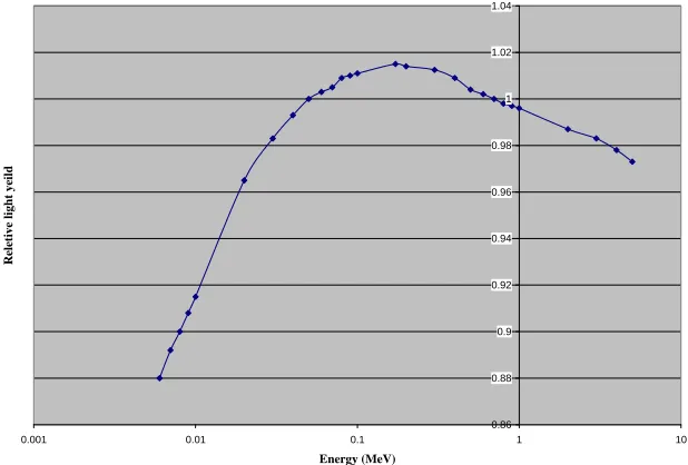
The nonlinearity caused by the light yield, or electron collection efficacy, was added.
This dramatically affects the actual behavior of the response. The relative light yield as a
function is shown in Valentine et. al for NaI, LSO, and BGO detectors is shown below in
Figure 27, and the light yield shown in Figure 28 is for LaBr.
Figure 27: Light yield for various detectors. (Mengesha, Taulbee, Rooney, and Valintine,
0.86 0.88 0.9 0.92 0.94 0.96 0.98 1 1.02 1.04
0.001 0.01 0.1 1 10
Energy (MeV)
R
ele
tive
light
ye
il
d
Figure 28: Light Yield for La3Br
The first thing that was done to improve the time is the conversion of G03 from
FORTRAN77 to FORTRAN99. The cross section treatments are a perfect example of
this. One can do it like in G03, where the cross section is obtained in a functional form,
but accuracy is not as good as it should be. Another approach to this problem is a tabular
one like in MCNP. Unfortunately for MNCP time is sacrificed for accuracy, due to the
fact of how tabular data is processed. Any searches through data no matter how proficient
it has to first go through searching for the number of two energies that the energy in
question that need to be interpolated, then interpolate. It has to interpolate because the
probability of hitting a specific tabular integer for double precession is very low. In G03
the functional form eliminates the need of searches and secondary equations. If one puts
Scattering, and Pair Production. In turn, the total cross section which is the parameter that
6 Results
6.1 Overall Statement of Detector Parameters and Preliminary Results
The results are from the cylindrical can compositions are shown in Chapter 2. The
results are from the box detector compositions are shown in Chapter 4. The
source-to-detector distance is 10 cm from the front of the can. Also different source-to-detector materials are
shown. The variations that are not shown, but are also available are from the incident
photons on the front and from the side, as well as electrons from the front and side. Also
available but not shown is the case where the photon flux is going out the back hitting the
PMT. The Box detectors were simulated with the source normal to the largest surface
area and 10 cm away.
1.E-07 1.E-06 1.E-05 1.E-04 1.E-03 1.E-02 1.E-01 1.E+00
0 0.1 0.2 0.3 0.4 0.5 0.6 0.7 0.8
Energy (MeV)
C
o
u
n
ts
/(
To
ta
l Co
unt
s)
with whole can without can with front face
1.E-07 1.E-06 1.E-05 1.E-04 1.E-03 1.E-02 1.E-01
0 0.5 1 1.5 2 2.5 3
Energy (MeV)
P
u
lse Hei
g
h
t
3x3 6x6 2x2
Figure 30: Heath can for different size NaI detectors Without Detector Housing for 2.614 MeV
1.E-06 1.E-05 1.E-04 1.E-03 1.E-02 1.E-01
0 0.5 1 1.5 2 2.5 3
Energy (MeV)
Pu
lse Heigh
t
3x3 6x6 2x2
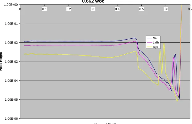
0.662 woc
1.00E-06 1.00E-05 1.00E-04 1.00E-03 1.00E-02 1.00E-01 1.00E+00
0 0.1 0.2 0.3 0.4 0.5 0.6 0.7
Energy (MeV)
Pu
lse
He
ig
h
t
NaI LaBr Bgo
Figure 32: Without Heath can, different types of 3x3 Detectors for 0.662 MeV
0.662 wwc
1.E-06 1.E-05 1.E-04 1.E-03 1.E-02 1.E-01 1.E+00
0 0.1 0.2 0.3 0.4 0.5 0.6 0.7
Energy (MeV)
P
u
lse
he
ig
ht
pe
r So
ur
ce
Pa
rt
ic
le
NaI LaBr Bgo
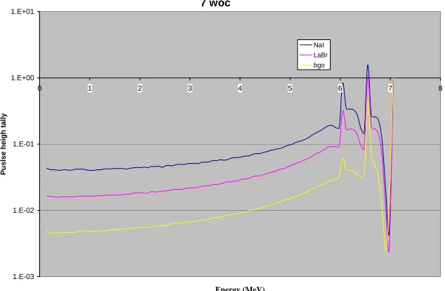
7 woc
1.E-03 1.E-02 1.E-01 1.E+00 1.E+01
0 1 2 3 4 5 6 7 8
Energy (MeV)
P
u
slse
heigh
tally
NaI LaBr bgo
Figure 34: Without Heath can, different types of 3x3 Detectors for 7 MeV
7 wwc
1.E-03 1.E-02 1.E-01 1.E+00 1.E+01
0 1 2 3 4 5 6 7 8
Energy (MeV)
Tal
ly
NaI LaBr bgo
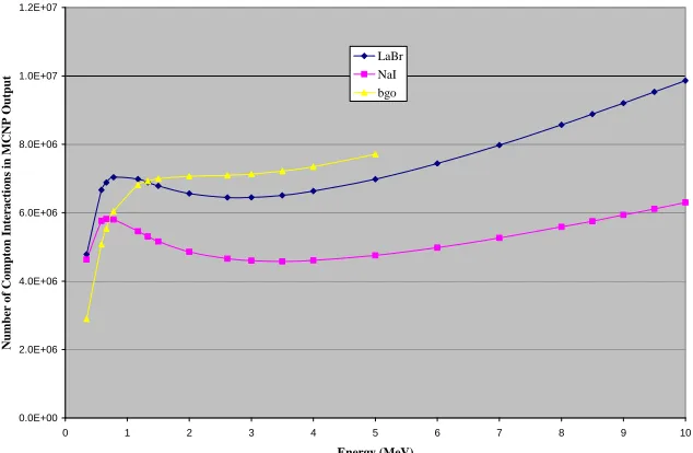
0.0E+00 2.0E+06 4.0E+06 6.0E+06 8.0E+06 1.0E+07 1.2E+07
0 1 2 3 4 5 6 7 8 9 10
Energy (MeV) Nu mb er o f Co mp to n I n teracti o n s in MCN P O u tp u t LaBr NaI bgo
Figure 36: Compton interactions for various detector types, and without the protective can. 0.0E+00 2.0E+06 4.0E+06 6.0E+06 8.0E+06 1.0E+07 1.2E+07
0 1 2 3 4 5 6 7 8 9 10
Energy (MeV) N u m b er of C o mp ton In teract ion s in MC N P Ou tp u t LaBr NaI bgo LaCl
1.E-07 1.E-06 1.E-05 1.E-04 1.E-03 1.E-02 1.E-01
0 0.1 0.2 0.3 0.4 0.5 0.6 0.7
Energy (MeV)
P
u
ls
e H
eig
ht
woc wc wwc
Figure 38: 3x3 LaBr detectors at 0.662 incident energy 256 channels with Heath can
1.E-07 1.E-06 1.E-05 1.E-04 1.E-03 1.E-02 1.E-01
0 0.2 0.4 0.6 0.8 1 1.2 1.4
Energy (MeV)
Puls
e Height
woc wc wwc