New Techniques for High-Dimensional and Complex Data Analysis Based on Weighted Learning.

(1)

ABSTRACT

SHIN, SEUNG JUN. New Techniques for High-Dimensional and Complex Data Analysis Based on Weighted Learning. (Under the direction of Yichao Wu and Hao Helen Zhang.)

We develop new statistical tools for high-dimensional and complex data which have

been very common in many applications. The thesis consists of four topics and a common

thread which links all the inter-related topics is weighted learning.

In the ﬁrst two chapters, we establish the joint piecewise linearity of two popular

kernel machines, the weighted support vector machine (WSVM) and the kernel quantile

regression (KQR), which possess additional parameters besides the regularization

param-eter, a weight parameter and a quantile paramparam-eter, respectively. In Chapter two, joint

piecewise linearity of the WSVM solution is established and then an associated algorithm which eﬃciently computes entire solution surfaces of the WSVM is proposed. In Chapter

three, a piecewise linear conditional survival function estimator is proposed based on the

two-dimensional solution surfaces of the censored kernel quantile regression which can be

viewed as a special case of the weighted KQR.

In the remaining two chapters, we study suﬃcient dimension reduction (SDR) in

bi-nary classiﬁcation. While SDR has been extensively explored in the context of regression

with continuous response, SDR in binary classiﬁcation where most of existing SDR

meth-ods suﬀer has not been thoroughly researched. We propose two novel SDR estimation

methods in the context of binary classiﬁcation. In Chapter four, a probability-enhanced SDR scheme is proposed. The key idea is to slice data based on the conditional class

probability rather than the binary response. Such a probability-based slicing can be

con-veniently done by solving a sequence of WSVMs. In Chapter ﬁve, we develop a weighted

principal support vector machine (WPSVM) for SDR in binary classiﬁcation by

extend-ing the idea of the principal support vector machine (PSVM) recently developed by Li

et al. (2011) in the context of regression. The proposed WPSVM successfully achieves

SDR with binary responses and can handle both linear and nonlinear SDR in a uniﬁed

(2)

(3)

New Techniques for High-Dimensional and Complex Data Analysis Based on Weighted Learning

by Seung Jun Shin

A dissertation submitted to the Graduate Faculty of North Carolina State University

in partial fulﬁllment of the requirements for the Degree of

Doctor of Philosophy

Statistics

Raleigh, North Carolina

2013

APPROVED BY:

Leonardo A. Stefanski Hua Zhou

Yichao Wu

Co-chair of Advisory Committee

Hao Helen Zhang

(4)

DEDICATION

(5)

BIOGRAPHY

Seung Jun Shin is from a beautiful city of Busan, the largest costal city in South Korea.

After graduate high school in 2000, he left his hometown to attend Korea University in

Seoul, the capital of South Korea where he earned a Bachelor degree in statistics with

economics.

He then joined Master program at Korea university and continued to study more

advanced topics in statistics. Under the direction of Dr. Myoungshic Jhun, Seung Jun was involved in three projects which mainly focussed on bootstrap and nonparametric

function estimation. After the completion of Master degree, he worked as a research

as-sociate at Institute of Statistics, Korea University and a part time lecturer at Sookmyung

Women’s University in South Korea.

In 2008, Seung Jun left Korea to pursue Ph.D. degree in statistics at North Carolina

State University in Raleigh, North Carolina. He has been motivated much of his research

in high-dimensional data analysis. His general research interest includes kernel machine,

dimension reduction, model selection, nonparametric function estimation and bootstrap.

Toward his PhD degree, he has been developed new techniques for high-dimensional and complex data analysis based on weighted learning under the direction of Drs. Yichao Wu

(6)

ACKNOWLEDGEMENTS

There are many people who have helped and guided me through my academic journey.

I would like to take this opportunity to express my gratitude to a few people while

acknowledging that many more people deserve praise.

I would like to express my deep and sincere appreciation to my advisors Drs. Yichao

Wu and Hao Helen Zhang for their generosity and patience for me. Thanks for their full

emotional and ﬁnancial support, I could entirely focus on my academic work during my PhD research. Their profound insight into statistics and professionalism let me explore a

variety of areas in modern statistics which will be valuable asset for my future academic

achievement. It was my great fortune to have them as my academic mentors.

I wish to thank all the faculties and staﬀs in our department. My appreciation should

go to Drs. Len Stefanski and Hua Zhou for joining my committee and suggesting

con-structive comments and suggestions that led to signiﬁcant improvement of my dissertation

research. I want to thank both current and previous directors of the graduate program

in the department during my years in North Carolina State University, Drs. Sujit Ghosh

and Jacqueline Hueghes-Oliver for generously answering all the questions that I had have. Especially, I would like to thank Dr. Sujit Ghosh for suggesting an excellent idea during

his course, Bayesian Biostatistics and spending additional time to write a paper with

me. I am also appreciated of all the enthusiastic teachers of the courses that I had taken

in graduate school. I particularly thank the two wonderful teachers for their excellence

in teaching, Dr. Subhashis Ghoshal of asymptotic statistics and Dr. Butch Tsiatis of

semiparametric inference and missing data.

I also want to express my gratitude to people who support me in my home country,

Korea. My deep appreciation should ﬁrstly go to Dr. Myuongshic Jhun who led me to

the world of statistics and has always given me full support in many ways. Although I cannot acknowledge individually by names, I am very thankful to all the faculty members

in statistics department at Korea University. It was great to start my academic life with

such great mentors. My special thanks also goes to my friends in Korea. Memory

of wonderful days with them has always refreshed me whenever I have had hard time

(7)

(8)

LIST OF TABLES

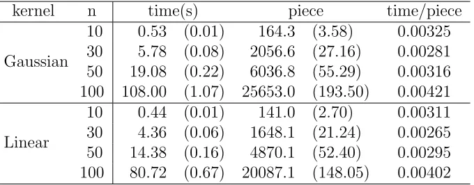
Table 2.1 Empirical computing time based on 100 independent repetitions:

the machine we used equips Intel Core (TM) i3 550 @ 3.20GHZ

CPU with 4GB memory. . . 26

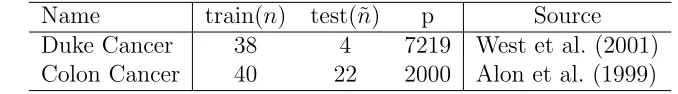
Table 2.2 Sources for the microarray data used for illustrations: The numbers

of predictors (p) are all 7219 and much larger than the sample size

(n). . . 29

Table 2.3 Test CREs for Microarray data sets (p > n). . . 29

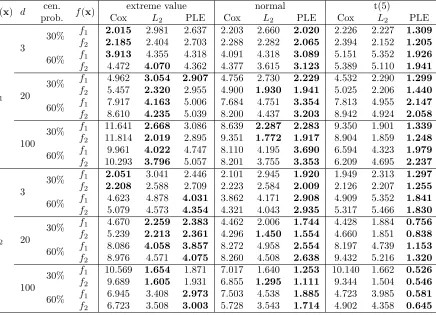
Table 3.1 The proposed PLE outperforms both standard and L2-penalized

Cox model if the PH assumption is violated. Bold case is used to

represent a winning estimator in terms of ¯DRISE in each scenario.

In some cases, two methods are marked in bold together since their diﬀerences are not statistically signiﬁcant. Quartiles of the standard

errors of all the entries are Q1 =.118, Q2 =.174, and Q3 =.368. . 44

Table 4.1 Averaged Frobenius distances betweenPBandP_Bˆ over 100

indepen-dent repetitions are shown under various scenarios. Corresponding

standard deviations are given in parentheses. . . 60

Table 4.2 The ﬁrst ﬁve leading eigenvalues (λ1,· · · , λ5) of the candidate

ma-trices estimated by diﬀerent SDR methods for the WDBC data. Cumulative ratios of the values in percentage are given in parentheses. 61

Table 4.3 Averaged test error rates (in percentage) of thek-nearest neighbor

classiﬁer (k = 3,5,7,9) over 100 random partitions for the WDBC

data with respect to the ﬁrstdsuﬃcient predictors (d = 1,2,3,4,5),

which are estimated by SDR methods. Corresponding standard

de-viations are given in parentheses. . . 64

Table 5.1 Averaged distance measures deﬁned in (5.23) over 100 independent

repetitions. The corresponding standard deviations are in parentheses 79

Table 5.2 Empirical probabilities (in percentage) of correctly estimating true

k based on 100 independent repetitions: The CVBIC procedure

for the linear WPSVM outperforms the permutation test for SAVE

estimator and shows promising result whenn = 1000. . . 80

Table 5.3 Averaged test error rates (in percentage) of theκ-NN classiﬁer (κ =

3) over 100 random partitions for the WDBC data with respect to

the ﬁrstksuﬃcient predictors (k = 1,2,3,4,5), which are estimated

by diﬀerent SDR methods. Corresponding standard deviations are

(12)

Table 5.4 Averaged test error rates (in percentage) of theκ-NN classiﬁer (κ = 3) over 100 random partitions for the WDBC data with respect to

the ﬁrstksuﬃcient predictors (k = 1,2,3,4,5), which are estimated

by diﬀerent SDR methods. Corresponding standard deviations are

(13)

LIST OF FIGURES

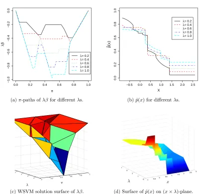
Figure 2.1 Simulated toy example: the top two panels depict the solution λβ

and the estimate ˆp(x) given by ﬁve marginalπ-solution paths, with

λ values ﬁxed at 0.2,0.4,0.6,0.8,1.0. The bottom two panels plot

the joint solution surface of λβ and the corresponding surface of

ˆ

p(x). Notice that the horizontal axis of (b) is x. Similarly the

surface in (d) lies on the (x×λ) plane. . . 11

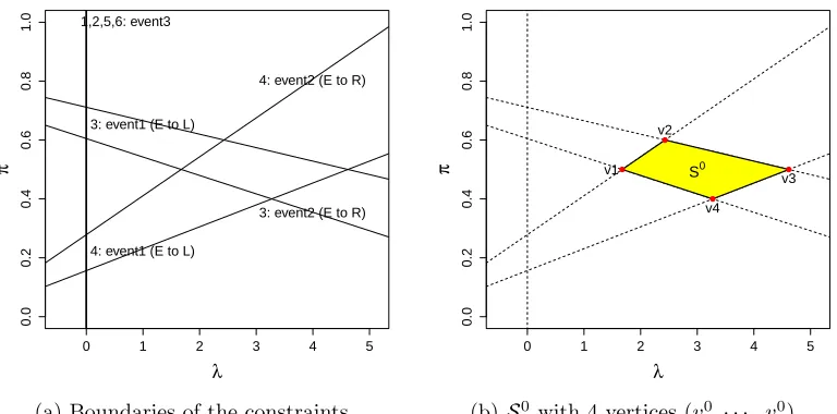
Figure 2.2 The illustration of deﬁning S0 _{generated from the initial point}

(λ0, π0) for the toy example in Section 2.1: Each line in the left

penal (a) represents a constraint boundary where an event occurs

as labeled. For example, the upper right label represents the event:

the fourth example moves from E to R on the boundary. The set

S0 _{obtained from the boundaries in (a) is depicted in (b).} _{. . . .} ₁₈

Figure 2.3 The updated polygons S1

r, r = 1,· · · ,4 from the middle points

m1,· · · , m4 of the sides of S0 in Figure 2.2 (b): Dotted lines in each subﬁgure depict the boundaries of constrains for obtaining

the polygon. . . 20

Figure 2.4 Illustration of the reﬁning step and its eﬀect for simulated example:

The left penal (a) shows all the boundaries of constraints. Dashed

(red) lines represents boundaries of constraints with b < 0 and

only two constraints (bold) are used to deﬁnedSℓ_{and the other two}

excluded are chosen by comparingπvalues atλ= 0 andλ0. Dotted

(blue) lines are the ones withb >0 and we can exclude dominated

constraints in a similar manner. The right panel (b) shows dramatic saving in computation after use of the reﬁning step by comparing

the numbers of intersection points of unreﬁned constraints (nc) and

reﬁned ones (˜nc) as functions of sample size, n. . . 24

Figure 2.5 Real data illustration onkyphosis data. . . 27

Figure 3.1 Two-dimensional solution surfaces of CKQR for the Myeloma data:

The left penal (a) shows vertices of the Sℓ_{s produced from the}

proposed algorithm and the right panel (b) depicts the solution

surface of ˆθ48. . . 41

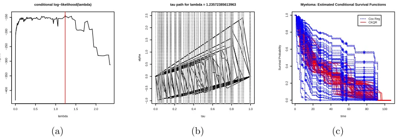
Figure 3.2 The piecewise linear conditional survival function estimator for

Myeloma Data: the left panel (a) shows cross-validated conditional

log-likelihood for diﬀerent λ and the (red) vertical line represents

the optimalλopt which maximizes the conditional log-likelihood; in

the middle panel (b), solution paths of ˆθ1,· · · ,θˆ48 as a function τ

for the λopt are depicted; the right panel (c) shows estimated CSF

(14)

Figure 3.3 The piecewise linear conditional survival function estimator for

Lymphoma Data: the proposed piecewise linear CSF estimator and

theL2-penalized Cox regression give quite diﬀerent shapes of

func-tions. . . 47

Figure 4.1 Results of classical SDR methods for WDBC data: panel (a) plots

the response versus the suﬃcient dimension reduction predictor estimated by SIR; panels (b) and (c) show the ﬁrst two directions ˆ

b⊤₁xvs. ˆb⊤₂xestimated by SAVE and pHd, respectively. Here blue

circle denotes one class while red plus the other. . . 51

Figure 4.2 Solution path of ˆf(x) for simulated example: Vertical lines

repre-sent ˆπi, i= 1,· · ·, n using the average-type deﬁnition. . . 56

Figure 4.3 Probability-enhanced SDR for WDBC data: Scatter plots of the

ﬁrst two suﬃcient predictors estimated by PRE-SIR1, PRE-SIR2,

and PRE-CUME are depicted, respectively. . . 62

Figure 5.1 π-path of the WPSVM solution ˆβ_n: The π-path algorithm

eﬃ-ciently computes complete solutions of ˆβ_n for all π ∈ [0,1] by

taking advantage of the piecewise linearity property. Ten

piece-wise linear (red) paths are shown since p= 10. The (blue) dotted

vertical lines represent pre-speciﬁed gird ofπ = (1,· · · ,9)/10. . . 70

Figure 5.2 Surface plots of the last two functionsf4 and f5: the functionf4 is

almost symmetric about the origin to a certain degree and the last

f5 is exactly symmetric about the origin. . . 78

Figure 5.3 Nonlinear SDR results for a data set from f5: The top-right panel

(a) depicts original predictors on the (X1 ×X2) plane. The rest

of three panels (b), (c), and (d) show scatter plots of the ﬁrst two suﬃcient predictors estimated by SAVE, linear WPSVM, and nonlinear WPSVM, respectively. It is clearly observed that the

kernel WPSVM performs very well while the linear WPSVM fails. 82

Figure 5.4 SDR results for WDBC data: The ﬁrst panel (a) depicts a values

ofGn(k) for allk = 1,· · · ,30 withρ=.009 chosen by ﬁve-fold CV

and shows that the selected ˆk is 3. In the panel (b), 3D-scatter plot

(since ˆk = 3) of predictors on estimated SY_|x. The last panel (c)

shows scatter plot of the ﬁrst two suﬃcient predictors estimated by

(15)

Chapter 1 Introduction

High-dimensional data are frequently encountered in a variety of applications as related

techniques for collecting, storing, and processing data advance rapidly. In this thesis

which consists of four inter-related topics, we develop new statistical tools to analyze

such high-dimensional data based on weighted learning.

1.1 Weighted Support Vector Machines

In binary classiﬁcation, we are given a set of data {(xi, yi), i= 1,· · · , n} of size n where

xi ∈ Rp and yi ∈ {−1,+1} denote a p-dimensional predictor and a binary response. Its

goal is to construct a reasonable classiﬁcation rule. Among many others, the support

vector machine (SVM) (Vapnik, 1996) is one of the most well known classiﬁers. It has

gained much popularity since its introduction. It originates with the simple idea of ﬁnding

an optimal hyperplane to separate two classes. The hyperplane is optimal in the sense

that the geometric margin between these two classes is maximized. Later it was shown by Wahba (1999) that the SVM can be ﬁt in the general regularization framework by

solving

min

f∈F n ∑

i=1

H1(yif(xi)) +

λ

2J(f), (1.1)

where H1(u) = max(1 − u,0) is the hinge loss function, J(f) denotes the roughness

penalty of a functionf(·) in a function spaceF, and the sign off(x) for a given predictor

x will be used for class prediction. Here λ > 0 is a regularization parameter which

(16)

roughness penalty. A common choice of the penalty is J(f) = ∥f∥2

F. Other choices

include the l1-norm penalty (Zhu et al., 2003; Wang and Shen, 2007) and the SCAD

penalty (Zhang et al., 2006). In general, we setF to be the Reproducing Kernel Hilbert

Space (RKHS, Wahba, 1990) HK, generated by a non-negative deﬁnite kernel K(·,·).

By the Representer Theorem (Kimeldorf and Wahba, 1971), the optimizer of (1.1) has a

ﬁnite dimensional representation given by

f(x) = b+

n ∑

i=1

θiK(x,xi). (1.2)

Due to (1.2),∥f∥2

F =

∑n i=1

∑n

j=1θiθjK(xi,xj). Then the SVM estimatesf(x) by solving

min

b,θ1,···,θn

n ∑

i=1

H1

(

yi [

b+

n ∑

j=1

θjK(xi,xj) ])

+λ

2

n ∑

i=1

n ∑

j=1

θiθjK(xi,xj). (1.3)

Note that, in the standard SVM, each observation is treated equally no matter which

class it belongs to. Yet this may not be always optimal. In some situations, it is desired

to assign different weights to the observations from different classes; one such example is when one type of misclassification induces a larger cost than the other type of

mis-classiﬁcation. Motivated by this, Lin et al. (2004) considered a broader class of learning,

the so-called weighted SVM (WSVM) by incorporating a weight parameter to adjust the

imbalance between the two classes. The WSVM solves

min

b,θ1,···,θn

n ∑

i=1

πiH1

(

yi [

b+

n ∑

j=1

θjK(xi,xj) ])

+ λ

2

n ∑

i=1

n ∑

j=1

θiθjK(xi,xj), (1.4)

where the weight πi’s are given by

πi ≡π(yi) = {

1−π if yi = +1

π if yi =−1

with π∈(0,1). Each point (xi, yi) is associated with one weight parameterπi, the value

of which depends on the label yi. Advantages of the weighted SVM include ﬂexibility

(17)

1.1.1 Probability Estimation

Besides learning a classiﬁcation boundary, one important application of the WSVM is

estimating conditional probability proposed by Wang et al. (2008), which is motivated

by the Fisher consistency of the Hinge loss shown by Lin (2002). According to Lin et al.

(2004), the WSVM classiﬁer provides a consistent estimate of sign(p(x)−π) for anyx,

where p(x) is the conditional class probability p(x) = P(Y = 1|X = x). Using this

fact, Wang et al. (2008) proposed the WSVM-based probability estimation. The basic

idea is to divide and conquer by converting a probability estimation problem into many

classification sub-problems. Each classification sub-problem is assigned with a different

weight parameter π, and these sub-problems are solved separately. Then the solutions

are assembled together to construct the ﬁnal probability estimator. A more detailed

description is as follows. Consider a sequence of 0 < π(1) _< · · · _{< π}(M) _< _{1. For each}

m = 1,· · · , M, solve the (1.4) associated with π(m) and denote the solution by ˆfm(·).

Finally, for anyx, construct the probability estimator as ˆp(x) = {π(m+)+π(m−)}/2, where

m+ = argmax_mfˆm(x) > 0 and m− = argminmfˆm(x) < 0. The proposed probability

estimator naturally enjoys the aforementioned advantages of the WSVM.

1.1.2 Solution paths of the WSVM

In a regularization framework, it is very common to study the regularization path of the

SVM solution in order to automate the selection procedure of the regularization

param-eter λ. Hastie et al. (2004) showed that the SVM solutions move in a piecewise linear

manner as a function ofλand proposed an eﬃcient solution path algorithm. Its extension

to the WSVM is straightforward since the piecewise linearity of the regularization paths

comes from the combination of anL1-type loss and anL2-type penalty in (1.3) and

incor-porating a weight parameter does not break the particular structure down. We refer to

the regularization path as λ-paths in order to emphasize the solution paths as a function

of λ. On the other hand, the WSVM solutions can be regarded as a function ofπ for a

given λ and we can deﬁne π-paths analogous to the λ-paths. The piecewise linearity of

the π-path was established by Wang et al. (2008). Complete π-paths of the WSVM can

facilitate the implementation of the probability estimation procedure. However, unlike

marginal solution paths, it is largely unknown how the WSVM solutions move as the two

(18)

1.1.3 Connection to Kernel Quantile Regressions

The quantile regression is a very popular as an alternative of the mean regression and is

characterized by the check loss ρτ(u) deﬁned by

ρτ(u) = {

τ u, if u≥0

−(1−τ)u, if u <0,

where τ ∈ [0,1] is referred to as a quantile parameter since it controls a target quantile

of interest. The kernel quantile regression (KQR, Takeuchi et al., 2006; Li et al., 2007)

solves the following optimization problem deﬁned on the RKHS.

min

f∈HK

n ∑

i=1

ρτ(yi−f(xi)) +

λ

2∥f∥ 2

HK.

The only diﬀerence of the KQR from the SVM is that the hinge loss is replaced with

the check loss. Moreover these loss functions are very closely related as shown in the

following. For any a∈[−1,1] andy={−1,1}, the check loss with a quantile parameter

τ given is

ρτ(y−a) =ρτ(y(1−ya)) = {

τ|1−ya|, if y = 1

−(1−τ)|1−ya|, if y =−1.

That is, the KQR is theoretically equivalent to the WSVM if the response is binary.

1.2 Suﬃcient Dimension Reduction

High dimensional data become more popular as related data acquisition and storage techniques advance. In modern statistics, it is not optional but essential to reduce

di-mensionality of the data without loss of information.

In this context, suﬃcient dimension reduction (SDR) has been developed under less

stringent model assumption as follows. SDR assumes

(19)

notes statistical independence, and B is a p×k-dimensional matrix. In other words,

the dependent structure between Y and X is only through B⊤X. The model (1.5) is

very ﬂexible and covers a lot of statistical models since it does not assume any speciﬁc

relation betweenX andY but the conditional independence. Under model (1.5), SDR is

achieved by estimating B and hence the matrix B or more precisely the space spanned

by it, which is referred to as dimension-reduction subspace, is a target of interest in the

SDR. However, B itself is not identiﬁable since any full-rank linear combination of B

satisﬁes (1.5) as long as B does. The central subspace denoted by SY_|x is deﬁned as the

intersection of all dimension-reduction subspaces satisfying (1.5). SY_|x has the lowest

di-mension among all didi-mension-reduction subspaces. Under mild conditions,SY_|x uniquely

exists (Cook, 1996, 1998b). We assume the unique existence ofSY_|x andSY|x= span(B)

throughout this article. The dimension of B, k is called structure dimensionality in the

literature and its estimation is another important step in SDR.

One often refers to (1.5) as linear SDR. As a nonlinear generalization of linear SDR,

Cook (2007) introduce nonlinear SDR which assumes

Y ⊥X|ϕ(X), (1.6)

whereϕ:Rp _7→_Rk _{is an arbitrary function of}_X_{. Under model (1.6), SDR is achieved by}

obtaining a functionϕ which need not to be linear. Similar to linear SDR, the unknown

function ϕ is not unique, but is assumed to be unique modulo injective transformation

to guarantee its identiﬁability.

1.2.1 Existing SDR methods

There are a variety of methods developed for suﬃcient dimension reduction in the

liter-ature. Toward linear SDR, sliced inverse regression (SIR; Li, 1991) is the most popular

method in the literature. Many linear SDR methods have been developed since SIR was

introduced and these include, but are not limited to, sliced averaged variance estimator (SAVE, Cook and Weisberg, 1991), principal Hessian direction (pHd, Li, 1992; Cook,

1998a), iterative Hessian transformation (IHT, Cook and Li, 2002), Fourier method (Zhu

and Zeng, 2006), and directional regression (DR, Li and Wang, 2007). For nonlinear

SDR, several methods have been recently proposed by extending idea of SIR. See for

(20)

1.2.2 Diﬃculties in Binary Classiﬁcation

SDR originally arises in the regression context. The performance of most SDR methods

may suﬀer severely when the response is binary. For example, SIR can estimate at

most one direction of SY_|x and SAVE is known for its ineﬃciency when the response is

binary (Li and Wang, 2007). This is not surprising since both methods slice predictors

according to the order of response to estimate inverse regression curve and hence become ineﬀective with a binary response. Cook (1998b) discussed the diﬃculty of SDR for

binary classiﬁcation in its whole Chapter 5.

Binary classiﬁcation with high-dimensional data is commonly encountered in a variety

of applications such as clinical trials, genetics, ﬁnance, engineering, and computer science.

Thus, it is desired to develop an eﬃcient method to reduce dimension of the data without

loss of information with binary response.

1.3 Outline of the Thesis

The ﬁrst two chapters are about two dimensional solution surfaces of the WSVM and

the (weighted) KQR, respectively. In Chapter two, we ﬁrst establish that the WSVM

solutions are jointly piecewise linear with respect to the regularization and the weight

parameter, which enables us to develop a state-of-the-art algorithm that can compute the

entire trajectory of the WSVM solutions for every parameter pair at a feasible

computa-tional cost. The derived two-dimensional solution surface provides theoretical insight on

the behavior of the WSVM solutions. Numerically, the algorithm can greatly facilitate

the implementation of the WSVM and automate the selection process of the optimal reg-ularization parameter. In Chapter three, motivated by the closed connection between the

WSVM and the KQR, we propose a piecewise linear conditional survival function (CSF)

estimator from the two dimensional solution surfaces of the censored kernel quantile

re-gression (CKQR) that we developed for censored survival data. The solution surfaces

contain complete information of the CKQR for any arbitrary pairs of the regularization

and the quantile parameter, which naturally leads a CSF estimator by aggregating the

information from the complete solution surfaces. The proposed CSF estimator which is

(21)

Chapter four, probability-enhanced SDR scheme is proposed. Its key idea is to slice

data based on the conditional class probability p(x) rather than the binary response y.

We ﬁrst show that the central subspace based on p(x) is the same as that based on y.

This important result justiﬁes the proposed slicing scheme from a theoretical perspective

and assures no information loss. In practice, the true conditional class probability is

generally not available, and probability estimation can be challenging for data with

large-dimensional inputs. We further show that, to implement the new slicing scheme, one does

not need exact probability values, and all the required information is the relative order of

the probability values. Motivated by this, our new SDR procedure bypasses probability

estimation, and employs Fisher consistency of the WSVM to directly estimates the order of probability values, based on which the slicing is done. In Chapter ﬁve, we introduce

weighted principal support vector machine (WPSVM) for SDR in binary classiﬁcation

by extending the idea of principal support vector machine recently developed by Li et al.

(2011) in the context of regression. The proposed WPSVM preserves all the merits of

PSVM and successfully achieves SDR in binary classiﬁcation. Its estimation become very

(22)

Chapter 2 Two-Dimensional Solution Surface

for Weighted Support Vector

Machines

2.1 Introduction

Frequently encountered in real applications is binary classiﬁcation, in which we are given

a training set {(xi, yi), i = 1,· · · , n} of size n and the goal is to learn a classiﬁcation

rule. Here xi ∈ Rp and yi ∈ {−1,1} denote a p-dimensional predictor and a binary

response (or class label), respectively, for the ith example. The primary goal of the

binary classiﬁcation is to construct a classiﬁer which can be used for class prediction

of new objects with predictors given. The (weighted) SVM is one of the most popular

classiﬁcation methods in this context.

Besides learning the classiﬁcation boundary, one of their important applications is

to estimate class probabilities introduced in Section 1.1.1. One main concern about the

probability estimation scheme is its computational cost. The cost comes from two sources:

there are multiple sub-problems to solve, since the weight parameter π varies in (0,1);

each sub-problem is associated with one regularization parameter λ, which needs to be

adaptively tuned in the range (0,∞). To facilitate the computation, theλ-path algorithm

(23)

unknown how the WSVM solution changes when both the regularization parameterλand

the weight parameterπvary together. The main purpose of our two-dimensional solution

surface is to reduce the computation and tuning burden by automatically obtaining the

solutions for all possible (π, λ) with an eﬃcient algorithm.

One main motivation of this paper is to study the behaviors of the entire WSVM

so-lutions and characterize them by a simple representation form through their relationship

toπand λ. We use subscripts to emphasize that the WSVM solutionf is a function ofλ

andπ and sometimes omit the subscripts when they are clear from the context. Another

motivation for the need of the solution surface is to automate the selection of the

reg-ularization parameter and improve the eﬃciency of searching process. Although Wang et al. (2008)’s conditional class probability estimator performs well as demonstrated by

their numerical examples, its performance depends heavily on λ. They proposed to tune

λby using a grid search in their numerical illustrations. Yet, it is well known that such a

grid search can be computationally ineﬃcient and, in addition, its performance depends

on how ﬁne the grid is. The above discussions motivate us to develop a two-dimensional

solution surface (rather than a one-dimensional path) as a continuous function of both λ

andπ in the analogous way that one resolved the ineﬃciency of the grid search for

select-ing the regularization parameter λof the SVM by computing the entire λ-regularization

path (Hastie et al., 2004). From now on, we refer to the new two-dimensional solution

surface of the WSVM as the WSVM solution surface.

In order to show the diﬃculties in tuning the regularization parameter for the

prob-ability estimation (Wang et al., 2008) and motivate our new tuning method based on

the WSVM solution surface, we use a univariate toy example generated from a Gaussian

mixture: xi is randomly drawn from the standard normal distribution ifyi = 1 and from

N(1,1) otherwise, with ﬁve points from each class. The linear kernel (K(xi, xj) =xixj)

is employed for the WSVM and its solution is then given by f(x) = b + βx with

β = ∑n_i₌₁θixi. In order to describe the behavior of f(x), we plot λβ based on the

obtained WSVM solution surface (or path), since λβ, instead of β, is piecewise-linear in

λdue to our parametrization. In Figure 2.1, the top two panels depict the solution paths

of λβ for the diﬀerent values of λ ﬁxed at 0.2,0.4,0.6,0.8,1.0 (left) and the

correspond-ing estimates of ˆp(·) as a function of x (right); the bottom two panels plot the entire

two-dimensional joint solution surface (left) and the corresponding probability estimate

ˆ

(24)

are piecewise-linear in π they have quite diﬀerent shapes for diﬀerent values of λ (see

(a)). Thus the corresponding probability estimates can be quite diﬀerent even for the

same x(see (b)), suggesting the importance of selecting an optimal λ. By using the

pro-posed WSVM solution surface, we can completely recover the WSVM solutions on the

whole (λ×π)-plane (see (c)), which enables us to produce the corresponding conditional

probability estimators at a given x for every λ with very little computational expense

(see (d)). We will shortly demonstrate that it is computationally eﬃcient to extract

marginal paths (λ-path or π-path) once the WSVM solution surface is obtained. In this

example, we use a grid of ﬁve equally-spaced λs which is very rough. In practice, it is

typically not known a priori how ﬁne the grid should be or what the appropriate range

of the grid is. If the data are very large or complicated, the grid one choose may not be

ﬁne enough to capture the variation of the WSVM solution and will lose eﬃciency for

the subsequent probability estimation. The proposed WSVM solution surface provides

a complete portrait for the WSVM solution corresponding to any pair of λ and π and

therefore naturally overcomes this kind of practical diﬃculties, in addition to the gain in

computational eﬃciency.

In this article, we show that the WSVM solution is jointly piecewise-linear in both

λ and π and propose an eﬃcient algorithm to construct the entire solution surface on

the (λ×π)-plane by taking advantage of the established joint piecewise-linearity. As a

straightforward application, an adaptive grid for tuning the regularization parameter of

the probability estimation scheme (Wang et al., 2008) is proposed. We ﬁnally remark

that the WSVM solution surface has broad applications in addition to the probability

estimation.

2.2 Problem Setup

By introducing nonnegative slack variables ξi, i = 1,· · · , n and using inequality

con-straints, the WSVM problem (1.4) can be equivalently rewritten as

min

b,θ1,···,θn

n ∑

i=1

πiξi+

λ

2

n ∑

i=1

n ∑

j=1

θiθjK(xi,xj)

(25)

0.0 0.2 0.4 0.6 0.8 1.0

−1.0

−0.8

−0.6

−0.4

−0.2

0.0

π

λβ

λ= 0.2

λ= 0.4

λ= 0.6

λ= 0.8

λ= 1.0

(a)π-paths ofλβ for diﬀerentλs.

−0.5 0.0 0.5 1.0 1.5 2.0 2.5

0.0

0.2

0.4

0.6

0.8

1.0

X

p^

(

x

)

λ= 0.2

λ= 0.4

λ= 0.6

λ= 0.8

λ= 1.0

(b) ˆp(x) for diﬀerentλs.

1 2

3 4

0 0.2

0.4 0.6

0.8 1

π λ

(c) WSVM solution surface ofλβ. (d) Surface of ˆp(x) on (x×λ)-plane.

Figure 2.1: Simulated toy example: the top two panels depict the solution λβ and

the estimate ˆp(x) given by ﬁve marginal π-solution paths, with λ values ﬁxed at

0.2,0.4,0.6,0.8,1.0. The bottom two panels plot the joint solution surface of λβ and

the corresponding surface of ˆp(x). Notice that the horizontal axis of (b) is x. Similarly

(26)

The corresponding Lagrangian primal function is constructed as

LP : n ∑

i=1

πiξi+

λ

2

n ∑

i=1

n ∑

j=1

θiθjK(xi,xj) + n ∑

i=1

αi(1−yif(xi))− n ∑

i=1

γiξi, (2.1)

where αi ≥0 andγi ≥0 are the Lagrange multipliers. To derive the corresponding dual

problem, we set the partial derivatives ofLP in (2.1) with respect to the primal variables

to zero, which gives

∂ ∂θi

:

n ∑

j=1

θjK(xi,xj) =

1

λ

n ∑

j=1

αjyjK(xi,xj), (2.2)

∂ ∂b :

n ∑

i=1

αiyi = 0, (2.3)

∂ ∂ξi

: αi =πi−γi, (2.4)

along with the Krush-Kuhn-Turker (KKT) conditions

αi[1−yif(xi)−ξi] = 0, (2.5)

γiξi = 0. (2.6)

Notice from (2.2) that the function (1.2) can be rewritten as

f(x) = b+ 1

λ

n ∑

i=1

αiyiK(x,xi). (2.7)

By combining (2.2-2.6), the dual problem of the WSVM is given by

max

α1,···,αn

n ∑

i=1

αi −

1 2λ

n ∑

i=1

n ∑

j=1

αiαjyiyjK(xi,xj) (2.8)

subject to

n ∑

i=1

yiαi = 0 and 0 ≤αi ≤πi, ∀i= 1,· · · , n.

(27)

to select the desired λ and π. This is very computationally intensive for large data set

because the QP itself is a numerical method whose computational complexity increases

polynomially in n.

For the standard SVM (equivalent to a special case of the WSVM with the weight

parameter π = 0.5), Hastie et al. (2004) showed the piecewise-linearity of αi in λ and

developed an eﬃcient algorithm to compute the entire piecewise-linear solution path.

The same idea can be extended straightforwardly to the WSVM with any ﬁxed weight

parameter or any ﬁxed individual weights. In addition, Wang et al. (2008) showed the

WSVM solutions αi are piecewise-linear in the weight parameter π while keeping the

regularization parameterλﬁxed. However it is largely unknown how the WSVM solution

αi changes with respect to the two parameters jointly. In this article, we show that the

WSVM solutions αis, as a function of both λ and π, form a continuous piecewise-linear

solution surface on the (λ×π)-plane and propose an eﬃcient algorithm to compute the

entire solution surface.

Similar to the idea of Hastie et al. (2004), we categorize all the examples, i= 1,· · · , n

into the three disjoint sets as

E ={i:yif(xi) = 1, 0≤αi ≤πi} (elbow),

L={i:yif(xi)<1, αi =πi} (left),

R={i:yif(xi)>1, αi = 0} (right).

It is easy to see that the above three sets are always deﬁned uniquely by the conditions

(2.2)-(2.6). The set names come from the particular shape of the hinge loss function

(Hastie et al., 2004). Note that{αi,∀i∈ E}contains most of the information on how the

WSVM solution changes on the (λ×π)-plane, since the rest solutions {αi, i ∈ L ∪ R}

are trivially determined by the deﬁnition of the sets.

As λ and π change, the sets may change and, as long as this happens, we call it an

event. All the solution surfaces forαi, i= 1,· · · , n are continuous and hence no element

inL can move directly toRor vice versa. Therefore there are only three possible events

to be considered as follows. The ﬁrst event deﬁnes when one of αi, i ∈ E reaches πi

and the corresponding index i exits from E to L (event 1). Similarly, an αi, i ∈ E can

reach the other boundary 0 and the index moves form E toR (event 2). The last event

(28)

2.3 Joint piecewise-linearity

In this section, we study the behavior of the WSVM solutions from a theoretical point of

view. One major discovery we have made is that,αi, i∈ E, hence all the αi, i= 1,· · · , n

changes in a jointly piecewise-linear manner when λ and π vary. The following theorem

describes howαi moves asλ and π change. For simplicity, we deﬁneα0 =λb.

Theorem 1. (Joint Piecewise-Linearity) Suppose we have a point (λℓ, πℓ) in the (λ× π) plane. Let Eℓ, Lℓ, Rℓ, αℓ = (αℓ₁,· · ·, α_nℓ)T, and αℓ₀ denote the associated sets and solutions obtained at (λℓ_{, π}ℓ_{), respectively. Now, we consider a subset} _Sℓ _{(of the} ₍_λ_×_π₎ -plane) which contains (λℓ_{, π}ℓ₎ _{such that no event happens within} _Sℓ_{. In other words, for} all (λ, π) ∈ Sℓ_{, the associated three sets,} _E_, _L_{, and} _R _{remain the same as} _Eℓ_, _Lℓ_{, and} Rℓ_{, respectively. Then the solution} _α

i, i ∈ {0} ∪ Eℓ, denoted by α0,E in a vector form moves in Sℓ _{as follows:}

α0,E ≡α0,E(λ, π) = αℓ0,E +Gℓ∆, ∀ (λ, π)∈ Sℓ, (2.9)

where αℓ

0,E ={αℓi :i∈ {0} ∪ Eℓ} and ∆= (∆λ,∆π)T = (λ−λℓ, π−πℓ)T. The gradient matrix, Gℓ is given by

Gℓ =A−ℓ1Bℓ= (

0 yT

ℓ yℓ K∗ℓ

)−1(

0 |Lℓ_|

1 −k∗_ℓ )

, (2.10)

where K∗_ℓ = {yiyjK(xi,xj) : for i, j ∈ Eℓ}; k∗ℓ = { ∑

j∈LℓyiK(xi,xj) : i ∈ Eℓ}T; yℓ = {yi : i ∈ Eℓ}T; |A| denotes the cardinality of a set A; and 1 is the one vector of length |Eℓ_|_.

The proof of Theorem 1 is given in Appendix A.1. We remark that Aℓ is rarely

singular in practice, and related discussions can be found in Hastie et al. (2004). It is

worthwhile to point out that the joint piecewise-linearity of the solution guarantees the

marginal piecewise-linearity as presented in Corollary 2, but not vice versa. Therefore,

Theorem 1 implies the piecewise-linearity of the marginal solution paths as a function

(29)

linearly in λ∈ {λ: (λ, π0)∈ Sℓ} as follows.

α0,E =αℓ0,E+g ℓ

1∆λ.

Similarly, α0,E changes in π∈ {π : (λ0, π)∈ Sℓ} for a given λ0 as follows.

α0,E =αℓ0,E +g ℓ

2∆π, where gℓ

1 and gℓ2 denote the first and second column vectors ofGℓ in (2.10), respectively.

The classiﬁcation function f(x) can be conveniently updated by plugging (2.9) into

(A.1), which gives

f(x) = λ

ℓ

λ

[

fℓ(x)−hℓ₁(x)]+hℓ₁(x) + π−π

ℓ

λ h

ℓ

2(x), (2.11)

where

hℓ₁(x) = g01+

∑

i∈Eℓ

gi1yiK(x,xi),

hℓ₂(x) = g02+

∑

i∈Eℓ

gi2yiK(x,xi) + ∑

i∈Lℓ

K(x,xi),

and (gi1, gi2) denotes the row ofGℓ wherei∈ {0} ∪Eℓ. We observe from (2.11) thatf(x)

is not jointly piecewise-linear in (λ, π) while it is marginally piecewise-linear inλ−1 and

π, respectively.

2.4 Solution Surface Algorithm

In this section, we propose an eﬃcient algorithm to compute the entire solution surface

of the WSVM on the (λ×π)-plane by using the joint piecewise-linearity established in

Theorem 1.

2.4.1 Initialization

Denote index sets I+ ={i :yi = 1} and I− ={i:yi =−1}. We initialize the algorithm

(30)

∑

i∈I+πi(π0) = ∑

i∈I−πi(π0). Withπ=π0 it is easy to verify that, for a suﬃciently large

λ, αi =π0 if i∈I+ and 1−π0 otherwise. Following the idea of Hastie et al. (2004), the

initial values of λ and α0 denoted by λ0 and α00, respectively are given by

λ0 = 1 2



(1−π0)

∑

i∈I+

(K_i+−K_i−) +π0

∑

i∈I₋

(K_i+−K_i−)

  and

α0₀ =−1 2



(1−π0)

∑

i∈I+

(K_i+−K_i−)−π0

∑

i∈I−

(K_i+−K_i−)

 ,

where K_i+ =K(xi,xi+),Ki− =K(xi,xi−). The indices i+ and i− are deﬁned as

i+ = argmax

i∈I+

{(1−π0)

∑

j∈I+

K(xi,xj)−π0

∑

j∈I₋

K(xi,xj)} and

i₋ = argmin

i∈I₋ {

(1−π0)

∑

j∈I+

K(xi,xj)−π0

∑

j∈I−

K(xi,xj)}.

It is possible to initialize the algorithm at anyπbetween 0 and 1 rather thanπ0, however,

we empirically observe that the initializedλ is the largest when π=π0. Notice that the

corresponding solution is trivial as αi =πi for all i= 1,· · · , n for any λ larger than λ0.

Therefore, the proposed algorithm focuses only on the non-trivial solutions obtained at

Q = {(λ, π) : 0 ≤ λ ≤ λ0,0 ≤ π ≤ 1}. Finally, the three sets initialized at (λ0, π0)

denoted by E0,L0 and R0, respectively are given by

E0 ₌_{_i

+, i−}, L0 ={1,· · · , n}\E0, and R0 =ϕ,

where ϕ denotes the empty set.

2.4.2 Update

Recall that, for any point (λℓ_{, π}ℓ_{), no event occurs if (}_{λ, π}₎_{∈ S}ℓ _{and the WSVM solution}

can be updated by applying Theorem 1 for any (λ, π)∈ Sℓ_{. Therefore, it is essential to}

know how to deﬁne Sℓ _{as large as possible for any (}_λℓ_{, π}ℓ_{). We shall demonstrate next}

(31)

have the following inequality constraints to prevent event 1 from happening:

gi1λ+ (gi2+ 1)π ≤tℓi + 1, i∈ E ℓ

+ (2.12)

gi1λ+ (gi2−1)π ≤tℓi, i∈ E

ℓ

−, (2.13)

where tℓ

i =gi1λℓ+gi2πℓ−αℓi, E+ℓ =Eℓ∩I+ and E₋ℓ =Eℓ∩I−. In a similar way, we have

the following inequalities to prevent event 2:

gi1λ+gi2π≥tℓi, i∈ E

ℓ_. _(2.14)

In order to prevent event 3, we have yif(xi) < 1,∀i ∈ Lℓ and yif(xi) > 1,∀i ∈ Rℓ.

Therefore, by noting (A.1), we have

(hℓ₁(xi)−1)λ+h2ℓ(xi)yiπ ≤sℓi, i∈ R

ℓ _(2.15)

(hℓ₁(xi)−1)λ+h2ℓ(xi)yiπ ≥sℓi, i∈ L

ℓ

, (2.16)

where sℓ

i = yi(hℓ1(xi) −fℓ(xi))λℓ +hℓ2(xi)yiπℓ. We remark that the equalities do not

need to be strict since an eventis instant transition. Recall that it is enough to consider

the solution on Q and hence the additional constraints 0 ≤ λ ≤ λ0 and 0 ≤ π ≤ 1

should be considered as well by default. In summary Sℓ can be deﬁned by a subregion

on the (λ×π)-plane that satisﬁes all the constraints (2.12)–(2.16). Figure 2.2 illustrates

a Sℓ _{generated from the initial point (}_λ

0, π0) for the toy example in Section 2.1. We

remark that Sℓ _{forms a} _polygon _{which can be uniquely expressed by its vertices, since}

the constraints are all linear.

We describe next how to determine the vertices of Sℓ _{in an eﬃcient manner. First,}

compute all the pairwise intersection points of the boundaries of (2.12)–(2.16) then we

have nc(nc−1)

2 intersection points, where nc denotes the number of constraints (2.12)–

(2.16),n+|Eℓ|. The left penal of Figure 2.2 shows all the intersections of the boundaries of

the obtained constraints. Then, we can deﬁne the vertices by identifying the intersections that satisfy all the constraints (2.12)–(2.16) as illustrated in (b) of Figure 2.2. We denote

the vertices of the Sℓ _as _{_vℓ

1,· · · , vnℓv} where v

ℓ

r = (λr, πr), r= 1,· · · , nv.

There are a couple of issues we need to clarify here. First, based on our limited

experience, we observe that nv is small and typically does not exceed eight. Hence it is

not eﬃcient to compute all the nc(nc−1)

(32)

0 1 2 3 4 5

0.0

0.2

0.4

0.6

0.8

1.0

λ

π

3: event2 (E to R) 4: event2 (E to R)

3: event1 (E to L)

4: event1 (E to L) 1,2,5,6: event3

(a) Boundaries of the constraints.

0 1 2 3 4 5

0.0

0.2

0.4

0.6

0.8

1.0

λ

π v1 S0

v2

v3

v4

(b)S0 _{with 4 vertices (}_v0

1,· · ·, v04).

Figure 2.2: The illustration of deﬁning S0 _{generated from the initial point (}_λ

0, π0) for the toy example in Section 2.1: Each line in the left penal (a) represents a constraint

boundary where anevent occurs as labeled. For example, the upper right label represents

the event: the fourth example moves fromE toR on the boundary. The setS0 _obtained

(33)

intensity. Note also that some constraints are dominated by others onQand are thus au-tomatically satisﬁed if other constraints hold. Consequently, we can save a huge amount

of computational time by excluding those constraints which are dominated by others,

especially when n is large. We also need to order the vertices for set-updates which are

discussed next. Here the ordering means that a vertex vℓ

r, r = 1,· · · , nv is adjacent to

vℓ

r−1 and vrℓ+1, where we setv0ℓ =vnℓv, v

ℓ

nv+1 =v

ℓ

1 (see (b) in Figure 2.2). The updating of

α1,· · · , αn as well as α0 at vertices of Sℓ provided is straightforward by Theorem 1.

Figure 2.3 illustrates how to extend the polygons on Q from current Sℓ in Figure

2.2-(b). Notice that the sides ofSℓare determined by some boundaries of the constraints

(2.12) – (2.16) and represent corresponding events. Each middle point of two adjacent

vertices can be used as a new starting point, (λℓ+1_{, π}ℓ+1_{) in} _{Theorem 1} _{to compute}

a new polygon Sℓ+1_{. Computing middle points and corresponding solutions denoted}

by mr = (λℓr+1, πrℓ+1) and ¯αℓr+1 = {(α0, α1,· · · , αn) obtained at mr = (λrℓ+1, πℓr+1)}T,

respectively where r = 1,· · · , nv is trivial due to the piecewise-linearity of the solutions.

The bar sign in ¯αℓ+1

r is used to emphasize the quantities are obtained at middle points,

not vertices. At each middle point, the corresponding three sets denoted by E_rℓ+1,Rℓ_r+1,

and Lℓ_r+1 respectively can be updated based on which line the middle point mr is on.

For example as shown in (a) of Figure 2.3, the three sets E₁ℓ+1,R₁ℓ+1, and Lℓ₁+1 obtained

at m1 are updated as E1ℓ+1 =Eℓ\{4},R

ℓ+1

1 =Rℓ∪ {4}, and L

ℓ+1

1 =Lℓ. This is because

m1 = (λℓ1+1, π

ℓ+1

1 ) lies on the boundary which represents an event that the element 4

moves to the right set from the elbow set (see (a) in Figure 2.2). Now we have all the

information required to generate a new polygon, S₁ℓ+1, from the middle point, m1 and

Sℓ+1

1 can be accordingly computed by treating m1 as a new updating point (This is

the reason why we use a superscript ℓ + 1 to denote middle points). Figure 2.3 shows

all the four newly-created polygons, S1

r, r = 1,· · · ,4 respectively from the four middle

points m1,· · · , m4 of the sides of S0 in Figure 2.2-(b). Notice that the right vertical

line represents λ=λ0 and we do not have any interest beyond it. Finally, the proposed

algorithm can be continued to extend the polygons being searched onQand is terminated

when the complete solution surface is recovered onQ.

2.4.3 Resolving Empty Elbow

Note that either event 1 and or event 2 leads to the possibility that E is empty, named

(34)

0 1 2 3 4

0.0

0.2

0.4

0.6

0.8

1.0

Updated polygon from m1

λ

π S₁1

m1

(a)S1

1 fromm1.

0 1 2 3 4

0.0

0.2

0.4

0.6

0.8

1.0

λ

π m2 S₂1

(b)S1

2 fromm2.

0 1 2 3 4

0.0

0.2

0.4

0.6

0.8

1.0

λ

π S₃1 m3

(c)S1

3 fromm3.

0 1 2 3 4

0.0

0.2

0.4

0.6

0.8

1.0

λ

π S₄1

m4

(d)S1

4 fromm4.

Figure 2.3: The updated polygons S1

r, r = 1,· · · ,4 from the middle pointsm1,· · · , m4

of the sides ofS0 _{in Figure 2.2 (b): Dotted lines in each subﬁgure depict the boundaries}

(35)

Theorem 1 cannot be applied whenE is empty.

We suppose theempty elbow occurs at (λo_{, π}o_{) and use a superscript ‘}_o_{’ to denote any}

quantity deﬁned at (λo_{, π}o_{). In order to resolve the} _{empty elbow}_{, we ﬁrst notice that the}

objective function (1.4) is diﬀerentiable with respect to b and αi, i= 1,· · · , n whenever

the the elbow set is empty since in this case there is no example satisfying yif(xi) = 1.

Taking derivative of (1.4) with respect to b and αi, we get two conditions to be satisﬁed

under the empty elbow: i) πo = |Lo₊|/|Lo|, where Lo₊ = Lo∩I+ and ii) αi are unique

while α0 is not. Moreover, α0 can be any value in the following interval,

[aL, aU], [

max

i∈Lo −∪Ro+

mo_i, min

i∈Lo

+∪Ro−

mo_i

]

(2.17)

where mo_i = yiλo−

∑n j=1α

o

jyjK(xi,xj); and Lo₋, Ro+, and Ro− are similarly deﬁned as

Lo

+. Recall that α0 is continuous and hence the empty elbow can be resolved only by

α0 touching one of the two boundaries aL and aU. Notice that the α0o is regarded as

a starting point where the empty elbow begins and hence it must be one of aL and

aU. Without loss of generality, we suppose αo0 = aL then the empty elbow should be

resolved when it becomes the other boundary aU. Let ioL = argmaxi∈Lo

−∪Ro+m o i and

io

U = argmini∈Lo

+∪Ro−m

o

i, then the E should be updated to {ioU}. The L and R are

accordingly updated as well since the updated index io_U enters to the E from one of the

two sets. In case ofαo₀ =aU, we update in a similar way which leads to E ={ioL}.

2.4.4 Pseudo Algorithm

Combining the previous several subsections, we now summarize our WSVM solution

surface algorithm at Algorithm 1. We denote α = (α0, α1,· · · , αn)T for simplicity. We

note that the proposed algorithm computes the complete WSVM solution αs for any

(λ, π) ∈ Q without involving any numerical optimization. We have implemented the

algorithm in R language and the wsvmsurf package is available from the authors upon

request (and will be available on CRAN soon).

2.5 Computational Complexity

The essential part of the proposed algorithm involves several steps. First, we solve the

New Techniques for High-Dimensional and Complex Data Analysis Based on Weighted Learning.

ABSTRACT

DEDICATION

BIOGRAPHY

ACKNOWLEDGEMENTS

TABLE OF CONTENTS

LIST OF TABLES

LIST OF FIGURES

Chapter 1

Introduction

1.1

Weighted Support Vector Machines

1.1.1

Probability Estimation

1.1.2

Solution paths of the WSVM

1.1.3

Connection to Kernel Quantile Regressions

1.2

Suﬃcient Dimension Reduction

1.2.1

Existing SDR methods

1.2.2

Diﬃculties in Binary Classiﬁcation

1.3

Outline of the Thesis

Chapter 2

Two-Dimensional Solution Surface

for Weighted Support Vector

Machines

2.1

Introduction

2.2

Problem Setup

2.3

Joint piecewise-linearity

2.4

Solution Surface Algorithm

2.4.1

Initialization

2.4.2

Update

2.4.3

Resolving Empty Elbow

2.4.4

Pseudo Algorithm

2.5

Computational Complexity