Models and Estimation Methods for Distribution of Scores for Functional Data.

(1)

ABSTRACT

TONG, ZHENTAO. Models and Estimation Methods for Distribution of Scores for Functional Data. (Under the direction of Sujit K. Ghosh).

Normal distribution is the most widely applied distribution in statistics. For example, in mixed effect modelling, those realized but latent random effects are often assumed to be normally distributed. Analagously, in functional principal component analysis, latent scores are almost always assumed to be normally distributed. Such assumption, however, may be problematic in some circumstances. In Chapter 2, we develop a non-parametric density estimation method that can be potentially applied to functional principal component analysis. We also incorporate certain moment constraints based on theories developed in functional data area.

In functional principal component analysis, typically people are interested in estimation of mean function and covariance function, as well as individual trajectory reconstruction. In contrast, probabilistic inference at a certain time point does not receive much attention in existing literature. This is because under the usual assumption of normality for functional principal component scores, probabilistic inference is trivial. However, sometimes assuming normally distributed scores might not be the best approach. In Chapter 3, we develop such probabilistic inference for the case when scores are not normally distributed. We utilize the moment constraint density estimator from Chapter 2 along with the well known Karhunen-Loeve theorem. We show through simulation studies that our method beats the Normal distribution based inference method in different scenarios.

(2)

(3)

Models and Estimation Methods for Distribution of Scores for Functional Data

by Zhentao Tong

A dissertation submitted to the Graduate Faculty of North Carolina State University

in partial fulfillment of the requirements for the Degree of

Doctor of Philosophy

Statistics

Raleigh, North Carolina

2019

APPROVED BY:

Luo Xiao Ana-Maria Staicu

Brian Reich Sujit K. Ghosh

(4)

DEDICATION

(5)

BIOGRAPHY

(6)

ACKNOWLEDGEMENTS

I would like express my sincerest gratitude to my research advisor Dr. Sujit Ghosh. Throughout my research at NC State, I am deeply impacted by his rigorous thinking, persuasive arguments and broad knowledge. His great patience and continuous support build the power that drives me forward.

I would also like to thank Dr. Ana-Maria Staicu, Dr. Brian Reich, Dr. Luo Xiao and Dr. Min Kang for serving in my doctoral committee and providing valuable advices.

I would also like to thank Dr. Howard Bondell, Dr. Donald Martin and Dr. Wenbin Lu for serving as the director of graduate program in our department. I also appreciate all other faculties and staffs who supported me through my education here.

I am also truly grateful for all my internship supervisors: Mr. Mohammed Chaara from Lenovo, Dr. Kyounghwa Bae from Janssen and Dr. Juan Li from Lilly. They helped me connecting the knowledge learned from class to those practical challenges that waits to be solved. They also demonstrated to me how to develop a promising career path in their fields.

(7)

LIST OF TABLES

Table 2.1 Specific Densities for Beta-Beta Mixture . . . 19

Table 2.2 Specific Densities for Beta-non-Beta Mixture . . . 19

Table 2.3 Dependence measure for Beta-Beta mixture . . . 20

Table 2.4 L1 for Beta mixture case . . . 23

Table 2.5 Moment Bias for Beta case . . . 23

Table 2.6 Basis number information for Beta case . . . 23

Table 2.7 L1 distance for non-Beta case . . . 24

Table 2.8 Moment Bias for non-Beta case . . . 25

Table 2.9 Basis number information for Beta-non-Beta case . . . 25

Table 4.1 Binary Response Model Selection. K =k|C =c stands for ”given C=c,K =k principal component terms are selected.” . . . 82

(10)

LIST OF FIGURES

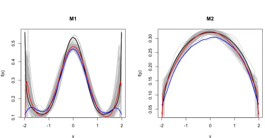
Figure 2.1 Marginal estimated curve plot for Beta-non-Beta mixture case (k1 =

10, n= 800). Solid black is the true density. Solid red is the median obtained from 100 MCDE. Solid blue is the median obtained from 100 KDE. Gray curves are each one of 100 MCDE. . . 25 Figure 2.2 Mariginal cdf MCDE estimate (black), KDE estimate (blue) and

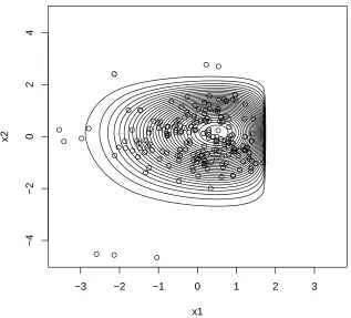
empirical cdf (red) . . . 27 Figure 2.3 Joint standardized data and contours of estimated density . . . . 28

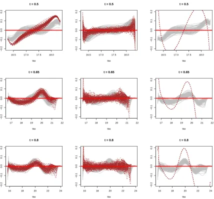
Figure 3.1 Density estimation result whenµ,{φk, λk}k2=1,{Zi}Ii=1 are all known.

First column compares MCDE with KDE. Second column compares MCDE with ECDF. Each row corresponds to a different t0. . . 44

Figure 3.2 Density estimation result for BLUP-S1: regular and dense. First column compares MCDE with KDE. Second column compares MCDE with ECDF. Third column compares MCDE with NORM. Each row corresponds to a different t0. . . 46

Figure 3.3 Density estimation result for BLUP-S2: irregular and dense. First column compares MCDE with KDE. Second column compares MCDE with ECDF. Third column compares MCDE with NORM. Each row corresponds to a different t0. . . 47

Figure 3.4 Density estimation result for BLUP-S3: regular and sparse. First column compares MCDE with KDE. Second column compares MCDE with ECDF. Third column compares MCDE with NORM. Each row corresponds to a different t0. . . 48

Figure 3.5 Density estimation result for BLUP-S4: irregular and sparse. First column compares MCDE with KDE. Second column compares MCDE with ECDF. Third column compares MCDE with NORM. Each row corresponds to a different t0. . . 49

Figure 3.6 Density estimation result for BETA-EBLUP-S1: regular and dense. First column compares MCDE with KDE. Second column compares MCDE with ECDF. Third column compares MCDE with NORM. Each row corresponds to a different t0. . . 50

Figure 3.7 Density estimation result for BETA-EBLUP-S4: irregular and sparse. First column compares MCDE with KDE. Second column compares MCDE with ECDF. Third column compares MCDE with NORM. Each row corresponds to a different t0. . . 51

(11)

Figure 3.9 Density estimation result for NORM-EBLUP-S4: irregular and sparse. First column compares MCDE with KDE. Second column compares MCDE with ECDF. Third column compares MCDE with NORM. Each row corresponds to a differentt0. . . 54

Figure 3.10 Trajectories for all subjects. The horizonal axis is wavelength at which responses are measured. The vertical axis is absorbence. Red curve represents fitted mean function. . . 56 Figure 3.11 Estimated eigenfunctions . . . 57 Figure 3.12 estimated FPC score from the first two dimensions . . . 58 Figure 3.13 Marginal score histogram. Standard normal density function is

shown in red. . . 59 Figure 3.14 Estimated CDF using four methods . . . 59

Figure 4.1 Eigenfunction estimation. True function is drawn in red. Row 1 to 4: binary cluster 1, binary cluster 2, continuous cluster 1, continuous cluster 2. Column 1 to 2: eigenfunction 1 and 2 within each cluster. 85 Figure 4.2 Eigenfunction estimation. Bias of absolute value. Row 1 to 4: binary

cluster 1, binary cluster 2, continuous cluster 1, continuous cluster 2. Column 1 to 2: eigenfunction 1 and 2 within each cluster. . . . 86 Figure 4.3 Left: binary eigenvalue bias. Middle: continuous eigenvalue bias.

Right: measurement error variance bias for continuous cluster 1 and 2. 87 Figure 4.4 Latent score covariance bias (absolute value). Top left: binary cluster

1, continuous cluster 1. Top right: binary cluster 2, continuous cluster 1. Bottom left: binary cluster 1, continuous cluster 2. Bottom right: binary cluster 2, continuous cluster 2. . . 88 Figure 4.5 Boxplots of MAPE. . . 89

Figure A.1 Beta-Beta mixture, case 1 (pf2 = 8), from first row to third row,n =

500,800,1000. . . 102 Figure A.2 Beta-Beta mixture, case 2 (pf2 = 16), from first row to third

row,n = 500,800,1000. . . 103 Figure A.3 Beta-Beta mixture, case 3 (pf2 = 32), from first row to third

row,n = 500,800,1000. . . 104 Figure A.4 Beta-non-Beta mixture, case 1 (k1 = 10), from first row to third

row,n = 500,800,1000. . . 107

(12)

Figure B.2 FPCA results for regular and dense design. Scores are generated

from a Beta-Beta mixture. . . 113

Figure B.3 FPCA results for irregular and sparse design. Scores are generated from standard bivariate normal. . . 114

Figure B.4 FPCA results for irregular and sparse design. Scores are generated from a Beta-Beta mixture. . . 115

Figure B.5 DTI trajectories with estimated mean function in red . . . 116

Figure B.6 Estimated eigenfunction . . . 117

Figure B.7 estimated FPC score from the first two dimension . . . 118

Figure B.8 Marginal score histogram. Standard normal density function is shown in red. . . 118

(13)

CHAPTER

1

INTRODUCTION

The structure of the rest of this thesis is as follows. Chapter 2 introduces a density estimation method with some specific moment constraints. The motivation for this chapter can be traced to functional principal component analysis (FPCA), which is a dimension reduction technique frequently used for functional data or longitudinal data. By the well known Karhunen-Loeve theorem, the random effect terms resulted from FPCA, also known as functional principal component scores, satisfies certain moment conditions. In particular, their marginal means are zero and their covariance matrix is the identity matrix. The key is that if we get to know the density or distribution function of those latent random effects, we are able to do any probabilistic inference on the observed response variable. In typical FPCA settings, for simplicity reason people assume that scores are normally distributed, which make probabilistic inference trivial. Instead we not only release normality assumption, but also consider the dependence across scores. Such consideration leads to our mixture model based density estimation method.

With the moment constraint density estimation method developed from Chapter 2, in Chapter 3 we apply it directly to functional principal component analysis. We review some popular existing methods for FPCA and we rely on existing software to carry out FPCA in our simulation study, but we focus on the density estimation part afterwards.

(14)

(15)

CHAPTER

2

ON MODELS AND ESTIMATION OF UNCORRELATED

DEPENDENT DATA USING CONSTRAINED EM

ALGORITHM

2.1 Introduction

Statistical estimation of a multivariate density function subject to a given set of moment restrictions has received much attention in recent literature. One of the primary motivations of this paper stems from Functional Principal Component Analysis (FPCA), in which a functional response Y(t) with _E[Y2(t)<∞] is approximated by a (truncated) Karhunen-Lo´eve Expansion (KLE) (Karhunen, 1947; Loeve, 1978): Y(t) = PK

k=1

√

λkφk(t)Zk. Here

{λk}K

k=1 are eigenvalues and {φk(t)}Kk=1 are corresponding eigenfunctions. (Z1, . . . , ZK)

(16)

dependence measures, and thus standard normal may not be an appropriate model for such joint density. In this paper we propose a flexible joint density model for (Z1, . . . , ZK) that satisfies all required moment conditions of the scores of KLE and also develop a computationally efficient method to estimate such a model based on observed data.

We discuss a variety of dependence measure and their significance in our context. Specifically we are interested in necessary and sufficient condition of independence. While Pearson’s correlation has been widely used by statisticians as a dependence measure of linear relationship between two random variables, zero Pearson’s correlation is not a necessary and sufficient condition of independence. Likewise, rank correlation measures, such as Spearman’s rho and Kendall’s tau (Annis, 2006), can be zero even when the random variables are dependent. This limitation prevents these three correlation coefficients to be an universal choice of dependence measure, and thus it is desirable to use alternative measures. Kullback-Leibler divergence (KLD) and distance correlation (Kullback & Leibler, 1951; Sz´ekely et al., 2007; Sz´ekely & Rizzo, 2013) appear to be ideal candidates of dependence measure especially when a joint density is used because zero KLD or distance correlation implies independence, and vice verca.

For two probability distributions, KLD is defined as

Dkl(f, g) =

Z Z

R2

log

f(x1, x2)

g(x1, x2)

f(x1, x2)dx1dx2, (2.1)

wheref(x1, x2) andg(x1, x2) are the pdf of each distribution. This quantity can be used to

measure the dependence of a joint distribution if we setg(x1, x2) to be the product of the

marginal densities corresponding to the joint distribution (Ebrahimi et al., 2010). That is, g(x1, x2) = f1(x1)f2(x2),where f1, f2 are the marginal pdf. If the joint distribution is

independent, then f(x1, x2) =f1(x1)f2(x2) and thus KLD is zero. Conversely, if KLD is

zero, then the log term in the integrand must be zero almost everywhere, which implies independence. In other words, a non-zero KLD value indicates that the distribution is dependent. Several other measures of dependence based on copula can be found in Joe (2014).

(17)

Introduced by Rosenblatt (1956) and Parzen (1962), kernel density estimation (KDE) is the most widely used nonparametric density estimation method. In the two dimen-sional case, suppose {(Xi1, Xi2)}ni=1 are independently and identically distributed random

variables arising from a continuous density function f(x1, x2), then the KDE can be

constructed as

ˆ

fn(x1, x2) =

1 nh1h2

n

X

i=1

K

Xi1−x1

h1

K

Xi2 −x2

h2

(2.2)

where K is a kernel function satisfying K(u) ≥ 0 and R K(u)du = 1. h is called the smoothing parameters, also known as bandwidth. Under some mild regularity conditions, KDE has been shown to be pointwise and uniformly consistent (Scott, 2015; Wasserman, 2006; Tsybakov, 1997; Silverman, 1978). The major disadvantage of KDE is that it is not designed to satisfy a given set of moment restrictions.

Another type of density estimator, introduced by Vitale (1975), uses Bernstein poly-nomial (Bernstein, 1912). The n+ 1 Bernstein basis polynomials of degree n are defined as

bv,n(x) =

n v

xv(1−x)n−v, v = 0, . . . , n, x∈[0,1]

For any continuous function G on the closed interval [0,1], the associated Bernstein polynomial is given by

Bn(x, G) = n

X

v=0

Gv n

bv,n(x).

Lorentz (1986) showed that as the degree of polynomial goes to infinity, the approximation converges uniformly to the true function. For any continuous distribution functionF with support [0,1], Vitale (1975) suggested using Pn

v=0Fˆ

v n

(18)

beta mixture model without moment constraint. One advantage of preferring a mixture model to kernel density estimator is that, as noted in section 3 of Guan (2016), model selection is easier than that of kernel density estimator. Refer to McLachlan & Peel (2005) for a review on finite mixture models. Eloyan & Ghosh (2011) presented a mixture model with moment constraints using normal mixture for the univariate density estimation scenario.

In this paper, we extend the methods described by Guan (2016) and Eloyan & Ghosh (2011) and present a new bivariate density estimation method with moment constraints using mixture of Beta density function. We implement our method via EM algorithm. Dempster et al. (1977) proposed the EM algorithm and showed that the algorithm converges to the maximum-likelihood estimate under some regularity conditions. The maximization in the M-step is implemented using Frank-Wolfe algorithm. Illustrated by Jaggi (2013), this method is shown to be numerically stable. The idea of two-step estimation is inspired by Dou et al. (2016), in which they estimated a Baker distribution.

We illustrate the numerical performance of our estimator using several simulated data scenarios. Behboodian (1990) introduced a general way to construct dependent uncorrelated bivariate random variable, which will be used in our simulation study. Turnbull & Ghosh (2014) illustrated a way to create skewed half circle distribution.

The paper is organized as follows. Section 2.2 describes the proposed moment con-strained mixture model. Section 2.3 provides detailed step for the concon-strained EM algorithm. Simulation results on the performance of the proposed estimates are shown in Section 2.4. Section 2.5 gives a real data example. And finally, section 2.6 draws a conclusion and presents some final remarks.

2.2 Model Description

Suppose we observe n independently and identically distributed (i.i.d) bivariate random variable (Xi, Yi) ∼ f(x, y) where f(x, y) is the true joint density generating the data and further assume that _Ef[X] = R R

xf(x, y)dxdy = 0,_Ef[Y] = R R

yf(x, y)dxdy = 0,_Ef[X2_{] = 1,}

Ef[Y2] = 1,Ef[XY] = 0. Our goal is to obtain an estimator ˆf(x, y) of f(x, y) that also satisfies _E_fˆ[X] = E_fˆ[Y] = E_fˆ[XY] = 0 and E_fˆ[X2] = E_fˆ[Y2] = 1. To

(19)

E_fˆ[X] =E_fˆ[Y] = 0. To estimate this joint density while also accommodating all marginal

and joint moment conditions, we propose the following nonparametric mixture model, for N1, N2 = 2,3, . . .:

ˆ

fN1,N2(x, y) = N1

X

j=1

N2

X

k=1

ωj,kbN1(x|j, a, b)bN2(y|k, c, d), (2.3)

where

bN(x|j, a, b) = N b−a

N −1 j−1

x−a b−a

j−1

1− x−a

b−a

N−j

, a≤x≤b, j= 1, . . . , N

(2.4) is the density function of a location scaled transformation of Beta density. Various aspects of linear transformation of Beta distribution and reparametrization can be found in the Appendix. ωjks are positive weight parameters. To make (2.3) to be a valid density function, the sufficient condition PN1

j=1

PN2

k=1ωjk = 1 shall be imposed. N1 andN2 act as

smoothing parameters that determine the number of components in the mixture and will be suitably chosen to ensure the smoothness of the estimated densities. Also notice that if we choose _eωjk = f(a+ (b−a)(j −1)/(N1−1), c+ (d−c)(k−1)/(N2−1)) and ωjk =

e

ωjk/PN_j₌₁1 PN_k₌₁2 ωejk, then it is well known that||fˆN1,N2−f||∞ = sup x∈[a,b],y∈[c,d]

|fˆN1,N2(x, y)− f(x, y)| →0 as min{N1, N2} → ∞ (Tenbusch, 1994). Various rates of convergence are

also available based on the chosen metric of convergence and smoothness off(·). Our goal is to estimate true density functiont subject to a given set of moment constraints, which in turn boils down to estimating the weights subject to linear equality constraints.

If the support of the bivariate random variable is [0,1]×[0,1], then these location and scale parameter in the Beta density can be eliminated. This can be achieved by simple linear transformation U = (X−a)/(b−a), V = (Y −c)/(d−c). Based on (2.3), the model for (U, V) is

ˆ

fU,V(u, v) = N1

X

j=1

N2

X

k=1

ωjkbN1(u|j)bN2(v|k), (2.5)

where

bN(u|j) =N

N −1 j−1

(u)j−1(1−u)N−j,0≤u≤1. (2.6)

(20)

can obtain the estimator for fX,Y by using the transformation ˆfX,Y(x, y) = [(b−a)(d− c)]−1_f_ˆ

U,V x_b₋−_aa,y_d−₋c_c

. Notice that ˆfU,V(u, v) will satisfy a set of moment conditions that will be equivalent to those required to be satisfied by ˆfX,Y(x, y).

Now we investigate whether (2.3) can accommodate all dependence and moment conditions. It is clear that the density in (2.5) cannot be factored into product of functions of u and v unless we choose ωjk = θjθk for some θj’s, and hence the model is capable of estimating all levels of dependence structures. Then it remains to be shown that this model is able to capture all moment constraints. SincebN1(x|j) andbN2(y|k) are free from parameters, all moment conditions translate to conditions on N1, N2 and ωjk. Therefore,

the next two questions to be answered are: (a) Under what condition(s) on the weight parameter ωjk will all the moment constraints be satisfied? and (b) Can those conditions be satisfied simultaneously?

Starting from the moment constraints and plugging in the model form, one can reach conditions on ωjk in terms of moments of Beta distribution. Those expressions can be useful if we want to apply direct maximum likelihood estimation. However, since we choose to apply the EM algorithm, the conditions on ωjk shall be derived alternatively.

2.3 Estimation Procedure

(21)

Given (Xi, Yi)

Estimate margin 1

Estimate margin 2

Estimate joint density

ˆ f(x, y) ˆ

ω(1)_, b

N1

ˆ

ω(2)_, b

N2

ˆ ωJ

2.3.1 Step One

Starting from the standardized model (2.5), we integrate with respect to u and v and obtain marginal densities. For u, v ∈[0,1]:

fU(u) = N1

X

j=1

ω_j(1)bN1(u|j), fV(v) = N2

X

k=1

ω(2)_k bN2(v|k), (2.7)

where

ω_k(2) = N1

X

k=1

ωjk, k= 1, . . . , N2, ω (1)

j = N2

X

j=1

ωjk, j = 1, . . . , N1. (2.8)

We illustrate how to obtain an estimator for one of the marginal densities, say ˆfU; the process for ˆfV is identical and is omitted here. For convenience we denoteN1 ≡N and

ω_j(1) ≡ωj in this subsection.

Before describing the EM algorithm, we have to know how the moment conditions translate to conditions on the parameter. Originally we have_E[X] = 0 and Var(X) = 1. Linear transformation to U brings_E[U] =−a/(b−a) and Var(U) = 1/(b−a)2_.

Denote ω ={ωj}Nj=1. From the moment constraints onU, we can further obtain the

condition on ω. Imagine a latent random variable Z that labels which beta distribution is used to generate U. In other words,U|(Z =z)∼Beta(z,1 +N −z) and P(Z =j) = ωj, j = 1, . . . , N1. Now, from the mean condition,

E[U] =E[E[U|Z =z]] = E

Z N + 1

=

PN

j=1jωj

(22)

we have

N1

X

j=1

jωj =

a(N + 1)

a−b ≡T1. (2.10)

The variance condition,

Var(U) = Var(_E[U|Z =z]) +_E[Var(U|Z =z)] = E[Z

2_]₋_T2 1

(N + 1)2 +

(N + 1)T1−E[Z2]

(N + 1)2_(N_{+ 2)}

(2.11) leads to

N

X

j=1

j2ωj =

T₁2− N+ 1

N+ 2T1+

(N + 1)2

(b−a)2

N + 2

N + 1 ≡T2. (2.12)

If we let

R =



 

1 1 · · · 1

1 2 · · · N

1 22 · · · N2





 and r =

   1 T1 T2  

, (2.13)

then the equality constraints can be written in matrix form as Rω =r. We will show later that the parameter space defined by this constraint is non-empty.

A constrained EM algorithm is used to estimate ω for a given basis number N. To start with, for each observed value Ui,1≤i≤n, we introduce latent random variable Zi such that

P(Zi =z) =ωj, Ui|(Zi =z)∼g(u|Zi =z) =b(u|z, N+ 1−z), (2.14)

Here g is used to denote the conditional distribution of Ui given Zi. This allows us to write our log-likelihood function in terms of the joint distribution of ui, zi, also known as the full log-likelihood. It is given by

`(ω) = n

X

i=1

log{g(ui|ω)}= n X i=1 log ( X zi

g(ui, zi|ω)

)

. (2.15)

(23)

current iterateω(t)_{, such that}_Q(_ω|ω(t)₎_≤_`(_ω_{) for all} _θ_and_Q(θ(t)_|_θ(t)_{) =}_`(θ(t)_{). In other}

words, Qnot only serves as a lower bound to ` but also tangent to` at θ(t)_{. To construct}

such Q, we introduce a probability distribution pi(zi) on Zi that is to be determined shortly. We also take advantage of Jensen’s inequality to construct this lower bound. This leads to `(ω) = n X i=1 log ( X zi

pi(zi)

g(ui, zi|ω) pi(zi)

) ≥ n X i=1 X zi

pi(zi) log

g(ui, zi|ω) pi(zi)

. (2.16)

As we require that the minorizing function tangent to the log-likelihood function at ω[t], g(ui,zi|ω)

pi(zi) needs to be a constant with respect to zi. This can be accomplished by setting

pi(zi) to be the conditional distribution of zi given ui and ω[t]. So

pi(zi) =P(Zi =z|ui,ω[t]) =

g(Zi =z, ui|ω[t]) g(ui|ω[t])

= ω

[t]

z g(u|Zi =z)

PN

j=1ω [t]

j g(u|Zi =j)

=pc(zi|ui,ω[t]). (2.17) Pluggingpc(zi|xi) into (2.16) leads to

Q(ω|ω[t]_{) =}

n

X

i=1 X

zi

pc(zi|ui,ω[t]) log

g(ui, zi|ω) pc(zi|ui,ω[t])

= n X i=1 N X j=1

pc(j|ui,ω[t]) log{ωj}+constant.

(2.18)

The last equation follows by grouping any term that does not depend on ω to a constant term. Thus E-step is completed.

The M-step is essentially an optimization problem with linear constraints. So we need to show the existence of optimal solution. Before that we need to give condition on N that guarantees a nonempty feasible region, which is discussed in the following theorem.

Theorem 2.3.1. Let R and r be defined as in (2.13) and let C={ω|Rω =r,ω>0}. If ₍a_a2₋+1_b₎2 ≤1, then there exists an N? >3 such that for all N ≥N?, C is nonempty.

Proof. First of all, we have three equality constraints, which means number of parameter N ≥3. Second, if the first condition PN

j=1ωj = 1 is satisfied, then 1 ≤

PN

(24)

holds, which means 1≤T1 ≤N. This leads to

1 N + 1 ≤

a a−b ≤

N N + 1.

In other words, if N is sufficiently large, then the first two conditions can be satisfied simultaneously because 0≤a/(a−b)≤1 for a <0< b. Now it is desired to check if the third condition can also be satisfied for sufficiently large N. Plugging in T1 into the third

condition leads to

1≤ a

2_(N _{+ 1)(N} _{+ 2)}

(a−b)2 −

a(N + 1) a−b +

(N + 1)(N + 2) (b−a)2 ≤N

2_.

If we divide this expression by (N+ 1)(N+ 2) and letN → ∞, then the left term goes to 0 and the right term goes to 1. The middle term results into a2_{+ 1/(a}₋_b)2_{. So the first}

inequality holds regardless of the value of a, b. However, whether the second inequality holds depends on a2+ 1/(a−b)2. If a2+ 1/(a−b)2 ≤1 holds, then for sufficiently large N, all three conditions hold.

Remark 2.3.1. In the case of symmetric distribution, i.e. a=−b, if b ≥1/√3, then the feasible region is nonempty for sufficiently large N. Note that for any random variable U ∈[0,1], Var(U) =_E[U2]−_E2_[U_]_≤

E[U]−E2[U] =E[U](1−E[U])≤1/4. This means 1/(a−b)2 ≤ 1/4 and b −a ≥ 2. So if a = −b then the feasible region is nonempty for sufficiently large N. All simulation studies illustrated in this paper use symmetric distribution, but the method is applicable to non-symmetric marginal distributions as well.

We prove in the next theorem the existence of optimal solution.

Theorem 2.3.2. Let Q(ω|ω[t]₎ _{be defined as in (2.18) and} _R_,_r _{be defined as in (2.13).}

Let C={ω|Rω =r,ω ≥0}. Then the optimization problem

max

ω Q(ω|ω

[t]₎

subject to Rω =r, ω≥0.

(2.19)

(25)

Proof. We consider the equivalent minimization problem:

min

ω −Q(ω|ω

[t]

)

subject to Rω=r, ω≥0.

First of all, the set C is a convex set because if ω1, ω2 ∈ C, then for any α ∈ [0,1],

R(αω1+ (1−a)ω2) =αRω1+ (1−α)Rω2 =αr+ (1−α)r=r. And if ω1 >0, ω2 >0,

then αω1+ (1−α)ω2 >0.

Second, we will show that the negative objective function −Q(ω|ω(t)_{) is convex. Let}

aj =

Pn

i=1pc(j|ui,ω(t)) be the coefficient of log{ωj}in (2.18). Sinceaj is the sum of density evaluation, they all must be positive. −Q(ω|ω(t)_{) is twice continuously differentiable over}

Cand the Hessian is given by



     

a1 ω2

1 0 · · · 0

0 a2 ω2

2 · · · 0 ..

. . .. ... 0 · · · aN

ω2

N



     

.

Since this is a diagonal matrix and all diagonal elements are positive, this matrix is positive definite. So −Q(ω|ω(t)_{) is strictly convex. And therefore the optimal solution is}

unique.

Remark 2.3.2. The condition that ω6= 0 can be enforced by replacing the constrained set

Cby Cε ={ω|Rω =r,ω ≥ε}.

As we have shown, this optimization problem is convex because we are maximizing a concave function over a convex set. So the Karush-Kuhn-Tucker (KKT) conditions are necessary and sufficient. We implemented the optimization using Frank-Wolfe method (Frank & Wolfe, 1956), for which convergence results are also established. Based on our study, this method provides more stable and efficient result than Lagrange-Multiplier method, which is used in similar setting in Dou et al. (2016) and Eloyan & Ghosh (2011). Recall that there are two iteration going on. The outer one being the EM iteration and the inner one being the M-step. Notice that ω[t]_≡ _{current value at EM iteration}_{t. Let}

ω[t,0] ₌_ω[t] _{to be the starting value of the M step at EM iteration} _{t. Denote} _Q(_ω|ω[t,0]₎

(26)

evaluate the gradient of the objective function: ∇Q(ω[t,k]_|ω[t,0]_{). Then we minimize the}

inner product <ω,∇Q(ω[t,k]_|ω[t,0]₎_>_{with respect to the constraints} _Rω ₌_r _{via linear}

programming and obtain optimal value ω∗. Then we update using the formula

ω[t,k+1]= kω

[t,k]

k+ 2 + 2ω∗

k+ 2

The algorithm should finally converge at iteration K, and then we would use this value to prepare for the next iteration in the outer EM loop. The whole process is summarized in Algorithm 1. The convergence criteria for the outer EM loop is that the absolute difference between two consecutive log-likelihood values is sufficiently small.

Algorithm 1 Application of Frank-Wolfe to the M step

procedure _{frank wolfe}(ω[t,0] _∈_C₎

for k ←0 to K do

Compute ω∗ = arg min_ω∈C<ω,∇Q(ω[t,k]|ω[t,0])>

Set ω[t,k+1]₌ kω[t,k] k+2 +

2ω∗

k+2

return ω[t,K]

The issue that has yet to be discussed is the choice of starting value in the EM algorithm. We first tested minimum norm solution with respect toRω =rand found that it may not work as it does not guaranteeω 6=0. Three alternative choices are estimator based on the (i) empirical cumulative distribution function (ECDF)Fn, defined as ωj = Fn _Nj

−Fn j

−1

N

, (ii) uniform weight, defined as ωj = _N1, and (iii) arg minω∈_RN{||Rω−r||2₂} with respect

to ω>0. All of these satisfy the inequality constraint and the last one also satisfy the equality constraint. Nevertheless, they all lead to convergence of the EM algorithm. In practice, the first method is recommended as default and is used in our simulation study.

(27)

Mises statistic, can be found in Stephens (1976). In our method, N is determined by the following way. Babu et al. (2002) gives a bound, namely 2 ≤ N ≤ n/log(n), for the basis number in which the Bernstein type estimator achieves strong consistency. We adapt this bound and set the possible values of N to be in the set N = {4na_{, a} ₌ 0,0.1,0.2, . . . ,0.5}, with rounding applied if necessary. Starting from the smallestN, we obtain the corresponding estimator ˆω and conduct a Kolmogorov-Smirnov test with the null hypothesis that the observed data comes from ˆf. If the p-value from the test is sufficiently large, then the current N is selected. If not, then we continue to the next N and redo this process. If the p-value is always less than the threshold, then N is taken to be 4n0.5 _{as a stopping criteria. In our study, the p-value threshold is set to 0.3, but other}

choises (>0.15) are also possible. This method is used in our simulation study and is proven to work well, but in real applications, researcher may set a smaller increment on N. This process is summarized in Algorithm 2.

Algorithm 2 Determine Basis Number

procedure get basis number(p-value threshold p0 >0.05)

for α ←0.0 to 0.5 by 0.1 do

Set N = 4nα

if No feasible solution ˆω at current N then

pass

else

Conduct K-S test withH0 :F =FN and HA:F 6=FN

Record p-valuepN from the K-S test

if pN > p0 or α= 0.5 then

return Basis number N

2.3.2 Step Two

Once we obtain the marginal estimator{Nb1,ωˆ1,Nb2,ωˆ2}, we may go forward and estimate

(28)

original support [a, b]×[c, d] as ˆfX,Y(x, y) and the estimator on the standardized support [0,1]×[0,1] as ˆfU,V(u, v). The relationship between them is

ˆ

fX,Y(x, y) =

1 (b−a)(d−c)

ˆ fU,V

x−a b−a,

y−c d−c

. (2.20)

As the estimator from step one is based on standardized margins, we will keep focusing on the standardized joint estimator. The form of ˆfU,V(u, v) should be as follows:

ˆ

fU,V(u, v) =

b

N1

X

j=1

b

N2

X

k=1

ωjkb(u|j)b(v|k). (2.21)

Here the parameter to be estimated isωJ ={ωjk}only, since basis number determination is not needed in this step.

Now we need to consider the constraints. Since we have already taken care of marginal mean and variance condition in step one, we may inherit such information from the estimators ˆω1 and ˆω2. We would also directly use the basis number Nb1 and Nb2. And

therefore we have the following conditions on ωJ.

b

N1

X

j=1

ωjk = ˆω_k(2), k = 1, . . . ,Nb2,

b

N2

X

k=1

ωjk = ˆω_j(1), j = 1, . . . ,Nb1. (2.22)

That is Nb₁+Nb₂ conditions in total, which covers all moment restrictions except zero

covariance condition. The last condition can be obtained as follows:

Cov(X, Y) = 0⇒Cov(U, V) = 0⇒ b

N1

X

j=1

b

N2

X

k=1

jkωjk =

ac(Nb₁+ 1)(Nb₂ + 1)

(a−b)(c−d) ≡T3 (2.23)

So finally we have Nb1+Nb2+ 1 conditions. Expressing ωJ explicitly as

ωJ ={ω11, ω12, . . . , ω1N2, . . . , ωN11, ωN12, . . . , ωN1N2}, (2.24)

(29)

representing a constraint, and

r2 = [ω1(1), . . . , ω (1)

N1, ω

(2)

1 , . . . , ω (2)

N2, T3] T

. (2.25)

Let C={ωJ|R2ωJ =r2,ωJ >0} be the parameter space. If 1 ≤T3 ≤ Nb₁Nb₂, then

there are infinitely many ωJ that satisfies (2.23). If (2.22) is also imposed on ωJ then there are still infinitely many ωJ because there are more variables than constraints and the last row in Rcannot be constructed by linear combination of other previous rows. So now we check if 1≤T3 ≤Nb1Nb2 can be satisfied without any other restriction possibly on

the density support. Dividing the inequality by (Nb₁+ 1)(Nb₂+ 1), we obtain

1

(Nb1+ 1)(Nb2+ 1)

≤ ac

(a−b)(c−d) ≤

b

N1Nb₂

(Nb1+ 1)(Nb2+ 1)

. (2.26)

From step 1, Nb₁ is selected such that 1/(Nb₁+ 1)≤a/(a−b)≤Nb₁/(Nb₁+ 1), and Nb₂ is

selected such that 1/(Nb₂+ 1) ≤ c/(c−d)≤ Nb₂/(Nb₂ + 1). Therefore (2.26) is satisfied

without any further restriction on Nb₁,Nb₂.

The initial value of the EM algorithm at this step is taken to beωjk = ˆω

(1)

j ωˆ

(2)

k such that both equality and inequality constraints are satisfied. Once we obtain the final estimator

ˆ

ωJ, we can get ˆfX,Y(x, y) through relationship (2.20). One interesting observation is that if the true density is indeed dependent, then one would expect that ˆωjk 6= ˆω_j(1)ωˆ(2)_k .

Remark 2.3.3. This could possibly lead to another way to measure dependence of a joint density function. For example, we can use max₁_≤_j_≤_Nˆ₁_,₁_≤_k_≤_Nˆ₂|ωˆjk − ωˆ

(1)

j ωˆ

(2)

k | or

PNˆ1

j=1

PNˆ2

k=1|ωˆjk −ωˆ

(1)

j ωˆ

(2)

k | as a measure of dependence.

2.4 Simulation Studies

(30)

2.4.1 A Class of Densities for Dependent Uncorrelated Data

In our simulation, we construct densities based on a general form introduced by Behboodian (1990). The author illustrated a way to construct dependent bivariate random variables that are linearly uncorrelated. In particular, the author proposed the following model. Let f1, f2, g1, g2 be univariate densities with meanµ1, µ2, ξ1, ξ2, variance σ12, σ22, τ12, τ22 and

let the joint density of (X, Y) be

fX,Y(x, y) =af1(x)g1(y) + (1−a)f2(x)g2(y), (2.27)

where 0< a <1. It can be shown thatX and Y are dependent if [f1(x)−f2(x)][g1(y)−

g2(y)]6= 0. It can also be shown that X and Y are uncorrelated if Cov(X, Y) = a(1−

a)[µ1−µ2][ξ1−ξ2] = 0. These conditions lead to conditions on density means and variances,

which we provide more detail in the supplementary material.

2.4.2 Summary of Density Function

In this subsection we provide the actual density used in the simulation. Detailed derivation of those densities can be found in the Appendix.

The first type of density is called Beta-Beta mixture, wheref1, f2, g1, g2 are all based on

Beta distribution. LetB(x|α, β) be the Beta probability density function with parameter α and β. Table 2.1 lists the three cases for Beta-Beta mixture density, where k11 =

5.56, k12 = 2.93, k21 = 5.89, k22 = 2.93, k31 = 6.09, k32 = 2.93 are normalizing constant.

Note that the only difference between the three cases are the parameters of f2(x), which

controls the dependence level.

The second type of density is called Beta-non-Beta mixture, where f1 and f2 are

still based on Beta density but g1 and g2 are based on skewed half circle distribution

fHC(x) = (2/π)(x/4 + 1/2)

p

1−(x/2)2_{. Table 2.2 lists the three cases for Beta-non-Beta}

mixture density. In these three cases, the parameter in the Beta distribution, namely k1 = 10, k2 = 20, k3 = 30, control the dependence level.

2.4.3 Dependence Measure

(31)

be-Table 2.1 Specific Densities for Beta-Beta Mixture

f1(x) f2(x)

Case 1 B(x/k11+ 1/2|2,2)/k11 B(x/k11+ 1/2|8,8)/k11

Case 2 B(x/k21+ 1/2|2,2)/k21 B(x/k21+ 1/2|16,16)/k21

Case 3 B(x/k31+ 1/2|2,2)/k31 B(x/k31+ 1/2|32,32)/k31

g1(y) g2(y)

Case 1 B(y/k12+ 1/2|1,4)/k12 B(y/k12+ 1/2|4,1)/k12

Case 2 B(y/k22+ 1/2|1,4)/k22 B(y/k22+ 1/2|4,1)/k22

Case 3 B(y/k32+ 1/2|1,4)/k32 B(y/k32+ 1/2|4,1)/k32

Table 2.2 Specific Densities for Beta-non-Beta Mixture

f1(x) f2(x)

Case 4 B((x+ 2)/4|k1, k1)/4 B((x+ 2)/4|(2k1+ 3)/(4k1 −2),(2k1+ 3)/(4k1−2))/4

Case 5 B((x+ 2)/4|k2, k2)/4 B((x+ 2)/4|(2k2+ 3)/(4k2 −2),(2k2+ 3)/(4k2−2))/4

Case 6 B((x+ 2)/4|k3, k3)/4 B((x+ 2)/4|(2k3+ 3)/(4k3 −2),(2k3+ 3)/(4k3−2))/4

g1(y) g2(y)

Case 4 fHC(y) fHC(−y)

cause it is challenging to analytically evaluate the double integral for our joint distribution in (2.1). In practice, we use the hcubaturefunction from the R package cubature. We approximate theoretical distance correlation by computing sampling distance correlation (n= 1000) using dcorr function from theenergy package.

We also report Spearman’s rho correlation coefficient, denoted as ρs. DenoteF(x) and G(y) as the marginal cumulative distribution functions, then the theoretical definition

of ρs is ρs = 12E[F(X)G(Y)]−3. To obtain ρs for each case, we also use numerical integration. Now we argue that several commonly used copula models, including Gaussian, Marshall-Olkins (MO) and Farlie-Gumbel-Morgenstern (FGM), are not appropriate in our setting. For the Gaussian copula, zero Pearson’s correlation indicates independence, while for MO and FGM copulae, zero Spearman’s rho indicates independence. Since our true generative model satisfy both zero Pearson’s correlation and zero Spearman’s correlation, a contradiction between correlation and dependence emerges. This contradiction prevents us from using copula models.

(32)

Table 2.3 Dependence measure for Beta-Beta mixture

Case 1 Case 2 Case 3

KLD 0.082 0.148 0.212

dcorr (n= 1000) 0.205 0.288 0.341

ρs ≈0 ≈0 ≈0

Case 4 Case 5 Case 6

KLD 0.065 0.082 0.091

dcorr (n= 1000) 0.197 0.245 0.262

ρs ≈0 ≈0 ≈0

Beta-non-Beta mixture. The dependence measure can be reflected from either KLD or distance correlation from Table 2.3.

2.4.4 Evaluation Methods

We evaluate the performance of the density estimates in two types of measure. For the first one we use the estimate of L1 difference between our estimates and the true density

both jointly and marginally. We report the average ofL1 difference from all Monte Carlo

(MC) samples and we also show boxplot of all L1 difference. The estimate of joint L1

difference is defined as follows, for the sth MC sample,

||fˆs−f||1 =

1 d1d2

I

X

i=1

J

X

j=1

ˆ

fs(xi, yj)−f(xi, yj)

, (2.28)

where I = 100, J = 100 and{(xi, yj)} creates a two dimensional grid on the support with equally spaced interval and d1, d2 are the width of the interval. The formula to calculate

marginal L1 difference is very similar.

Other performance measure can be found among density estimation literature, such as mean integrated square error (MISE), a measure of L2 difference. However, MISE may

(33)

The second type is the moment bias, including mean of estimated marginal mean, mean of estimated marginal variance and mean of estimated covariance. For MCDE, the mean of estimated marginal mean for first margin is

1 S S X i=1   

(ˆbi−ˆai)

b

Ni1

X

j=1

b

Ni2

X

k=1

ˆ ωijk

PNbi1

j0₌₁j0ωˆ_ij0

b

Ni1+ 1

+ ˆai







, (2.29)

the mean of estimated marginal variance for first margin is

1 S S X i=1   

(ˆbi−ˆai)2

b

Ni1

X

j=1

b

Ni2

X

k=1

ˆ ωijk

A−B2

(Nb_i₁+ 1)2

+ (Nbi1 + 1)B−A (Nb_i₁+ 1)2(Nb_i₁ + 2)

!   (2.30) where A= b

Ni1

X

j0₌₁

j02ωij0, B =

ˆ

ai(Nb_i₁+ 1)

ˆ ai−ˆbi

(2.31)

and the mean of estimated covariance is

1 S

S

X

i=1

(ˆai−ˆbi)2(ˆci −dˆi)2

P P

j0k0ωˆij0_k0−PNbi1

j0₌₁j0ωˆij0PNbi2

k0₌₁k0ωˆik0

(Nbi1+ 1)(Nbi2 + 1)

. (2.32)

For KDE, the mean of estimated marginal mean for first margin is

1 S S X i=1 1 n n X j=1

Xj, (2.33)

the mean of estimated marginal variance for first margin is

1 S S X i=1 

h2₁+

1 n

n

X

j=1

X_j2− 1

n n X j=1 Xj !2

, (2.34)

and the mean of estimated covariance is

1 S S X i=1 1 n n X j=1

XjYj− 1 n n X j=1 Xj 1 n n X j=1 Yj ! . (2.35)

(34)

Since KDE is not constructed to satisfy the moment constraints, we expect to see that our method produces better result for those quantities.

2.4.5 Results

We compare our moment constrained density estimator (MCDE) with joint kernel density estimator (KDE), which is used via the R function kde2d, in which the bandwidth is chosen by the function bandwidth.nrd(), a well-supported rule-of-thumb for choosing the bandwidth of a Gaussian kernel density estimator.

2.4.5.1 Results for Beta-Beta Mixture

As shown in Subsection 2.4.2, for the Beta-Beta mixture case, three levels of dependence strength, specified by pf2 (i.e. parameter of f2(x)), are used. We generate bivariate data from three sample size settings: n = 500,800 and 1000. That counts 9 total scenarios. In each scenario, Monte Carlo (MC) sample is set to 100. Some results for n = 800 is omitted in the main text. For illustration purpose, we show the estimated density of one particular case in Figure 2.1.

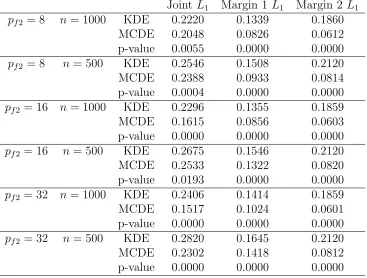
Table 2.4 shows mean L1 distance as well as p-values from testing whether there is

significant difference between the two L1 distribution. The alternative is that theL1 from

MCDE is smaller than that from KDE. Most p-values are close to zero. Addition boxplots are in the supplementary material.

Table 2.5 shows the mean of moment bias for KDE. There is no difference in terms of marginal mean bias, but KDE induces large variance bias. The result for MCDE is omitted because all numbers are close to zero. Table 2.6 shows the average number of estimated component. Since the second margin is fixed in all cases, its basis number is similar throughout. If dependence level is fixed, then number of component increases as sample size increases. If sample size increases, then number of component increases as dependence level increases.

2.4.5.2 Results for Beta-non-Beta Mixture

(35)

Table 2.4 L1 for Beta mixture case

Joint L1 Margin 1 L1 Margin 2L1

pf2 = 8 n = 1000 KDE 0.2220 0.1339 0.1860

MCDE 0.2048 0.0826 0.0612

p-value 0.0055 0.0000 0.0000

pf2 = 8 n= 500 KDE 0.2546 0.1508 0.2120

MCDE 0.2388 0.0933 0.0814

p-value 0.0004 0.0000 0.0000

pf2 = 16 n = 1000 KDE 0.2296 0.1355 0.1859

MCDE 0.1615 0.0856 0.0603

p-value 0.0000 0.0000 0.0000

pf2 = 16 n= 500 KDE 0.2675 0.1546 0.2120

MCDE 0.2533 0.1322 0.0820

p-value 0.0193 0.0000 0.0000

pf2 = 32 n = 1000 KDE 0.2406 0.1414 0.1859

MCDE 0.1517 0.1024 0.0601

p-value 0.0000 0.0000 0.0000

pf2 = 32 n= 500 KDE 0.2820 0.1645 0.2120

MCDE 0.2302 0.1418 0.0812

p-value 0.0000 0.0000 0.0000

Table 2.5 Moment Bias for Beta case

Mean1 Mean2 Var1 Var2 Cov

pf2 = 8 n = 1000 KDE -0.0000 -0.0000 1.0715 1.1333 0.0021

pf2 = 8 n= 500 KDE -0.0000 0.0000 1.4054 1.4947 -0.0066

pf2 = 16 n = 1000 KDE 0.0000 0.0000 0.7936 1.1333 0.0020

pf2 = 16 n= 500 KDE 0.0000 0.0000 1.0548 1.4947 -0.0035

pf2 = 32 n = 1000 KDE -0.0000 -0.0000 0.5363 1.1333 0.0023

pf2 = 32 n= 500 KDE 0.0000 0.0000 0.7154 1.4947 0.0025

Table 2.6 Basis number information for Beta case

(N1, N2) n = 1000 n= 500

pf2 = 8 10.48,6.32 8.35,6.64

pf2 = 16 27.20,6.40 17.51,6.68

(36)

Table 2.7 L1 distance for non-Beta case

Joint L1 Margin 1L1 Margin 2 L1

k1 = 10 n= 1000 KDE 0.1849 0.1425 0.0860

MCDE 0.1737 0.1425 0.0424

p-value 0.0003 0.5032 0.0000

k1 = 10 n = 500 KDE 0.2186 0.1687 0.0966

MCDE 0.2133 0.1692 0.0501

p-value 0.1038 0.5430 0.0000

k1 = 20 n= 1000 KDE 0.2097 0.1660 0.0858

MCDE 0.2004 0.1733 0.0459

p-value 0.0143 0.9422 0.0000

k1 = 20 n = 500 KDE 0.2510 0.2011 0.0956

MCDE 0.2496 0.2113 0.0526

p-value 0.3924 0.9652 0.0000

k1 = 30 n= 1000 KDE 0.2235 0.1780 0.0845

MCDE 0.2366 0.2089 0.0482

p-value 0.9990 1.0000 0.0000

k1 = 30 n = 500 KDE 0.2683 0.2177 0.0945

MCDE 0.2668 0.2296 0.0556

p-value 0.3935 0.9705 0.0000

and 1000, respectively. That also counts 6 total scenarios. In each scenario, MC sample size is also set to 100. Some results for n= 800 is omitted in the main text.

Table 2.7 shows the mean of both joint and marginal L1 distance for non-Beta case.

The p-values results from the same test as described in Beta case. Consider dependence level k1 = 10,20, as sample size increases, MCDE tends to outperform KDE. More

boxplots results are in the supplementary material.

(37)

Table 2.8 Moment Bias for non-Beta case

Mean1 Mean2 Var1 Var2 Cov

k1 = 10 n= 1000 KDE -0.0000 0.0000 0.8028 1.1333 0.0042 k1 = 10 n = 500 KDE -0.0000 -0.0000 1.0586 1.4947 -0.0043 k1 = 20 n= 1000 KDE 0.0000 0.0000 0.5110 1.1333 0.0047 k1 = 20 n = 500 KDE -0.0000 -0.0000 0.6801 1.4947 -0.0001 k1 = 30 n= 1000 KDE 0.0000 -0.0000 0.3853 1.1333 0.0055 k1 = 30 n = 500 KDE 0.0000 -0.0000 0.5161 1.4947 -0.0009

Table 2.9 Basis number information for Beta-non-Beta case

(N1, N2) n= 1000 n= 500

k1 = 10 18.40,4.00 14.23,4.00

k1 = 20 63.36,4.00 28.97,4.00

k1 = 30 114.56,4.00 49.13,4.00

Figure 2.1 Marginal estimated curve plot for Beta-non-Beta mixture case (k1 = 10, n= 800).

(38)

2.5 Real Data Application

Here we apply our density estimation method to a real data set, which is stock price log return from S&P500. Consisting of over five hundred U.S. company stocks, S&P500 is one of the most widely used indices for domestic stock performance. Instead of looking the index performance, we focus on price change within each component. In particular, we obtain component price from four days. Let C be the total number of component in the index. Denote Pcd be the price of component c from day d, 1 ≤ c ≤ C,1 ≤ d ≤ 4. Let Xc = log (Pc2/Pc1) and Yc= log (Pc4/Pc3) be the log return of component cfrom first

two days and last two days, respectively. The difference between first two days should be equal to the difference between last two days. For example, the first two days could be chosen as Monday and Tuesday and the last two days could be Monday and Tuesday on the following week. By fitting a density on (Xc, Yc), we are able to know the relationship between current week’s stock change and next week’s stock change.

Another reason to use this data set is that it satisfies dependence and correlation assumption. For the stock price from component c, Xc and Yc cannot be independent. On the other hand, it has been shown that Corr(Xc, Yc) = 0. In practice, we may still standardize our data to have empirical zero mean, unit variance and zero correlation.

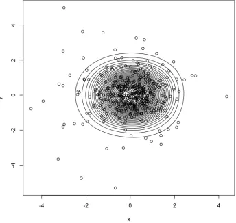
The data is obtained from The Center for Research in Security Prices (CRSP), which can be accessed by Wharton Data Research Services (WRDS). To preprocess the data, we first remove any negative price and compute log returnXcandYcas shown above. The final sample sizenis 505. The distance correlation is 0.48 and the pearson correlation is 0.51. We focus on a closed region in which most component lies, which is [−0.05,0.05]×[−0.1,0.1]. Denote then×2 sample data matrix asX. Denote the 2×1 sample mean vector and 2×2 sample variance as ¯µand V¯, respectively. We standardize our data by (X−1nµ¯T)V¯−1/2, such that it has zero mean and identity covariance matrix. The standaridized data lies mainly in the region [−4,4]×[−4,4]. The distance correlation of the standardized data is 0.08.

(39)

Figure 2.2 Mariginal cdf MCDE estimate (black), KDE estimate (blue) and empirical cdf (red)

along with empirical cdf in red. Figure 2.3 shows joint standardized data along with contours of estimated density. Both figures demonstrate the flexibility and accuracy of our estimator. Meanwhile, all moment bias have magnitude less than 10−13.

2.6 Final Comments

We have introduced a non-parametric density estimation method using Beta mixtures that is able to handle both dependence condition and moment conditions. We presented a two-step method that utilized EM algorithm in each two-step. The entire algorithm demonstrated computational stability and efficiency. R code for both estimation and simulation are available upon request for convenient implementation of our methodology. The process to generate dependent and uncorrelated data set is covered comprehensively within the simulation section. Simulation studies demonstrated power of our method that other method cannot reach.

(40)

(41)

CHAPTER

3

FUNCTIONAL PRINCIPAL COMPONENT ANALYSIS

WITHOUT GAUSSIAN ASSUMPTION ON SCORES

3.1 Introduction

Functional data consist of repeated measures of some characteristic on an individual. With the advance of modern technology, the amount of measurement per subject increases tremendously in recent years and hense such measurements can be considered as functional values for each subject. As a result, researchers are becoming increasingly interested in analyzing functional data. Functional principal component analysis (FPCA) serves as a building block of most functional data analysis. In this chapter, we propose a modeling framework that captures various distributional aspects of the stochastic process

{X(t), t∈ T }, where T ∈_Rd _{is an index set and} _Y_{(t) is a real-valued stochastic process} that is observed with errors around the true process X(t). Relatively, less attention has been paid to probabilistic inference about the X(t) process, such as calculating probabilities like P(X(t)> τ) or P(X(t2)> τ2|X(t1)> τ1) etc. for some t1, t2 ∈ T.

(42)

provided by FPCA allows us to perform probabilistic inference about Y(t), which is the focus of this chapter.

Early developments in FPCA includes Rice & Silverman (1991), James et al. (2000) and Rice & Wu (2001), from which we witness transition from mixed effect model framework to dimension reduction via FPCA. Later, Yao et al. (2005) developed methods to predict latent principal component scores, while Hall & Hosseini-Nasab (2006) investigated theoretical properties of FPCA.

The efficiency of performing FPCA depends on the denseness or sparsity of the data collection process. For a dense design, the number of observation of each subject is large and typically the observation pattern is regular, for example, equally spaced within a time frame. And all subjects have their data recorded at the same time. For a sparse design, only a few observation are recorded for each subject and recorded time can vary. In this paper, we consider both cases for our numerical illustrations.

In FPCA, the majority of data analysis, including the ones referred above, are based on the assumption that the latent stochastic process is a Gaussian Process (GP). The first advantage of this assumption is that jointly normally distributed scores automatically satisfy the moment requirement in Karhunen-Loeve Expansion (KLE) (Karhunen, 1947; Loeve, 1978). That is, the scores should have zero mean, unit variance and are uncorrelated. The second advantage is that we no longer need to model the possibly nonlinear dependence between scores because uncorrelated normal random variables imply independence. We have to emphasize that KLE theorem does not claim independence among scores when the scores are non-normally distributed. So, in some cases Gaussian assumption and/or independence assumption may be violated.

(43)

of the predicted score produced by existing methods, such as those developed by Yao et al. (2005).

Although there is hardly any work addressing the probabilistic inference about the functional data within the FPCA literature, there have been some attempts to estimate the densities of the random effects within the linear mixed effect model. Some of the notable and popular methods that have appeared in the literature are based on Gallant & Nychka (1987), which proposed a seminonparametric form of density function, abbreviated as SNP, which is able to capture a wide range of density shapes and includes normal density as a special case. Davidian (2017) introduced nonlinear mixed model using SNP. Zhang & Davidian (2001) applied SNP in linear mixed effect model. Chen et al. (2002) used SNP in generalized linear mixed effect model. Our goal in this paper is to extend some of these finite dimensional random effects based density estimation to the countably many random effects (scores) model as required in FPCA. Moreover, we attempt to estimate the joint distribution of the scores that preserves the required moment restrictions as prescribed by the KLE. This aspect of joint density estimation has rarely been addressed in existing literature.

The rest of this chapter is organized as follows. In Section 3.2 we introduce the type of data that we try to analyze and the models for such data. In Section 3.3 we provide a review of existing FPCA method and discuss how to integrate a density estimation process into FPCA that preserves the moment restrictions. In Section 3.4 we give theoretical justification of our method to show the benefit of using moment constraint density estimation. Detailed simulation results can be found in Section 3.5. We include a real data application of our method in Section 3.6. And finally, in Section 3.7 we give some final comments regarding our method as well as future directions.

3.2 Functional Model for Longitudinal Data

Consider a stochastic process{X(t) :t ∈ T } defined on an index set T. Without loss of generality, T can be set to [0,1] by using a transformation. In most practical situations we may only observe a finite sample of data points from the corrupted process Y(t) = X(t)+ε(t), whereε(t) is a white noise process. The primary goal of our study is to estimate

probability like P(X(t)∈ A) or conditional probabilities like P(X(t2)∈ A2|X(t1)∈ A1)

(44)

the data and then estimate the latent score density.

Before the advent of FPCA, Rice & Wu (2001) proposed to model X(t) as X(t) = µ(t) +hi(t), whereµ(t) is the overall fixed mean function andhi(t) is a random subject specfic function. Then µ(t) and hi(t) are parametrized using q basis functions S(t) = [s1(t), . . . , sq(t)]T as µ(t) = S(t)Tβ and hi(t) = S(t)Tγi. Here β ∈ Rq is fixed basis coefficient and γi ∈Rq are random basis coefficients with zero mean andq×q covariance matrix Γ. Expectation maximization (EM) algorithm is the typical way to carry out parameter estimation for this type of model (Dempster et al., 1977; Laird & Ware, 1982). The problem with this modelling framework is that the choice of fixed q is not flexible.

James et al. (2000) pointed out this issue and proposed a new model called low-rank model, which we will use as our modelling framework. On the population level, we have the the following model for t∈ T:

Y(t) = X(t) +ε(t) =µ(t) +

∞ X

k=1 p

λkφk(t)Zk+ε(t). (3.1)

This form is also known as Karhunen-Loeve Expansion. HereX(t) is the measurement error free term andε(t)∼ N(0, σ2_{) is the measurement error.}_{µ(t) is the fixed population mean}

function. In the infinite series expansion, {λk}∞k=1 are non-negative, fixed and decreasingly

ordered eigenvalues satisfying P∞

k=1λk<∞. and{φk(t)}∞k=1 are corresponding fixed and

mutually orthonormal eigenfunctions on the interval [0,1] that satisfiesR φk(t)φl(t)dt =δkl, δkl= 1 if k =l and δkl= 0 otherwise. {Zk}∞k=1 are called principal component scores. By

the KLE theorem, they have zero mean, unit variance and are linearly uncorrelated.Zk is independent from ε(t) for all k, but Zk1 and Zk2 can be dependent for some k1 and k2. Therefore, for some given t, the probability distribution of X(t) depends solely on the joint distribution of (Z1, Z2, . . .).

In reality, we may approximate (3.1) with a K-term truancated version:

Y(t)≈Y(K)(t) = µ(t) + K

X

k=1 p

λkφk(t)Zk+ε(t). (3.2)

Such uniform approximation is valid because for any >0, we can find a K sufficiently large such that_E[||Y(t)−Y(K)(t)||2_{] =}P∞

k=K+1λk < . Thus, we may useP(X

(K)_(t)_≤_τ)

(45)

Mercer (1909) establishes spectral decomposition of covariance kernel with respect to eigen components. By the Mercer’s Theorem, the set of eigenfunction induces a covariance kernelK(t1, t2) =P

∞

k=1λkφk(t1)φk(t2) that captures the covariance information

Cov(Y(t1), Y(t2)) for some time points t1 and t2.

Once we adopt this framework, the entire functional data curve can be viewed as the sum of a population mean curve, a few subject level random curves and a measurement error term. This is the so-called functional principal component analysis. One assumption we have to make is that the second order condition holds for Y(t), i.e._E[Y(t)2]<∞.

On the sample level, let Yi = [Y(ti1), . . . , Y(tiJi)]

T _{= [Yi}

1, . . . , YiJi]

T _for _i_{= 1, . . . , I} be the observed response of theith subject. Likewise, letµi = [µ(ti1), . . . , µ(tiJi))]

T _{be the} mean function evaluation for subject i, Φi be the eigenfunction evaluation matrix with column k equal to [φk(ti1), . . . , φk(tiJi)]

T_, _Z

i = [Zi1, . . . , ZiK]T, εi = [ε(ti1), . . . , ε(tiJi)]

T and D= diag(λ1, . . . , λK). For subject i the truncated model can be written in matrix form as

Yi =µi+ΦiD1/2Zi+εi (3.3) In the truncated form (3.3), score vectors Zis are identically and independently generated from some density functionfscore(z) =fscore(z1, . . . , zK) that satisfies E[Zk] = 0,_E[ZkZl] =δkl. Independent from Zi, εi ∼ N(0, σ2IJi) represents measurement error.

Since individual scores are realized but not observed, we cannot directly model the score density fscore(z). Instead density model can be built upon some predictor. In this

chapter, we will show in Section 3.3 how to obtain best linear unbiased predictor (BLUP) and its estimated version. More detail will be given in Section 3.3.

We take a two-stage approach to estimate the probability P(X(t) ≤ τ). First we perform FPCA and obtain estimators for mean function, eigenfunction, eigenvalue and measurement error variance: ˆµ(·),ˆλk,φˆk(·) and ˆσ2, respectively. Second we obtain joint density estimator for the latent scores: ˆfscore(·). Observing that (3.2) is a linear combination

of scores, we can now estimate P(X(t)≤τ) by

b

P(X(t)≤τ) =

Z

ˆ

µ(t)+PK k=1

√

ˆ

λkφˆk(t)zk≤τ

ˆ

(46)

3.3 Estimation Procedure

In this section we discuss estimation of all model components. First, we review existing FPCA techniques. This includes mean function and covariance function (i.e. eigenvalue and eigenfunction) estimation. Since this part is not our major focus, additional details are given in Appendix B.1. Second, we review methods of predicting functional principal component scores. Third, we show how to estimate the score density with moment constraints. And fourth, we demonstrate how to construct timewise cumulative distribution function.

3.3.1 Estimating Mean and Covariance Function

There are two major directions in terms of mean and covariance function estimation within FPCA literature. In the first direction, mean function and covariance function are estimated separately, such as in Yao et al. (2005). Once covariance function is estimated, eigenvalue and eigenfunction are obtained by solving an integral equation. In the second direction, both mean function and eigenfunction are represented by some common basis function and basis function coefficients are estimated together with eigenvalue, such as in James et al. (2000). After that, covariance function can be constructed based on Mercer’s theorem. Details are given in Appendix B.1.

3.3.2 Predicting the FPC Scores

(47)

For the numerical integration approach, we represent (3.3) in an alternative form by combining eigenvalue and score into a single random variable ξi = [ξi1, . . . , ξiK]T with ξik =

√

λkZik such that E[ξi] =0K and Cov(ξi) = D:

K

X

k=1 p

λkφk(tij)Zik = K

X

k=1

φk(tij)ξik (3.5)

and thus we have

Yi =µi+Φiξi +εi. (3.6)

By the Karhunen-Loeve Theorem, ξik =

R

{Xi(t)−µ(t)}φk(t)dt. So we can predict the scores as ˆξik =

R

{Xi(t)−µ(t)ˆ }φˆk(t)dt ≈

PJi

j=1[Yij −µ(tˆ ij)] ˆφk(tij)(tij −tij−1), where we

replace unobserved Xij with Yij and setti0 = 0.

BLUP is another way to predict the score. From (3.3), joint vector [ξ_iT,YT_i ]T has the following mean and covariance structure:

"

0K

µi

#

,

"

D DΦT

i

ΦiD ΦiDΦTi +σ2IJi

#

. (3.7)

And thus we may predict the score using BLUP (Robinson, 1991; Yao et al., 2005; Searle et al., 2009)

e

ξi =E[ξi|Yi] =DΦTi (ΦiDΦTi +σ

2_I

Ji)

−1₍_Y

i−µi). (3.8)

It was shown by Searle et al. (2009) that this predictor is unbiased in the sense that

E[ξe_i −ξ_i] = 0 and it is the best predictor in the sense that it minimizes Var(ξe−ξ_i)

among all linear predictorsξe. In practice, we use estimated best linear unbiased estimator

(EBLUP)

ˆ

ξi =DbΦb_iT(Φb_iDbΦb_iT + ˆσ2I_J_i)−1(Y_i−µ_b_i), (3.9)

which replaces true parameters with their estimated values. As mentioned in Yao et al. (2005), best linear unbiased prediction still holds when the scores are not normally distributed. Furthermore, Yao et al. (2005) show in their simulation study that such prediction is not only applicable to densely observed data but also quite robust to non-normal score. Finally, we denote Zeik = ξe_ik/

√

λk to be the predictor of Zik and denote

e

Zi = [Zei1, . . . ,ZeiK]T.Zeik can be estimated by Zbik = ˆξik/

p

ˆ

λk. We use Zb = [Zb₁· · ·Zb_I]T to

Models and Estimation Methods for Distribution of Scores for Functional Data.

ABSTRACT

DEDICATION

BIOGRAPHY

ACKNOWLEDGEMENTS

TABLE OF CONTENTS

LIST OF TABLES

LIST OF FIGURES

CHAPTER

1

INTRODUCTION

CHAPTER

2

ON MODELS AND ESTIMATION OF UNCORRELATED

DEPENDENT DATA USING CONSTRAINED EM

ALGORITHM

2.1

Introduction

2.2

Model Description

2.3

Estimation Procedure

2.3.1

Step One

2.3.2

Step Two

2.4

Simulation Studies

2.4.1

A Class of Densities for Dependent Uncorrelated Data

2.4.2

Summary of Density Function

2.4.3

Dependence Measure

2.4.4

Evaluation Methods

2.4.5

Results

2.5

Real Data Application

2.6

Final Comments

CHAPTER

3

FUNCTIONAL PRINCIPAL COMPONENT ANALYSIS

WITHOUT GAUSSIAN ASSUMPTION ON SCORES

3.1

Introduction

3.2

Functional Model for Longitudinal Data

3.3

Estimation Procedure

3.3.1

Estimating Mean and Covariance Function

3.3.2

Predicting the FPC Scores