Modeling the Martian Atmosphere at Potential Landing Sites and Regions of Notable Topography

(1)

ABSTRACT

SILVERMAN, MORGAN LINDSAY. Modeling the Martian Atmosphere at Potential Landing Sites and Regions of Notable Topography. (Under the direction of Robert H. Tolson and Gary Lackmann.)

Since the 1960’s several successful missions have been sent to Mars to gain a bet-ter understanding of the planet. In 2009, the Mars Science Laboratory (MSL) mission is scheduled to launch as part of the National Aeronautics and Space Administration (NASA) Mars Exploration Program. To assure the safety of this mission, an understand-ing of the Martian atmosphere is necessary. This is the first mission that may determine the landing site based on weather conditions. As such, potential landing sites at Terby Crater, Melas Chasma, Gale Crater, and Nili Fossae Trough were studied. Due to limited observations of Mars, the Planetary Weather Research and Forecast (WRF) Mars gen-eral circulation model was used to represent the Martian atmosphere. Model validation was conducted against Viking Lander 1, Viking Lander 2, and Mars Pathfinder data and showed that the Planetary WRF model was able to reasonably represent the Martian atmosphere.

This research is divided into two parts. The first part focuses on density, temperature, and wind profiles at each potential landing site. These profiles are used to determine the amount of variability engineers must account for in the spacecraft design specifications. All profile deviations were within the MSL design specifications. The largest deviations occurred at Terby Crater while the smallest deviations occurred at Nili Fossae Trough. It appears that the large topographic features of Hellas Basin and Valles Marineris affect the local airflow patterns around Terby Crater and Melas Chasma.

(2)

(3)

Modeling the Martian Atmosphere at Potential

Landing Sites and Regions of Notable Topography

by

Morgan Lindsay Silverman

A thesis submitted to the Graduate Faculty of North Carolina State University

in partial fulfillment of the requirements for the Degree of

Master of Science

Marine, Earth, and Atmospheric Sciences

Raleigh, North Carolina 2007

APPROVED BY:

Dr. Robert H. Tolson Dr. Gary Lackmann

Co-chair of Advisory Committee Co-chair of Advisory Committee

(4)

Biography

(5)

Acknowledgements

(6)

List of Tables

Table 1.1 Planetary and atmospheric parameters for Mars and Earth. Source: Read and Lewis (2004) . . . 2 Table 2.1 The Geophysical Fluid Dynamics Laboratory (GFDL) 40 level

vertical grid. . . 14 Table 3.1 Viking Lander 1, Viking Lander 2, Mars Pathfinder, and

(9)

List of Figures

Figure 1.1 The U.S. standard atmosphere (1976) for Earth and represen-tative temperature profiles for Mars during relatively clear con-ditions (solid line, based on Viking entry profiles [Seiff and Kirk 1977]) and during dusty conditions (dashed lines, based on Mariner 9 IRIS and Viking radio-occultation data covering the shaded re-gion [Hanel et al. 1972; Lindal et al. 1979]). Source: Zurek (1992) 3 Figure 1.2 Mass stream function (108 _kgs−1_{) during (a) northern hemisphere}

summer, and (b) northern hemisphere autumn equinox. Source: Haberle et al. (1999) . . . 4 Figure 1.3 Mars Orbiter Laser Altimeter (MOLA) topography (warmer

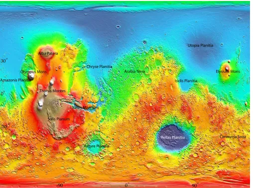
col-ors indicate higher terrain) with major surface features labeled. Source: MOLA Science Team . . . 5 Figure 1.4 Mars Orbiter Laser Altimeter (MOLA) topography (warmer

col-ors indicate higher terrain) with location of landing sites and other features of interest labeled. Source: MOLA Science Team . . . . 8 Figure 1.5 (a) Northern winter gravity wave clouds over the Kasei Vallis

region taken by the Mars Global Surveyor Mars Orbiter camera, and (b) lee waves north of Utopia Planitia taken by the Viking 1 Orbiter camera. Source: (a) Malin Space Science Systems/NASA, (b) NSSDC/NASA . . . 10 Figure 1.6 Global distribution of gravity wave potential energy per unit mass,

Ep, for all vertical wavelengths and all Lsvalues, between 10 – 30

(10)

Figure 3.1 Viking Lander 1 entry temperature (K) profile (orange) compared to Planetary WRF 333 km simulation (blue). The Martian dry adiabatic lapse rate (4.5 Kkm−1_{) is shown in green. . . .} ₁₇ Figure 3.2 Viking Lander 1 (orange) diurnal cycle compared to Planetary

WRF 333 km simulation (blue). P_scale modifications are shown in green and hypsometric pressure values in red. (a) temperature (K) versus local time in hours, and (b) pressure (mb) versus local time in hours. . . 19 Figure 3.3 Planetary WRF 333 km simulation shortwave downward radiation

(Wm−2_{) for VL1 (blue) and VL2 (red). . . .} ₂₀ Figure 3.4 Viking Lander 1 (orange) diurnal wind cycle compared to

Plane-tary WRF (blue). P_scale modifications are shown in green. (a) zonal wind component (ms−1_{) , (b) meridional wind component} (ms−1_{) , and (c) horizontal wind (ms}−1_{) versus local time in hours. 22} Figure 3.5 Planetary WRF 333 km simulation VL1, VL2, and MPF

loca-tions and regions of interest labeled. Topography is shaded and contoured at 500 m intervals. . . 23 Figure 3.6 Viking Lander 2 (orange) entry temperature (K) profile compared

to Planetary WRF 333 km simulation (blue). . . 24 Figure 3.7 Viking Lander 2 (orange) diurnal cycle compared to Planetary

(11)

Figure 3.8 Viking Lander 2 (orange) diurnal wind cycle compared to Plane-tary WRF 333 km simulation (blue). (a) zonal wind component (ms−1_{), (b) meridional wind component (ms}−1_{), and (c)} horizon-tal wind (ms−1_{) versus local time (hr). . . .} ₂₇ Figure 3.9 Mars Pathfinder (orange) temperature (K) profile compared to

Planetary WRF 333 km simulation (blue). . . 29 Figure 3.10 Mars Pathfinder (orange) diurnal cycle compared to Planetary

WRF 333 km simulation (blue). P_scale modifications are shown in green and hypsometric pressure values in red. (a) temperature (K) versus local time in hours, and (b) pressure (mb) versus local time in hours. . . 30 Figure 3.11 Mars Pathfinder (orange) and Planetary WRF 333 km simulation

(blue) horizontal wind speed diurnal cycle (ms−1_). _{. . . .} ₃₁ Figure 3.12 Zonal mean circulation during northern hemisphere summer in (a)

NASA Ames general circulation model, and (b) Planetary WRF Mars general circulation model. . . 33 Figure 3.13 Zonal mean temperature during northern hemisphere summer in

(a) NASA Ames general circulation model, and (b) Planetary WRF Mars general circulation model. . . 34 Figure 4.1 83 km simulation ratio of density standard deviation to mean

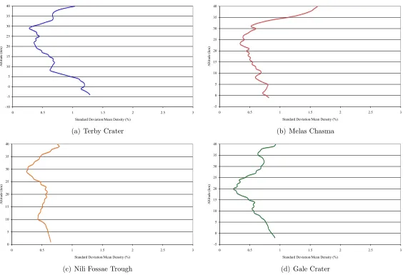
density (%) at (a) Terby Crater (1356 LT), (b) Melas Chasma (1254 LT), (c) Nili Fossae Trough (1357 LT), and (d) Gale Crater (1509 LT). . . 38 Figure 4.2 83 km simulation density to mean density ratio for 15 sols at (a)

(12)

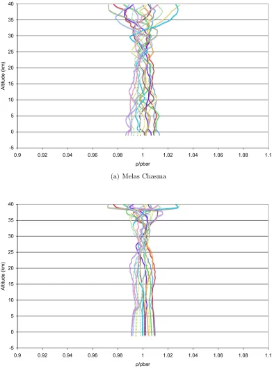
Figure 4.3 83 km simulation mean temperature (K) at (a) Terby Crater (1356 LT), (b) Melas Chasma (1254LT), (c) Nili Fossae Trough (1357 LT), and (d) Gale Crater (1509 LT). . . 41 Figure 4.4 83 km simulation temperature standard deviation at (a) Terby

Crater (1356 LT), (b) Melas Chasma (1254 LT), (c) Nili Fossae Trough (1357 LT), and (d) Gale Crater (1509 LT). . . 42 Figure 4.5 83 km simulation mean zonal wind component (ms−1_{) at (a) Terby}

Crater (1356 LT), (b) Melas Chasma (1254 LT), (c) Nili Fossae Trough (1357 LT), and (d) Gale Crater (1509 LT). . . 44 Figure 4.6 83 km simulation 15 sol time mean zonal wind at 1356 LT.

Topog-raphy is contoured at 1000 m and landing sites are represented by solid black circles. . . 45 Figure 4.7 83 km simulation zonal wind component standard deviation at

(a) Terby Crater (1356 LT), (b) Melas Chasma (1254 LT), (c) Nili Fossae Trough (1357 LT), and (d) Gale Crater (1509 LT). . 46 Figure 4.8 83 km simulation mean meridional wind component (ms−1_{) at}

(a) Terby Crater (1356 LT), (b) Melas Chasma (1254LT), (c) Nili Fossae Trough (1357 LT), and (d) Gale Crater (1509 LT). . . . 47 Figure 4.9 83 km simulation meridional wind component standard deviation

at (a) Terby Crater (1356 LT), (b) Melas Chasma (1254 LT), (c) Nili Fossae Trough (1357 LT), and (d) Gale Crater (1509 LT). . 49 Figure 4.10 83 km simulation surface wind vectors and topography (contoured

(13)

Figure 5.1 Olympus Mons horizontal wind (ms−1_{, shaded) and wind vectors} at 0004 LT. (a) surface wind and topography (contoured at 500 m, negative values are dashed), and (b) east-west vertical cross section through 18◦_{N. . . .} ₅₄

Figure 5.2 Olympus Mons east-west vertical cross section through 18◦_{N with}

W (ms−1_{, shaded) and potential temperature (K, contoured) at} (a) 2104 LT, (b) 0004 LT, (c) 0304 LT, and (d) 0604 LT. . . 55 Figure 5.3 Olympus Mons east-west cross section through 18◦_{N at 2104 LT}

with W (ms−1_{, shaded) and potential temperature (K, contoured). 57} Figure 5.4 Olympus Mons 40 km altitude horizontal wind (ms−1_{, shaded)}

and wind vectors at 2104 LT. . . 58 Figure 5.5 Olympus Mons east-west vertical cross section through 18◦_{N with}

horizontal wind (ms−1_{, shaded) and wind vectors at (a) 2104LT,} (b) 0004LT, (c) 0304LT, and (d) 0704LT. . . 59 Figure 5.6 Olympus Mons east-west vertical cross section through 18◦_{N with}

W (ms−1_{, shaded) and potential temperature (K, contoured) at} (a) 0904 LT, (b) 1204 LT, (c) 1504 LT, and (d) 1804 LT. . . 60 Figure 5.7 Olympus Mons east-west vertical cross section through 18◦_{N with}

horizontal winds (ms−1_{, shaded) and wind vectors at 1204 LT. .} ₆₁ Figure 5.8 Olympus Mons east-west cross section at 2104 LT with W (ms−1_,

shaded) and potential temperature (K, contoured) through (a) 16 N latitude, and (b) 19 N latitude. . . 63 Figure 5.9 Hellas Basin surface horizontal wind (ms−1_{, shaded) and wind}

(14)

Figure 5.10 Hellas Basin surface horizontal wind (ms−1_{, shaded) and wind} vectors at (a) 1040 LT, (b) 1340 LT, (c) 1640 LT, and (d) 1940 LT. Topography is contoured at 500 m (negative values are dashed). 65 Figure 5.11 Hellas Basin east-west vertical cross section through 40◦_{S with W}

(ms−1_{, shaded) and potential temperature (K, contoured) at (a)} 1040 LT, (b) 1340 LT, (c) 1640 LT, and (d) 1940 LT. . . 66 Figure 5.12 Hellas Basin east-west vertical cross section at 1340 LT with W

(ms−1_{, shaded) and potential temperature (K, contoured) through} (a) –40◦ _{latitude, and (b) –44}◦ _latitude. _{. . . .} ₆₈

(15)

1 Introduction

1.1 Mars Background

For several decades Mars has been in the forefront of planetary exploration research. Mars is a desirable planet to study because of its similarities to Earth and the possibility for life to have once existed. By studying the present climate of Mars, it is possible to understand the history of the planet including the nature of life. This can help provide insight into terrestrial processes and life on Earth. In 1964, the Mariner 4 spacecraft transmitted the first images of Mars. Since then there have been several successful missions, which have helped scientists gain a better understanding of Mars. As scientists learn more about the planet, new questions arise for future missions to answer. To assure the safety of future missions an understanding of the Martian atmosphere is necessary.

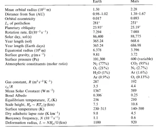
There are several distinct differences important to atmospheric modelers between Mars and Earth, in particular, their size, gravity, atmospheric composition, thermal structure, and topography. Mars rotates at approximately the same rate as Earth, where one Mars day (sol) has 24.66 Earth hours. A sol is equivalent to one Martian mean solar day, which can be divided into twenty four hours, each hour consisting of 3,699 seconds (Read and Lewis, 2004). There are 668.6 sols (686.98 Earth days) in one Martian year. The Martian atmosphere is composed of ninety-five percent carbon dioxide, with a few percent nitrogen and argon. Unlike Earth, O2 and N2 make up less than three percent of the atmosphere on Mars. Water vapor, although present on Mars, is extremely small. Only approximately 0.3 percent of the atmosphere is water vapor compared to 0–4 percent on Earth. Mars has a very thin atmosphere. This supports large diurnal ranges, because the atmosphere reacts quickly to energy gained and lost. For a complete comparison of atmospheric parameters between Mars and Earth see Table 1.1.

(16)

Table 1.1: Planetary and atmospheric parameters for Mars and Earth. Source: Read and Lewis (2004)

(17)

Figure 1.1: The U.S. standard atmosphere (1976) for Earth and representative temper-ature profiles for Mars during relatively clear conditions (solid line, based on Viking entry profiles [Seiff and Kirk 1977]) and during dusty conditions (dashed lines, based on Mariner 9 IRIS and Viking radio-occultation data covering the shaded region [Hanel et al. 1972; Lindal et al. 1979]). Source: Zurek (1992)

(18)

(a) Summer

(b) Autumn

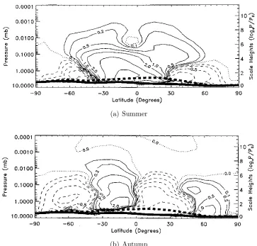
Figure 1.2: Mass stream function (108 _kgs−1_{) during (a) northern hemisphere summer,} and (b) northern hemisphere autumn equinox. Source: Haberle et al. (1999)

during the summer and winter solstice, a large cross-equatorial cell dominates (Haberle et al., 1993). Planetary waves, instabilities, and topography can also impact the zonal-mean circulation.

(19)

º

Utopia Planitia

Hellas Planitia

Olympus Mons

Chryse Planitia

Isidis Planitia

Valles Marineris Tharsis Montes

Amazonis Planitia

Elysium Mons

Argyre Planitia Alba Patera

Solis Planum

Arabia Terra

Cimmeria Terra

0º 90º

-90 0º

30º

º

-30

(20)

has an effect on the circulation of Mars, both globally and locally. Topography has been found to cause low level jets and western boundary currents (Joshi et al., 1995b; Joshi et al., 1997) as well as gravity waves (Read and Lewis, 2004; Creasey et al., 2006a; Fritts et al., 2006) and slope winds (Savijarvi and Siili, 1993). Diurnal variations can also influence the circulation. Mars has a short radiative response time due to low surface thermal inertia, which causes large diurnal ranges. Thermal tides can develop in response to this diurnal contrast (Read and Lewis, 2004; Wilson and Hamilton, 1996) as well as the development of a nocturnal planetary boundary layer (PBL) jet (Savijarvi and Siili, 1993).

The topography, circulation, composition, and thermal structure of Mars all have an impact on landing missions Because of limited in situ surface data, the general circu-lation and local effects on Mars can not be easily analysed without the use of general circulation models (GCM). The only available in situ data are from the Viking Lander 1 and 2 (1976) and Mars Pathfinder (1996) missions. These datasets still lack significant temporal (except Viking Lander 1) and spatial coverage to get a full understanding of the atmosphere though. There are several forms of remote data such as the thermal emission spectrometer (TES), infrared thermal mapper (IRTM), and others that can be used to supplement in situ data. This is why it is important for present and future missions to obtain additional scientific data. Limited data makes it difficult to validate and initialize models, causing results to be not as reliable and with the kind of precision needed.

1.2 Mars Science Laboratory Mission

(21)

pre-pare for human exploration (NASA). In 2009, the next mission in this program, Mars Science Laboratory (MSL), is scheduled to launch. MSL will contribute to the overall Mars exploration program by looking at surface radiation, planetary processes, geological and geochemical processes, as well as biological potential (JPL/NASA). In preparation for this mission, several potential landing sites have been selected to determine the best location for the rover to land. Four of these sites, Terby Crater, Gale Crater, Melas Chasma, and Nili Fossae Trough (Fig. 1.4), have been selected and classified as ”chal-lenge” sites due to their complex terrain. These sites will be studied in this research. In order to determine the feasibility of landing at these sites, the atmospheric conditions surrounding them need to be analysed. This is the first mission where the landing site may be determined based on weather conditions.

The process of landing on Mars is very complicated. The atmosphere is too thin to slow a vehicle down to an appropriate speed but is also too dense to ignore frictional heating, which occurs during spacecraft entry. The spacecraft enters the atmosphere at 125 km altitude with a speed between 4 to 8 kms−1 _{and an angle of about twelve degrees} below horizontal. When the spacecraft reaches 20 – 40 km altitude, its trajectory becomes nearly horizontal. It is within this altitude range that a significant amount of drag and heating occur on the spacecraft. Once the spacecraft reaches approximately 10 km with a speed of about Mach 2 (400 ms−1_{), a parachute is deployed, slowing the spacecraft} to the landing site. In order to achieve a successful landing, the specifications used to design the spacecraft must have little error. Through analysis of density, temperature, and wind profiles, this margin of error and design specifications are determined (R. H. Tolson 2007, personal communication).

(22)

Melas Chasma

Terby Crater

Gale Crater Nili Fossae Trough

-90º ₀º ₉₀º

30º

0º

-30º

VL1

VL2

MPF

Valles Marineris Kasei Valles→

Ares Vallis

Elysium Mons

(23)

be used to get back to the site. Temperature is important because certain sequences of events, in particular the release of the parachute, during the landing phase are activated by a specific Mach number. The Mach number,

M = u

usound (1)

is the ratio of the spacecrafts velocity to the speed of sound, where the speed of sound is proportional to the square root of temperature. The typical value for the speed of sound on Mars is 240 ms−1_{. Lastly, wind speed is critical in landing, because the spacecraft needs} to land within 10 km of the site to be considered a successful mission. The parachute is only open for about one minute before the spacecraft should land, so any error in wind speeds could cause the craft to land several hundred meters away from the target site (R. H. Tolson 2007, personal communication).

1.3 Gravity Waves

(24)

(a) (b)

Figure 1.5: (a) Northern winter gravity wave clouds over the Kasei Vallis region taken by the Mars Global Surveyor Mars Orbiter camera, and (b) lee waves north of Utopia Planitia taken by the Viking 1 Orbiter camera. Source: (a) Malin Space Science Sys-tems/NASA, (b) NSSDC/NASA

descent phase of the landing missions.

(25)

Figure 1.6: Global distribution of gravity wave potential energy per unit mass, Ep, for

all vertical wavelengths and allLsvalues, between 10 – 30 km altitude. Source: Creasey

et al. (2006a)

found increased wave activity, exhibited few inversions. Hinson and Wilson (2004) found that these inversions were caused by thermal tides. Creasey et al. (2006a) also tried to determine what wave activity was due to gravity waves and what was caused by thermal tides. After removing wavelengths greater than 10 km, they found that wave activity over the regions of Isidis Planitia, Chryse Planitia, and Amazonis Planitia was reduced by a factor of 6-8. This implied that the majority of wave activity in these regions had wavelengths longer than 10 km and were most likely thermal tides. This correlates with what Hinson and Wilson (2004) found in their study.

(26)

1.4 Research Goals

This research has two main goals. The first is designed to help select the Mars Sci-ence Laboratory mission landing site. This is the first Mars mission that may determine the landing site based on weather constraints. As such, this study will help quantify the mean density, temperature, and winds at four of the current landing site candidates and provide an estimate of the variability from the mean. Because there are limited in situ observations from Mars, numerical models must be used to quantify this informa-tion. Limited observations also pose a problem for running numerical models, because there is minimal data for model validation and initial conditions. The best method for validation is model to model comparisons of data. This research will provide data from the Planetary Weather Research and Forecast (PWRF) model, which can be compared against other global and mesoscale models to help get a more complete understanding of the atmosphere.

The second goal focuses on atmospheric disturbances generated by large topography. This is important because topographically generated gravity waves can affect the general circulation as well as impact landing missions. Very little is known about this type of phenomenon on Mars so further study is needed.

(27)

2 Methodology

For this study, numerical simulations were conducted using the Planetary Weather Research and Forecasting model (PWRF) Mars general circulation model. PWRF was developed jointly by Caltech, Cornell University, the Jet Propulsion Laboratory, and Kobe University and based on the Weather Research and Forecasting model (WRF) version 2.0.3.1. For more information on the Planetary WRF model see Richardson, Toigo, and Newman (2007). The WRF model was developed by the National Center for Atmospheric Research (NCAR) and the National Center for Environmental Prediction (NCEP), see Michalakes et al. (2004) and Skamarock et al. (2005) for further information. Two global simulations were run: 333 km grid spacing and 83 km grid spacing. The simulations used 64 x 36 and 256 x 144 grid points in the horizontal direction, respectively. The GFDL (Geophysical Fluid Dynamics Laboratory) standard 40 level vertical grid was used (Table 2.1), with a model top at 120 km. The time steps for each model run were 75 s and 30 s, respectively. Data was output at 3 hour increments. Each simulation used the Mars CO2 cycle microphysics scheme, Hourdin CO2longwave radiation scheme, LMD (Laboratoire de Meteorologie Dynamique) simplified Martian CO2 shortwave radiation scheme, LMD MGS (Mars Global Surveyor) dust radiation scheme, Monin-Obukhov surface layer scheme, Martian 12 layer subsurface diffusion land-surface scheme, and the MRF boundary-layer scheme. There was no cumulus parametrization scheme used for these simulations. Mars Orbiter laser altimeter (MOLA) 1/32 degree topography data was used.

(28)

Table 2.1: The Geophysical Fluid Dynamics Laboratory (GFDL) 40 level vertical grid. 0.0 0.19114E-04 0.4843E-04 0.97632640E-04 0.17188780E-03 0.27827270E-03 0.42686170E-03 0.62921850E-03 0.89995840E-03 0.12623930E-02 0.17457410E-02 0.23940860E-02 0.32546960E-02 0.43987000E-02 0.59048910E-02 0.78931450E-02 0.10494070E-01 0.13908130E-01 0.18350280E-01 0.24152680E-01 0.31665220E-01 0.41430940E-01 0.54009190E-01 0.70129450E-01 0.90361890E-01

0.11574140E 0.14708760 0.18574260 0.23256740 0.28731360 0.34892500 0.41752940 0.49165150 0.57069490 0.65181170 0.73338190 0.81090640 0.88163450 0.93954880 0.98118970

1.0

Sol 218 was chosen in order for the model to be spun up by the anticipated landing dates of the four potential Mars Science Laboratory sites. Four landing sites (Terby Crater [27.7435 S, 74.1137E], Melas Chasma [9.81 S, 283.62 E], Nili Fossae Trough [20.93 N, 74.35 E], and Gale Crater [4.5 S, 137.35 E]) were analysed to determine landing conditions. Two other sites, Olympus Mons and Hellas Basin, were also analysed to look at the effects of large scale topography on the atmosphere. Hellas Basin and Terby Crater were studied at a solar longitude (Ls) of 121, while the four remaining sites were studied

atLs=116. These solar longitudes were chosen based on the latitude of the site and the

time of year the mission will land. Solar longitude is the angle of the sun relative to Mars with respect to the northern hemisphere. It is used as a method used for describing the time of year on Mars, where Ls =0 is spring equinox, Ls = 90 is summer solstice, Ls=

180 is autumn equinox, and Ls = 270 is winter solstice. TheseLs values of 116 and 121

(29)

3 Model Validation

In order to test the capability of Planetary WRF (PWRF) to represent the Martian atmosphere, in situ data from the Viking Lander 1 (VL1), Viking Lander 2 (VL2), and Mars Pathfinder (MPF) missions were compared against the PWRF 333 km simulation. In situ data for VL1 was collected from 1976 through late 1982 when communications were lost. VL2 lost communication a couple years earlier. In situ data for MPF was collected from July 4 through October 7, 1997. New topography data from the Mars Orbiter Laser Altimeter (MOLA), has shown that the Viking Lander 1 vertical profile is offset by approximately one kilometer. According to Withers et al. (2002), this error causes density and pressure values to be 10–20 % too large. This error is also probably valid for the Viking Lander 2 vertical profile, but no references have been found documenting new profiles constructed for this site.

PWRF was not initialized for the conditions during 1976 or 1997. As such, PWRF can only relate conditions generally to a time of day and time of year, not to the actual conditions during the mission. This means that the diurnal patterns and vertical structure should be similar but small scale variability will not. The PWRF simulation used in all three comparisons had solar longitude (Ls) values betweenLs=115 andLs=121, northern

hemisphere summer. For an explanation of solar longitude see Chapter 2. Viking Lander 1 was compared at Ls=115 since this was the closest available modelLs value to landing

at Ls=97. Viking Lander 2 was compared at Ls=117, the true landing solar longitude,

and Mars Pathfinder was compared at Ls=121, the closest time of year to the actual

landing of Ls=142. Surface temperature, pressure, and wind data were compared for

(30)

Table 3.1: Viking Lander 1, Viking Lander 2, Mars Pathfinder, and Planetary WRF 333 km simulation local time and location of entry temperature profiles.

Local Time Latitude, Longitude

Viking Lander 1 1613 22N, 48W

Planetary WRF 1740 22.5N, 47.81W

Viking Lander 2 0949 48N, 134E Planetary WRF 0857 47.5N, 132.188E

Mars Pathfinder 0300 19N, 33W

Planetary WRF 0347 17.5N, 30.938E

throughout the day.

Surface data, except for the MPF wind data, were obtained through the Planetary Data System. The MPF wind data was obtained through communication with Jim Murphy at New Mexico State University. Entry profile data for Viking Lander 1 & 2 was taken from Seiff and Kirk (1977) and Withers et al. (2002), while entry profile data for the Mars Pathfinder was taken from Magalhães et al. (1999). Elevations at these three landing sites were estimated from 1◦ _x ₁◦ _{resolution MOLA data (D. E. Smith 2007,}

personal communication).

3.1 Viking Lander 1 & 2

On July 20, 1976 Viking Lander 1 (VL1) touched down in the Chryse Planitia region of Mars, 22 N latitude, 48 W longitude (Fig. 1.4) at an approximate height of -3.62 km relative to the geoid. Forty five days later on September 3, Viking Lander 2 (VL2) landed in the Utopia Planitia region of Mars, 48 N latitude, 134 E longitude (Fig. ??) at an approximate height of -4.44 km relative to the geoid. In order to compare the Viking Lander entry profiles to PWRF, the closest simulation times and model grid points were used for the Ls values mentioned above. See Table 3.1 for the list of local times and

(31)

Viking Lander 1 and Planetary WRF Temperature Profile

0 20 40 60 80 100 120

100 120 140 160 180 200 220 240 260

Temperature (K)

Height (km)

VL1 PWRF Dry Adiabatic Lapse Rate

Figure 3.1: Viking Lander 1 entry temperature (K) profile (orange) compared to Plane-tary WRF 333 km simulation (blue). The Martian dry adiabatic lapse rate (4.5 Kkm−1₎ is shown in green.

of 48 hours (∼2 sols) during the respective season. A period of two sols was chosen to

get a better sense of the diurnal cycle.

VL1 observations were compared with PWRF data at model level 1, in order to analyse similar elevations. The 333 km simulation did not output surface temperature and wind values to compare against. Model level 1 had an average elevation of -3.49 km at the VL1 site and an average elevation of -4.48 km at the VL2 site. The model values of terrain height at VL1 and VL2 were -3.60 km and -4.59 km, respectively. Therefore, PWRF1 is 110 m above the model topography.

3.1.1 Viking Lander 1

(32)

graph is qualitatively similar in some respects. We can not expect the profiles to have exactly the same values because the atmospheric conditions are not the same. Above 50 km, the VL1 profile has a prominent sinusoidal pattern with several inversion layers. Seiff and Kirk (1977) attribute this wave structure to strong thermal tidal oscillations. PWRF has a similar pattern. In general, both profiles appear to have two distinct regions, a lower unstable atmosphere below 50 km, and an upper stable isothermal region. The first 7 km in the PWRF profile resembles the adiabatic lapse rate. This implies that the region is well mixed and is most likely the boundary layer. Since these profiles are from the mid-afternoon, this is reasonable. The VL1 entry profile observations do not extend below 28 km, as such they can not be compared.

Figure 3.2a shows the diurnal temperature cycle at VL1. The diurnal range of PWRF is ∼10 K larger than observations, with the major anomaly occurring in minimum

tem-peratures. Opacity data at VL1, forLs=115, has values of optical depth around 0.4. This

(33)

Viking Lander 1 and Planetary WRF Diurnal Temperature Cycle

180 190 200 210 220 230 240 250

0 5 10 15 20 25 30 35 40 45

Local Time (Hr)

Temperature (K)

VL1 PWRF Pscale

(a) Temperature (K)

Viking Lander 1 and Planetary WRF Diurnal Pressure Cycle

6.5

7

7.5

8

8.5

9

9.5

10

10.5

0 5 10 15 20 25 30 35 40 45

Local Time (Hr)

Pressure (mb)

VL1 PWRF Pscale Hypsometric

(b) Pressure (mb)

(34)

Planetary WRF Shortwave Downward Radiation

-50 50 150 250 350 450 550

0 5 10 15 20 25 30 35 40 45

Local Time (hr)

Radiation (W/m

2)

VL1 VL2

Figure 3.3: Planetary WRF 333 km simulation shortwave downward radiation (Wm−2₎ for VL1 (blue) and VL2 (red).

of radiation received. Calculated values of solar insolation at VL1 and VL2 were ∼496

Wm−2 _and _∼_{458 Wm}−2_{, respectively. These are slightly higher than the model output} predicted, ∼493 Wm−2 _and _∼_{452 Wm}−2_{, which means that dust and other atmospheric} absorbers are reducing the amount of radiation received at the surface within the model. In situ data of solar radiation for these two sites was not found for comparison.

The diurnal pressure field, Fig. 3.2b, shows a wave pattern throughout the day. Ac-cording to Hess et al. (1977) the daily variation in pressure is most likely on the planetary scale and can be attributed to diurnal and semi-diurnal forcing. PWRF resembles the VL1 wave pattern well, but PWRF overestimates the pressure by approximately 2.5 mb. The reason for this discrepancy could be caused by several factors. The first factor is the amount of C02 ice in the model atmosphere. PWRF has a setting, p_scale, that controls this factor. It adjusts the P0 variable to more closely match the pressure at z=0.

(35)

per suggestion of the model developers. Once rerun the pressure decreased 1.2 mb as seen in Fig. 3.2b. Although, the adjusted pressure values are still much larger than VL1 observations. This is not likely due to terrain differences, since the VL1 elevation is below the first model level height, which would imply higher pressure values. Solving the hypsometric equation for P1, the pressure at the VL1 site,

h=zupper−zlower =

RT g ln

!_P

1

P2

"

(2)

where zupper is the height of the first model level, zlower is the VL1 height, R is the gas

constant, T is the average temperature in the layer, and P2 is the pressure at PWRF1, gives higher pressure values at P1. As previously stated, this was expected. Another factor that may contribute to the pressure difference is that the model was not completely spun up and reached steady state. It was originally stated that the model was spun up in 30 sols (C. E. Newman 2006, personal communication). More recently, it was suggested that 50 degree of Ls, approximately 105 sols, is the minimum (X. Guo 2007, personal

communication).

(36)

Viking Lander 1 and Planetary WRF Zonal Wind Diurnal Cycle -8 -6 -4 -2 0 2 4 6 8 10 12

0 5 10 15 20 25 30 35 40 45

Local Time (Hr)

W

ind Speed (m/s)

VL1 PWRF Pscale

(a) Zonal Wind

Viking Lander 1 and Planetary WRF Meridional Wind Diurnal Cycle

-8 -6 -4 -2 0 2 4 6 8 10 12 14

0 5 10 15 20 25 30 35 40 45

Local Time (Hr)

W

ind Speed (m/s)

VL1 PWRF Pscale

(b) Meridional Wind

Viking Lander 1 and Planetary WRF Horizontal Wind Diurnal Cycle

-2 0 2 4 6 8 10 12 14 16

0 5 10 15 20 25 30 35 40 45

Local Time (Hr)

W

ind Speed (m/s)

VL1 PWRF Pscale

(c) Horizontal Wind

(37)

VL2

VL1_MPF

Elysium Mons Ares Vallis

Kasei Vallis

Valles Marineris

Figure 3.5: Planetary WRF 333 km simulation VL1, VL2, and MPF locations and regions of interest labeled. Topography is shaded and contoured at 500 m intervals.

this region. This could significantly affect accurate values of model wind speeds. The horizontal wind comparison also does not match. When observations exhibit maxima, the model results show minima, and vice versa. At this course grid spacing, small scale atmospheric phenomena are also not resolved. Winds, in particular, are more affected by local effects and small scale phenomena than other variables. Adjusting the p_scale factor did not significantly affect the wind field.

3.1.2 Viking Lander 2

(38)

Viking Lander 2 and Planetary WRF Temperature Profile

0 20 40 60 80 100 120

90 110 130 150 170 190 210 230 250

Temperature (K)

Height (km)

VL2 PWRF

Figure 3.6: Viking Lander 2 (orange) entry temperature (K) profile compared to Plane-tary WRF 333 km simulation (blue).

inversions can not be directly compared. Only the general pattern and structure would be expected to be similar. Therefore, the shape of the graphs is qualitatively similar, in that in the lower part of the atmosphere temperatures decrease at the same rate until about 30 km. Above this both profiles have several inversion layers and become more stable. At the surface, a small inversion layer exists in the PWRF profile. This is most likely a remnant of the nocturnal inversion. The PWRF temperature profile is approximately one hour earlier than the observed profile. This could account for the lack of inversion in the VL2 observations.

(39)

Viking Lander 2 and Planetary WRF Diurnal Temperature Cycle

180 190 200 210 220 230 240 250

0 5 10 15 20 25 30 35 40 45

Local Time (Hr)

Temperature (K)

VL2 PWRF Pscale

(a) Temperature (K)

Viking Lander 2 and Planetary WRF Diurnal Pressure Cycle

6.8

7.3

7.8

8.3

8.8

9.3

9.8

10.3

10.8

11.3

0 5 10 15 20 25 30 35 40 45

Local Time (Hr)

Pressure (mb)

VL2 PWRF Pscale Hypsometric

(b) Pressure (mb)

(40)

there is two times more dust in the actual atmosphere at Ls = 117 at VL2 than there

was in the model, 0.39 compared to 0.17, respectively. This does not explain why VL2 has a stronger diurnal cycle than PWRF, which means that the difference is most likely attributed to the difference in model level and VL2 heights, although they are nearly the same. The opposite would be expected based on the opacity values. The diurnal pressure cycle seen in Fig. 3.7b, shows a similar wave pattern in PWRF as was seen in the VL1 diurnal pressure cycle. This pattern is less present in the VL2 observations, due to average values shown. PWRF pressure values are still consistently 2.5 mb higher than observations. Rerunning the model with p_scale=1.134, reduced the pressure 1.25 mb,

the same amount that was seen in the VL1 pressure values. The large difference that still exists between the pressure correction and observed values is likely due to incomplete model spin up as mentioned before. Solving Eq. 2, gives slightly lower pressure values as expected due to the elevation difference between PWRF1 and VL2.

(41)

Viking Lander 2 and Planetary WRF Zonal Wind Diurnal Cycle -10 -8 -6 -4 -2 0 2 4 6

0 5 10 15 20 25 30 35 40 45

Local Time (Hr)

W

ind Speed (m/s)

VL2 PWRF Pscale

(a) Zonal Wind

Viking Lander 2 and Planetary WRF Meridional Wind Diurnal Cycle

-10 -8 -6 -4 -2 0 2 4 6

0 5 10 15 20 25 30 35 40 45

Local Time (Hr)

W

ind Speed (m/s)

VL2 PWRF Pscale

(b) Meridional Wind

Viking Lander 2 and Planetary WRF Horizontal Wind Speed Diurnal Cycle

0 1 2 3 4 5 6 7 8 9 10

0 5 10 15 20 25 30 35 40 45

Local Time (Hr)

W

ind Speed (m/s)

VL2 PWRF Pscale

(c) Horizontal Wind

(42)

3.2 Mars Pathfinder

The Mars Pathfinder landed on July 4, 1997 at an approximate elevation of -3.76 km relative to the geoid in the Ares Vallis region of mars, 19 N latitude, 33 W longitude. For data comparison of local time and location to the PWRF entry temperature profile see Table 3.1. The Mars Pathfinder data was compared to model level 1, which had an average elevation of -3.17 km. The model value of terrain height at this location was -3.28 km.

Figure 3.9 shows the temperature profile from Mars Pathfinder (MPF). PWRF has a similar profile pattern to MPF observations. Below 10 km there is no MPF lander data due to spacecraft constraints on the placement of the temperature sensor (Seiff et al. 1997; Schofield et al., 1997). The PWRF simulation shows a strong inversion at the surface, representative of a nighttime profile. According to Schofield et al. (1997) the inversion at the bottom of the MPF profile is too high to be the nocturnal boundary layer thermal inversion, and that it is most likely due to water-ice clouds. This is because the minimum temperature is below the condensation temperature of water vapor for mars (∼185 K (Read and Lewis, 2004)) (Schofield et al., 1997). From 15 km to 50 km,

PWRF underestimates the temperatures, increasing in difference with increasing altitude. Above 50 km, PWRF matches the observations well until about 65 km where the MPF observations have a 2 km inversion (112–127 K) and PWRF does not. PWRF continues to decrease in temperature through this region, with a less steep lapse rate than before, until 70 km where it matches closely with the MPF observation. The discrepancy in the comparison around 80 km could be due to what Schofield et al. (1997) describe as a region of superpositioning of waves because this temperature was the lowest ever measured in the martian atmosphere at this time. Although, Schofield et al. (1997) acknowledge that the temperature at this altitude is below the CO2 condensation temperature (∼150

(43)

Mars Pathfinder and Planetary WRF Temperature Profile

0 10 20 30 40 50 60 70 80 90 100

60 80 100 120 140 160 180 200 220 240

Temperature (K)

Height (km)

MPF PWRF

Figure 3.9: Mars Pathfinder (orange) temperature (K) profile compared to Planetary WRF 333 km simulation (blue).

stated previously, these two profiles can not be expected to match identically due to the differences in the model and actual environmental conditions.

Looking at the diurnal variations the temperature pattern matches well (Fig. 3.10a). The lowest temperature occurred around 0300 LT, and the maximum temperature oc-curred around 1500 LT. The PWRF diurnal range is approximately 30 K weaker than MPF observations, although the majority of this discrepancy is in the maximum tem-perature values. The diurnal shortwave radiation cycle, not shown, is within the range of calculated TOA values mentioned in section 3.1.1, ∼487 Wm−2_{. The optical depth at} MPF according to Smith and Lemmon (1999) was ∼0.4-0.5 during the early part of the

mission. This again is twice the amount of dust than was in PWRF, ∼0.3. From Fig.

(44)

Mars Pathfinder and Planetary WRF Diurnal Temperature Cycle 180 190 200 210 220 230 240 250 260 270 280

9 14 19 24 29 34 39 44

Local Time (hr)

Temperature (K)

MPF PWRF Pfix

(a) Temperature (K)

Mars Pathfinder and Planetary WRF Diurnal Pressure Cycle

6 6.5 7 7.5 8 8.5 9 9.5 10

9 14 19 24 29 34 39 44

Local Time (hr)

Pressure (mb)

MPF PWRF Pfix Hypsometric

(b) Pressure (mb)

(45)

Mars Pathfinder and Planetary WRF Horizontal Wind Speed Diurnal cycle

0 2 4 6 8 10 12 14

6 11 16 21 26

Local Time (hr)

W

ind Speed (m/s)

MPF PWRF Pfix

Figure 3.11: Mars Pathfinder (orange) and Planetary WRF 333 km simulation (blue) horizontal wind speed diurnal cycle (ms−1_).

p_scale variable as before, decreased the pressure values by ∼1.5 mb. This still results

in pressure values that are too high within PWRF, as such the factors stated earlier still apply. Using Eq. 2, gives a pressure difference of approximately 1.05 mb for the elevation difference between PWRF and the MPF site. This is only .5 mb higher than the actual difference with the p_scale adjustment. Although the difference in pressure is relatively accurate, PWRF is higher in the atmosphere than the MPF site, so PWRF should have lower pressure values.

(46)

Vallis are smoothed over. After the model pressure change, the wind field has a similar pattern but is three hours slower than PWRF.

3.3 Mean Circulation

As another way to validate PWRF, the zonal mean circulation and temperature was compared against the NASA Ames GCM model. For an explanation of the NASA Ames model and simulations compared against see Haberle et al. (1993). As seen in Fig. 3.12, both Ames and PWRF have strong westerly jets in the southern hemisphere and weaker easterly jets in the northern hemisphere. The easterly jet in the Ames model is slightly stronger (∼60 ms−1_{) than in PWRF (}_∼_{40 ms}−1_{), and has a larger spatial extent,} extending to 60◦ _{latitude compared to PWRF, which only extends to} _∼₃₀◦ _latitude.

The mean temperature was also compared and can be seen in Fig. 3.13. Again Ames and PWRF are similar. There is a baroclinic zone in the southern hemisphere near -60◦ _{latitude. The baroclinic zone in PWRF is slightly weaker than Ames, but the}

temperature values are the same. The baroclinic zone in the Ames model is also slightly more angled toward northern latitudes closer to the surface, whereas PWRF has a more vertical baroclinic zone.

3.4 Discussion

(47)

(a) NASA Ames

(b) Planetary WRF

Figure 3.12: Zonal mean circulation during northern hemisphere summer in (a) NASA Ames general circulation model, and (b) Planetary WRF Mars general circulation model.

(48)

(a) NASA Ames

(b) Planetary WRF

Figure 3.13: Zonal mean temperature during northern hemisphere summer in (a) NASA Ames general circulation model, and (b) Planetary WRF Mars general circulation model.

(49)

taken and the model resolution was too coarse.

Wind speeds and direction are also not closely matched between PWRF and obser-vations. VL1 and VL2 have opposite maxima and minima in the total horizontal wind speed compared to in situ data. These differences are most likely due to model resolu-tion. The 333 km simulation is too coarse to accurately represent some of the topographic features in the area of these sites, which will affect the wind speeds. The zonal mean circulation compared well. Considering the model was spun up from rest, PWRF was able to represent the Martian atmospheric circulation well during northern hemisphere summer. The zonal temperature field was also well simulated.

(50)

4 Implications for Landing on Mars

To determine the landing site for the Mars Science Laboratory (MSL) mission, 15 sol mean atmospheric profiles of temperature, density, and wind were analysed at four potential landing sites. To determine spacecraft design specifications, standard deviations of these variables were analysed. These values will help estimate the size of the heat shield and parachute phase propulsion system needed during landing. During aerocapture and entry, descent, and landing (EDL), density and temperature fluctuations have the most impact on the spacecraft. As mentioned in Chapter 1.2, the majority of drag and heating on the spacecraft occurs between 20 and 40 km, the temperature is used to determine when the parachute is deployed, and during the parachute phase, below 10 km, winds become very important in dictating the final landing site.

Fifteen sols, were averaged between sol 248 and 263 (Ls = 115 – 122, northern

hemi-sphere (NH) summer). This was based around the MSL landing schedule. A period of fifteen sols was chosen because the variations over a period of approximately this length likely represents the natural variability in the Martian atmosphere. Fifteen sols was also the maximum number of available days within the model data that could be used, due to spin up time. The standard deviation from the fifteen sol mean was used as a mea-sure of the natural variability. This variability is what will be used to make spacecraft specifications.

(51)

20◦_{S – 30}◦_{N. Cantor et al. (2002) describes the northerly clouds as annular (circular)}

clouds. The larger region of clouds to the south is referred to as a water-ice cloud belt (Clancy et al., 1996; Liu et al., 2003; Smith, 2004). A westerly jet dominates in the SH with a weaker easterly jet in the NH (Haberle et al., 1993; Hinson et al., 1999). The westerly jet extends closer to the surface than the easterly jet. A weaker westerly jet is also present near the surface in the NH subtropics (Haberle et al., 1993; Hinson et al., 1999). Dust storms have been found to occur in Valles Marineris near Melas Chasma (Cantor et al., 2002), but these storms seem to occur slightly later in the season than the period of interest for landing.

Landing is scheduled to occur around 1400 LT, so profiles were taken from the closest model times as follows. Terby Crater, Gale Crater, Melas Chasma, and Nili Fossae Trough were analysed at 1356 LT, 1509 LT, 1254 LT, and 1357 LT, respectively. The 83 km PWRF simulation was used for these profiles.

4.1 Density

To assess the variability of density, the ratio of standard deviation to mean density is plotted as a percentage. The results of this ratio for all four potential landing sites are shown in Fig. 4.1. Between 20 km and 30 km, the density at Terby Crater varies from 0.3 to 0.45 percent. Above this altitude, the ratio increases from 0.3 to 1.03 percent. Melas Chasma has the largest difference in density ratio, ranging from ∼0.35 to 1.6 percent.

(52)

Terby Crater Density Ratio -10 -5 0 5 10 15 20 25 30 35 40

0 0.5 1 1.5 2 2.5 3

Standard Deviation/Mean Density (%)

Altitude (km)

(a) Terby Crater

Melas Chasma Density Ratio

-5 0 5 10 15 20 25 30 35 40

0 0.5 1 1.5 2 2.5 3

Altitude (km)

(b) Melas Chasma

Nili Fossae Trough Density Ratio

0 5 10 15 20 25 30 35 40

0 0.5 1 1.5 2 2.5 3

Altitude (km)

(c) Nili Fossae Trough

Gale Crater Density Ratio

-5 0 5 10 15 20 25 30 35 40

0 0.5 1 1.5 2 2.5 3

Altitude (km)

(d) Gale Crater

(53)

Melas Chasma - Density to Mean Density Ratio

-5 0 5 10 15 20 25 30 35 40

0.9 0.92 0.94 0.96 0.98 1 1.02 1.04 1.06 1.08 1.1

!/!bar

Altitude (km)

(a) Melas Chasma Nili Fossae Trough - Density to Mean Density

-5 0 5 10 15 20 25 30 35 40

0.9 0.92 0.94 0.96 0.98 1 1.02 1.04 1.06 1.08 1.1

!/!bar

Altitude (km)

(b) Nili Fossae Trough

(54)

less than 10 percent variation that would be of concern to MSL.

4.2 Temperature

Figure 4.3 shows the mean temperature profile for each landing site. The Terby Crater profile has an inversion 2 km above the surface as does Melas Chasma. The inversion at Melas is significantly weaker than at Terby. The inversion at Terby remains throughout the day with changes only occurring during the night when temperatures become more isothermal near the surface rather than decreasing with height. This pattern occurs at Melas, with temperatures decreasing more linearly throughout the majority of the day, except around noon when the inversion occurs. The most likely explanation for the inversions is the large topographic features that surrounded these landing sites, i.e. Hellas Basin and Valles Marineris. The profiles of Nili Fossae Trough and Gale Crater decrease continually with height, which is expected for a traditional daytime temperature profile. Compared to Terby and Melas, Gale and Nili are both located on the edge of large plains. This could explain the difference in profiles between the four sites. The differences in temperatures of the profiles directly relates to the latitudes of the sites. Since landing will occur during the NH summer, the more northerly sites have higher temperatures. This is because the obliquity of Mars is 25.19◦_.

(55)

Terby Crater Mean Temperature -10 -5 0 5 10 15 20 25 30 35 40

100 120 140 160 180 200 220 240 260

Temperature (K)

Altitude (km)

(a) Terby Crater

Melas Chasma Mean Temperature

-5 0 5 10 15 20 25 30 35 40

100 120 140 160 180 200 220 240 260

Temperature (K)

Altitude (km)

(b) Melas Chasma

Nili Fossae Trough Mean Temperature

0 5 10 15 20 25 30 35 40

120 140 160 180 200 220 240 260

Temperature (K)

Altitude (km)

Gale Crater Mean Temperature

-5 0 5 10 15 20 25 30 35 40

100 120 140 160 180 200 220 240 260

Temperature (K)

Altitude (km)

(d) Gale Crater

(56)

Terby Crater Temperature Standard Deviaton -10 -5 0 5 10 15 20 25 30 35 40

0 0.5 1 1.5 2 2.5 3 3.5 4

Temperature (K)

Altitude (km)

(a) Terby Crater

Melas Chasma Temperature Standard Deviation

-5 0 5 10 15 20 25 30 35 40

0 0.5 1 1.5 2 2.5 3 3.5 4 Temperature (K)

Altitude (km)

(b) Melas Chasma Nili Fossae Trough Temperature Standard Deviation

0 5 10 15 20 25 30 35 40

0 0.5 1 1.5 2 2.5 3 3.5 4

Temperature (K)

Altitude (km)

Gale Crater Temperature Standard Deviation

-5 0 5 10 15 20 25 30 35 40

0 0.5 1 1.5 2 2.5 3 3.5 4

Temperature (K)

Altitude (km)

(d) Gale Crater

(57)

4.3 Wind

4.3.1 Zonal Wind

Over Terby Crater and Melas Chasma zonal winds are westerly within the altitude range of interest (below 10km) (Fig. 4.5). Terby has a significant amount of wind shear from 2 km to 13 km, increasing approximately 28 ms−1_{. Closer to the surface, winds} range up to 10 ms−1_{. This is due to the zonal westerly jet extending downward towards} Terby Crater. The zonal westerly jet is also apparent around 12 km where winds reach a maximum of ∼30 ms−1_{. At the other three sites an easterly jet is present around 30} km – 35 km. Terby has weak westerlies at this height because it lies just to the south of the easterly jet boundary and on the edge of the westerly jet (Fig. 4.6). Melas Chasma has more steady wind speeds below 15 km around 2 ms−1_{, dropping to nearly calm at} the surface. Both Gale Crater and Nili Fossae Trough have easterly winds right at the surface to a few kilometers above, then become westerly (Fig. 4.5). The wind speeds at Nili only reach a maximum speed below 10 km of 3 ms−1_{, at 9 km. At Gale the maximum} wind speed below this altitude is 7 ms−1_{. Above this altitude, winds continue to increase} at Gale, while at Nili Fossae they decrease before shifting direction.

Figure 4.7 shows the zonal wind standard deviation values at all four sites. The largest standard deviation below 10 km occurs at Terby Crater with a deviation of 4.5 ms−1 _{at 9 km. The remaining three sites have standard deviation values of 2 ms}−1 _or less. These small deviations suggest that the boundary layer is the same from day to day. The largest deviations occur near the height of the mean zonal jets (Fig. 4.5). This suggests that there are diurnal variations in jet strength. The deviation over Nili is strange, in that it steadily increases from∼15 km. There is no maximum near 35 km,

(58)

Terby Crater Mean Zonal Wind -10 -5 0 5 10 15 20 25 30 35 40

-50 -40 -30 -20 -10 0 10 20 30 40

Zonal Wind (ms-1₎

Altitude (km)

(a) Terby Crater

Melas Chasma Mean Zonal Wind

-5 0 5 10 15 20 25 30 35 40

-50 -40 -30 -20 -10 0 10 20 30 40

Zonal Wind (ms-1₎

Altitude (km)

(b) Melas Chasma Nili Fossae Trough Mean Zonal Wind

0 5 10 15 20 25 30 35 40

-50 -40 -30 -20 -10 0 10 20 30 40

Zonal Wind (ms-1₎

Altitude (km)

Gale Crater Mean Zonal Wind

-5 0 5 10 15 20 25 30 35 40

-50 -40 -30 -20 -10 0 10 20 30 40

Zonal Wind (ms-1₎

Altitude (km)

(d) Gale Crater

Figure 4.5: 83 km simulation mean zonal wind component (ms−1_{) at (a) Terby Crater (1356 LT), (b) Melas Chasma (1254 LT),}

(59)

Figure 4.6: 83 km simulation 15 sol time mean zonal wind at 1356 LT. Topography is contoured at 1000 m and landing sites are represented by solid black circles.

previously, the westerly jet extends down towards Terby Crater providing stronger more sustained winds. No other strong jet feature occurs close enough to the surface at the other sites to significantly affect the winds speeds, which is seen in the small deviations.

4.3.2 Meridional Wind

(60)

Terby Crater Zonal Wind Standard Deviation -10 -5 0 5 10 15 20 25 30 35 40

0 2 4 6 8 10 12 14

Zonal Wind (ms-1₎

Altitude (km)

(a) Terby Crater

Melas Chasma Zonal Wind Standard Deviation

-5 0 5 10 15 20 25 30 35 40

0 2 4 6 8 10 12 14

Zonal Wind (ms-1₎

Altitude (km)

(b) Melas Chasma

Nili Fossae Trough Zonal Wind Standard Deviation

0 5 10 15 20 25 30 35 40

0 2 4 6 8 10 12 14

Zonal Wind (ms-1₎

Altitude (km)

Gale Crater Zonal Wind Standard Deviation

-5 0 5 10 15 20 25 30 35 40

0 2 4 6 8 10 12 14

Zonal Wind (ms-1₎

Altitude (km)

(d) Gale Crater

(61)

Terby Crater Mean Meridional Wind -5 0 5 10 15 20 25 30 35 40

-30 -20 -10 0 10 20 30

Meridional Wind (ms-1₎

Altitude (km)

(a) Terby Crater

Melas Chasma Mean Meridional Wind

-5 0 5 10 15 20 25 30 35 40

-30 -20 -10 0 10 20 30

Altitude (km)

(b) Melas Chasma

Nili Fossae Trough Mean Meridional Wind

0 5 10 15 20 25 30 35 40

-30 -20 -10 0 10 20 30

Altitude (km)

Gale Crater Mean Meridional Wind

-5 0 5 10 15 20 25 30 35 40

-30 -20 -10 0 10 20 30

Altitude (km)

(d) Gale Crater

Figure 4.8: 83 km simulation mean meridional wind component (ms−1_{) at (a) Terby Crater (1356 LT), (b) Melas Chasma}

(62)

Similar to the zonal wind standard deviation, Terby crater has the largest standard deviation in meridional wind ∼4 ms−1 _{at 2 km (Fig. 4.9). Gale Crater also has a larger} standard deviation of 3 ms−1 _{at 3km. Melas Chasma has a variable deviation from the} surface to 10 km ranging from 0.5 ms−1 _{to 2.5 ms}−1_{. The deviation at Nili Fossae Trough} is much more constant, with a deviation of less than 1 ms−1 _{below 10 km.}

The topography of these sites, except for Valles Marineris in which Melas Chasma lies, are not well represented by the 83 km simulation used for these profiles. The small craters and troughs that the other three landing sites reside in are smoothed over by the model resolution. Because of this, the winds at these sites are most likely overestimates, but could also be underestimates. Despite this Terby Crater and Melas Chasma are still able to represent wind features, which help explain the surface winds in the profiles. At this time, the winds in Melas Chasma diverge away from the site, up the northern and southern slopes of the valley (Fig. 4.10). This is why the meridional wind is stronger than the zonal wind. In the same figure, the winds at Terby are from the inside of Hellas Basin. This could explain why the winds are stronger at the surface of this site. Neither Gale or Nili show distinct wind features, which could be due to the lack of resolution or unnoteworthy topography.

4.4 Discussion

(63)

Terby Crater Meridional Wind Standard Deviation -10 -5 0 5 10 15 20 25 30 35 40

0 1 2 3 4 5 6 7 8 9

Altitude (km)

(a) Terby Crater

Melas Chasma Meridional Wind Standard Deviation

-5 0 5 10 15 20 25 30 35 40

0 1 2 3 4 5 6 7 8 9

Altitude (km)

(b) Melas Chasma Nili Fossae Trough Meridional Wind Standard Deviation

0 5 10 15 20 25 30 35 40

0 1 2 3 4 5 6 7 8 9

Meridonal Wind (ms-1₎

Altitude (km)

Gale Crater Meridional Wind Standard Deviation

-5 0 5 10 15 20 25 30 35 40

0 1 2 3 4 5 6 7 8 9

Meridonal Wind (ms-1₎

Altitude (km)

(d) Gale Crater

(64)

(a) Terby Crater (b) Melas Chasma

(c) Gale Crater (d) Nili Fossae Trough

(65)

(66)

5 Effects of Large Topography

On Earth, topography is known to cause many types of phenomena, such as mountain waves, rotors, and severe downslope windstorms. Since Mars has topographic features several times larger than Earth, it is expected that similar phenomena will occur. De-pending on the scale, altitude, and location of this phenomena, it has the potential to impact missions landing on Mars. Terby Crater, one of the MSL potential landing sites, sits on the northern edge of Hellas Basin (the largest impact basin on Mars). This makes it important to know what effects Hellas has on the atmosphere around it. Mars also has the largest known volcano in the solar system, Olympus Mons. While no potential MSL landing sites exist near Olympus, it is still important to know how a topographic feature of this scale affects the atmosphere. Olympus Mons rises approximately 21 km above the geoid and extends 600 km in diameter, whereas Hellas Basin has a diameter of approximately 2300 km and depth of about 7.5 km below the geoid (D. E. Smith 2007, personal communication, Tanaka et al., 1992).

For this study, the 83km simulation was used. Therefore, features smaller than meso–

β scale, 20 km – 200 km, are not resolved. This includes phenomena such as convection,

hydraulic jumps, and downslope windstorms. Theory suggests that wavelengths of 5 – 10 times the grid spacing can be resolved within a model. This implies that wavelengths of 415 km – 830 km are needed for the model to resolve them. According to Barnes (1990), the middle atmosphere of Mars is most likely dominated by gravity waves with horizontal wavelengths of ∼100 km – 500 km. This suggest that only the largest waves

will be resolved.

(67)

features?

5.1 Olympus Mons

During the night, katabatic winds are generated along the slopes of Olympus Mons (Fig. 5.1a). On the lee (west) slopes these winds reach a maximum of 28 – 35 ms−1_{, while} on the upwind (east) slopes winds are slightly weaker, 21 – 28 ms−1 _{(Fig. 5.1b). During} the first three hours after katabatic winds occur, mountain waves develop above and upstream (to the east) of Olympus Mons. To test the hypothesis that this is a mountain wave, Fig. 5.2a shows that the vertical velocity is 1/4 wavelength out of phase with the potential temperature and that the waves above Olympus have a vertical wavelength of

∼20 km. This wavelength can be compared to the 2D hydrostatic vertical wavelength,

λz =

2πU

N (3)

where U is the horizontal wind speed and N is the Brunt Väisälä frequency. At 2104 LT, the Brunt Väisälä frequency was 0.009 s−1_{and U was}_∼_{30 ms}−1_{. This calculates a vertical} wavelength of approximately 21 km, which is comparable to that generated in the model (Fig. 5.2a). These two factors imply that the mountain waves generated by Olympus Mons are gravity waves. These waves can be further classified as vertically propagating waves, if the advective time scale, L

U, is much larger than the time it takes for buoyancy

oscillations, 2π

N, to occur. For Olympus Mons, L is approximately 10◦ longitude or ∼550

km. Therefore, L

U is ∼5 hrs and

2π

N is ∼12 min for this case. Hence, the advective time

(68)

(a)

(b)

(69)

(a) (b)

(c) (d)

Figure 5.2: Olympus Mons east-west vertical cross section through 18◦_{N with W (ms}−1_{, shaded) and potential temperature (K,}

(70)

When calculated, l2 ₌₁₀−8 _{> k}2 ₌₁₀−10_{, so this is true.}

The waves upstream of Olympus Mons are most likely the transient mode of the mountain waves generated above Olympus. This is because the strongest vertical motions are closest to Olympus Mons and dissipate farther upstream. To determine the distance affected by a disturbance generated by Olympus Mons, the Rossby radius of deformation

λR =

N Z

f (4)

is calculated, where Z is the depth of the mountain, and f is the Coriolis parameter. For this case the scale height for Mars, 10 km, was used for Z. This gives a deformation region of 22.56◦_{, which extends past the region where the disturbances are seen upstream}

(Fig. 5.3). If the height of Olympus Mons was used rather than the scale height, a deformation region of 47.39◦ _{exists. The large Tharsis mountains in this region are to}

the southeast of Olympus and the Tharsis ridge itself is not high enough to create such large waves (Fig. 1.3). At 40 km altitude, the approximate height of maximum vertical velocity, horizontal winds over Olympus are from the northeast (Fig. 5.4). This means that the flow impinging on Olympus at this height has flowed across Alba Patera. Alba Patera has a vertical relief much smaller than most volcanoes on Mars but is very wide, approximately 1600 km across (Carr, 1981).

Throughout the following nine hours (Fig. 5.2b-d) vertical velocities significantly weaken both above and upstream of Olympus. This can be explained through the 2D upward propagating steady state mountain wave equation,

w#(x, z) = U hmkcos(kx+mz) (5)

where w# _{is the wave amplitude, U is the horizontal wind speed,} _h

m is the mountain

(71)

Figure 5.3: Olympus Mons east-west cross section through 18◦_{N at 2104 LT with W}

(ms−1_{, shaded) and potential temperature (K, contoured).}

wave. If only the wave amplitude is considered, Eq. 5 can be rewritten as w# ₌_{U h}

mk.

Since the mountain height and wave number are constant,w# _∝_U_{. Therefore, as the wind}

increases the wave amplitude increases and vice versa. Figure 5.5 shows the horizontal wind speed over twelve hours. During the first 9 hours wind speeds increase. This relates to Fig. 5.2a-c, where vertical motions remains relatively constant in strength. In Fig. 5.5c-d, winds decrease, which corresponds to the decrease in wave amplitude in Fig. 5.2d. The second part of Eq. 5, kx+mz = 0, relates to the tilt of the upstream waves. As

seen in Fig. 5.2, the upstream mountain waves exhibit an increase in tilt throughout the early morning. Eq. 5 can be rewritten in terms of wind speed through Eq. 6 and 7, where m=N/U.

−k

m = z

(72)

Figure 5.4: Olympus Mons 40 km altitude horizontal wind (ms−1_{, shaded) and wind} vectors at 2104 LT.

z x =−

2πU

LxN (7)

Since U decreases with time, z/x decreases, producing a greater phase tilt. N also

decreases slightly from 2104 LT through 0304 LT, but the amount of decrease is not significant enough to cause z/x to increase.

(73)

(a) (b)

(c) (d)

Figure 5.5: Olympus Mons east-west vertical cross section through 18◦_{N with horizontal wind (ms}−1_{, shaded) and wind vectors}

(74)

(a) (b)

(c) (d)

(75)

Figure 5.7: Olympus Mons east-west vertical cross section through 18◦_{N with horizontal}

winds (ms−1_{, shaded) and wind vectors at 1204 LT.}

within this plume has extended up to 35 km and acts as an extension of the mountain, causing the couplet of downward and upward motion to be in the lee of the combined mountain and plume rather than just in the lee of topographic height of Olympus. Both of these regions of vertical motion have strengthened, which is evident in the tightly packed overturning isentropes. The associated winds are much stronger than directly above Olympus. Surface heating reaches a maximum around 1504 LT. As the surface heats circulations develop upstream. At this time, the heating over Olympus has started to dissipate with decreased vertical motions associated with it. By 1804 LT, the diabatic heating plume has almost entirely dissipated, and all vertical motions have weakened significantly.