Triggering on hadronic signatures in the ATLAS experiment
- Developments for 2017 and 2018
EmanuelGouveia1∗, on behalf of the ATLAS Collaboration∗∗
1LIP, Departamento de Física, Universidade do Minho, 4710-057 Braga, Portugal
Abstract.Hadronic signatures are critical to the ATLAS physics program, and are used extensively for both the Standard Model measurements and searches for new physics. These signatures include generic quark and gluon jets, as well as jets originating fromb-quarks or the decay of massive particles (such as elec-troweak bosons or top quarks). Additionally, missing transverse momentum from non-interacting particles provides an interesting probe in the search for new physics beyond the Standard Model. Developing trigger selections that tar-get these events is a huge challenge at the LHC due to the enormous rates asso-ciated with hadronic signatures. This challenge is exacerbated by the amount of pile-up activity, which continues to grow. In order to address these challenges, several new techniques were developed to significantly improve the potential of the 2017 dataset. An overview of how we trigger on hadronic signatures at the ATLAS experiment is presented, outlining the challenges of hadronic ob-ject triggering and describing the improvements performed over the course of the Run 2 LHC data-taking program. The performance in Run 2 data is shown, including demonstrations of the new techniques being used in 2017. We also discuss further critical developments implemented for the rest of Run 2 and their performance in early 2018 data.
1 Introduction
The ATLAS experiment [1] is a multi-purpose detector at the LHC. Its design was driven mainly by the potential to search for the Standard Model (SM) Higgs boson, before its mass was known, and to search for new particles Beyond the Standard Model (BSM), such as heavier gauge or Higgs bosons, dark matter candidates and supersymmetric particles. All the production processes of such particles may result in final states with jets, coming from the hadronisation of strongly interacting particles, or missing transverse energy, due to neutrinos or new particles with very weak interactions.
The ATLAS trigger system must reduce the proton-proton bunch crossing rate of the LHC down to an average of 1 kHz. In hadron colliders such as the LHC, every hard-scatter process
can occur with the emission of additional jets with considerable transverse momentum (pT).
Moreover, since protons travel in compact bunches, there are usually many inelastic interac-tions per bunch crossing (pile-up), the majority of which correspond to QCD-mediated di-jet production. The average pile-up in ATLAS was 37.8 (37.3) interactions per bunch-crossing
∗Speaker. e-mail: [email protected]
in 2017 (2018, through 10 September 2018) [2]. This makes triggering on every event with jets not feasible. The same is true for the missing transverse energy (Emiss
T ) computed from
the hadronic component of the event. This is because the pT balance condition is not met
exactly, due to limited resolution in the hadronic calorimeters. If the vector pT imbalances
from several pile-up interactions happen to sum constructively or thepTof a jet is incorrectly
measured, this may result in considerable reconstructedEmiss
T in the event.
The main challenge for the jet andEmiss
T trigger signatures is then to reconstruct features as
closely to the offline reconstruction as possible, using only the limited information available
in the trigger. This should be achieved while ensuring rates do not increase faster than linearly as a function of pile-up.
2 Jet trigger
2.1 Level-1 jet trigger
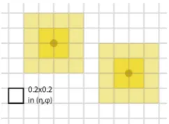
The first rate-reducing step of the ATLAS trigger system is the Level-1 trigger (L1). The L1 jet trigger [3] is based on coarse granularity information from calorimeters. Signals from the calorimeters are aggregated according to detector segments with approximate dimension 0.2×
0.2 in theη-φplane, called jet elements. The dimensions of the jet elements are more irregular in the forward (|η| > 2.5) region. Jet elements are built separately for the electromagnetic and hadronic calorimeters. Regions of interest (RoIs) are defined as windows of 4×4 jet elements (i.e., 0.8×0.8 inη-φ) if they meet two conditions: the summedETfrom the hadronic
calorimeter over their core (2×2 central jet elements) is at a local maximum and the summed
ETover the whole RoI is above a certain predefined threshold (see Figure 1).
Figure 1.Schematic representation of L1 jet elements (grid), RoIs (4×4 yellow squares) and cores (2×2 dark yellow squares). The summedETfrom the hadronic calorimeter within the
cores must be a local maximum for the RoI to be built. The RoI coordinates are those of the centres of the small circles.
2.2 High-level jet trigger
2.2.1 Jet reconstruction
The high-level trigger (HLT) is the final rate-reducing step of the ATLAS trigger system. For the jet HLT, information with full calorimeter granularity is available [4]. Taking the signals from calorimeter cells as input, a three-dimensional topological clustering algorithm is run. Jets are reconstructed with the anti-ktalgorithm using the previously built topological clusters
in 2017 (2018, through 10 September 2018) [2]. This makes triggering on every event with jets not feasible. The same is true for the missing transverse energy (Emiss
T ) computed from
the hadronic component of the event. This is because the pT balance condition is not met
exactly, due to limited resolution in the hadronic calorimeters. If the vector pT imbalances
from several pile-up interactions happen to sum constructively or thepTof a jet is incorrectly
measured, this may result in considerable reconstructedEmiss
T in the event.
The main challenge for the jet andEmiss
T trigger signatures is then to reconstruct features as
closely to the offline reconstruction as possible, using only the limited information available
in the trigger. This should be achieved while ensuring rates do not increase faster than linearly as a function of pile-up.
2 Jet trigger
2.1 Level-1 jet trigger
The first rate-reducing step of the ATLAS trigger system is the Level-1 trigger (L1). The L1 jet trigger [3] is based on coarse granularity information from calorimeters. Signals from the calorimeters are aggregated according to detector segments with approximate dimension 0.2×
0.2 in theη-φplane, called jet elements. The dimensions of the jet elements are more irregular in the forward (|η| > 2.5) region. Jet elements are built separately for the electromagnetic and hadronic calorimeters. Regions of interest (RoIs) are defined as windows of 4×4 jet elements (i.e., 0.8×0.8 inη-φ) if they meet two conditions: the summedETfrom the hadronic
calorimeter over their core (2×2 central jet elements) is at a local maximum and the summed
ETover the whole RoI is above a certain predefined threshold (see Figure 1).
Figure 1.Schematic representation of L1 jet elements (grid), RoIs (4×4 yellow squares) and cores (2×2 dark yellow squares). The summedETfrom the hadronic calorimeter within the
cores must be a local maximum for the RoI to be built. The RoI coordinates are those of the centres of the small circles.
2.2 High-level jet trigger
2.2.1 Jet reconstruction
The high-level trigger (HLT) is the final rate-reducing step of the ATLAS trigger system. For the jet HLT, information with full calorimeter granularity is available [4]. Taking the signals from calorimeter cells as input, a three-dimensional topological clustering algorithm is run. Jets are reconstructed with the anti-ktalgorithm using the previously built topological clusters
as input. For small-Rjets, a parameterR=0.4 is used, while large-Rjets haveR=1.0. The clusters may or may not be weighted prior to jet reconstruction, with weights which depend on their longitudinal depth and energy density. The default procedure is to not apply these weights when reconstructing small-Rjets and to apply them when reconstructing large-Rjets.
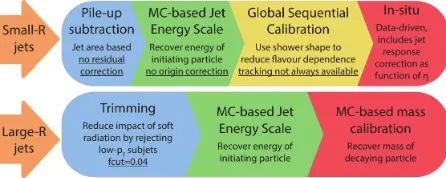
2.2.2 Jet calibration
A calibration sequence is applied to the reconstructed jets as an attempt to recover the ex-pected properties of a corresponding particle-level jet. This is done in a manner as close as possible to the offline jet calibration, within the information constraints of the trigger.
The first step of the calibration of small-Rjets in ATLAS [5], which is the origin cor-rection, depends on vertex reconstruction. This step is not performed in the trigger because tracks are in general not available. The first calibration step applied in the trigger is the jet area based pile-up subtraction, in which the contribution from the median pT density in the
event is removed from jets, proportionally to their area. Residual pile-up corrections depend in part on the number of primary vertices, which again requires tracks, and are thus not ap-plied in the trigger. The following step is the jet energy scale calibration, which corrects the jet energy andηto those expected of a corresponding particle-level jet. Then, the global sequential calibration (GSC) is applied. The offline GSC combines calorimeter, tracking and
muon-segment variables to account for the different detector responses to quark- or
gluon-initiated jets. In the trigger, a reduced version is used, relying on calorimeter information only by default and, in some cases, also using track information. The final step is thein situ
calibration, applied only to data, in which remaining differences between data and MC are
covered.
For large-Rjets [6], the first calibration step is jet grooming, using the trimming algorithm from [7], to reduce dependence on pile-up and the underlying event. This method removes small-Rsubjets of the large-Rjet if they contribute with a fraction smaller thanfto the
large-Rjet pT. The parameter f is set to 5% in the offline calibration and to 4% in the trigger.
This looser threshold in the trigger prevents a trigger inefficiency that was observed if the
same threshold was used as in the offline. Next, an MC-based correction is applied to the
groomed jets. Besides correcting the energy andηof the jets, as happened in small-Rjets, it also corrects their mass. Currently, thein situstep is not applied to large-Rjets [6].
The default trigger jet calibration sequences for small-Rand large-Rjets are summarized in Figure 2, with the main differences with respect to offline highlighted.
Figure 2. Default calibration steps applied to small-R and large-R trigger jets. The main differences with respect to offline are underlined.
3
E
missT
trigger
The L1Emiss
T trigger [8] is based on trigger towers, which are projective calorimeter segments
with approximate dimensions 0.1×0.1 inη-φ(larger and less regular in the forward region). The energy of the trigger towers is calibrated at the electromagnetic energy scale: it correctly reconstructs the energy deposited by particles in an electromagnetic shower but underesti-mates the energy deposited by hadrons. TheEmiss
T is estimated through a vectorial sum of the
Several algorithms have been used for Emiss
T computation at the HLT [4]. The
recom-mended ones during the Run 2 of the LHC have been the jet-based algorithm (mht) and the pile-up fit algorithm (pufit). Themht algorithm computes the Emiss
T as the negative of the
vectorial sum of the pTof small-Rjets, calibrated up to the MC-based jet energy scale step.
The pufitalgorithm uses 112 trigger towers of approximate dimension 0.7×0.8 as input. TheETof each tower is obtained from a sum ofETof topological clusters within the tower.
Then, high-ETtowers are separated from low-ETtowers, with the threshold being determined
on an event-by-event basis, from the mean and variance of towerET. If there is at least one
high-ETtower, a fit is performed to estimate the pile-up contribution to the high-ETtowers. It
uses the low-ETtowers as input and, taking resolution into account, imposes a pile-up energy
density uniform inφand smooth inη, with a null contribution to the totalEmiss
T . TheEmissT is
measured from the high-ETtowers, after subtracting the fitted pile-up contribution.
4 Developments for 2017 and 2018
4.1 L1 jet cone algorithm
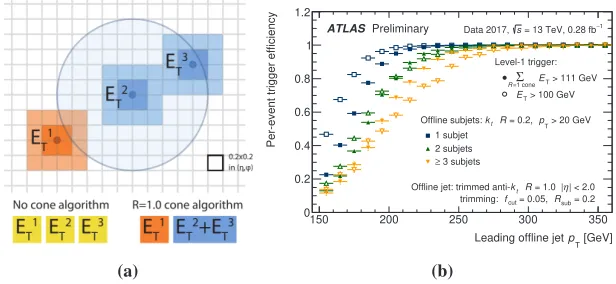
The usual jet RoI definition with anη-φdimension 0.8×0.8 is not adequate to trigger on the large-R(for exampleR = 1.0) jets that are relevant to physics analyses. These jets usually result from the decay of heavy particles and exhibit substructure. If the subjets within the large-Rjet are not close enough, theETwithin the defined RoI(s) can be significantly smaller
than that of the large-Rjet. An additional algorithm was introduced for 2017 data taking to address this inefficiency [9]. It is implemented in the ATLAS Level-1 topological trigger
processor (L1Topo) [10], a system capable of combining information from individual objects and processing it into event-level information. For each RoI, this algorithm searches for other RoIs within 1.0 in∆R(∆R= (∆η)2+(∆φ)2) separation from the original one and sums the
(a)
[GeV] T
p Leading offline jet
150 200 250 300 350
Per-event trigger efficiency
0 0.2 0.4 0.6 0.8 1 1.2
1 subjet 2 subjets
3 subjets
≥
Level-1 trigger: > 111 GeV
T E =1 cone
RΣ
> 100 GeV
T E
Preliminary
ATLAS −1
= 13 TeV, 0.28 fb
s
Data 2017,
> 20 GeV
T p
= 0.2,
R
t
k
Offline subjets:
| < 2.0
η
= 1.0 |
R
t
k
Offline jet: trimmed
= 0.2
sub R
= 0.05,
cut f
trimming:
(b)
Figure 3.(a) L1 jet cone algorithm withR=1.0. The RoIs 2 and 3 may come from the decay of a heavy boson to quarks, for example. They would be clustered together by a large-Rjet algorithm into a high-pTjet, but in L1 trigger they give rise to two lower-ETRoIs. The cone
algorithm adds theirET, resulting in a totalET closer to the large-RjetpT. (b) Efficiency of
the L1 trigger, both with and without the cone algorithm, as a function of the offline leading
large-Rjet pT [11]. The ET threshold with the cone algorithm is adjusted to 111 GeV to
Several algorithms have been used for Emiss
T computation at the HLT [4]. The
recom-mended ones during the Run 2 of the LHC have been the jet-based algorithm (mht) and the pile-up fit algorithm (pufit). The mht algorithm computes theEmiss
T as the negative of the
vectorial sum of the pTof small-Rjets, calibrated up to the MC-based jet energy scale step.
The pufitalgorithm uses 112 trigger towers of approximate dimension 0.7 ×0.8 as input. TheET of each tower is obtained from a sum ofETof topological clusters within the tower.
Then, high-ETtowers are separated from low-ETtowers, with the threshold being determined
on an event-by-event basis, from the mean and variance of towerET. If there is at least one
high-ETtower, a fit is performed to estimate the pile-up contribution to the high-ETtowers. It
uses the low-ETtowers as input and, taking resolution into account, imposes a pile-up energy
density uniform inφand smooth inη, with a null contribution to the totalEmiss
T . TheEmissT is
measured from the high-ETtowers, after subtracting the fitted pile-up contribution.
4 Developments for 2017 and 2018
4.1 L1 jet cone algorithm
The usual jet RoI definition with anη-φdimension 0.8×0.8 is not adequate to trigger on the large-R(for exampleR =1.0) jets that are relevant to physics analyses. These jets usually result from the decay of heavy particles and exhibit substructure. If the subjets within the large-Rjet are not close enough, theETwithin the defined RoI(s) can be significantly smaller
than that of the large-Rjet. An additional algorithm was introduced for 2017 data taking to address this inefficiency [9]. It is implemented in the ATLAS Level-1 topological trigger
processor (L1Topo) [10], a system capable of combining information from individual objects and processing it into event-level information. For each RoI, this algorithm searches for other RoIs within 1.0 in∆R(∆R= (∆η)2+(∆φ)2) separation from the original one and sums the
(a)
[GeV] T
p Leading offline jet
150 200 250 300 350
Per-event trigger efficiency
0 0.2 0.4 0.6 0.8 1 1.2 1 subjet 2 subjets 3 subjets ≥ Level-1 trigger: > 111 GeV
T E =1 cone
RΣ
> 100 GeV
T E
Preliminary
ATLAS −1
= 13 TeV, 0.28 fb
s
Data 2017,
> 20 GeV
T p = 0.2, R t k Offline subjets:
| < 2.0
η
= 1.0 |
R
t
k
Offline jet: trimmed
= 0.2 sub R = 0.05, cut f trimming: (b)
Figure 3.(a) L1 jet cone algorithm withR=1.0. The RoIs 2 and 3 may come from the decay of a heavy boson to quarks, for example. They would be clustered together by a large-Rjet algorithm into a high-pTjet, but in L1 trigger they give rise to two lower-ETRoIs. The cone
algorithm adds theirET, resulting in a totalETcloser to the large-Rjet pT. (b) Efficiency of
the L1 trigger, both with and without the cone algorithm, as a function of the offline leading
large-Rjet pT [11]. TheET threshold with the cone algorithm is adjusted to 111 GeV to
match the same rate as the 100 GeV threshold without the cone algorithm.
ETof such regions. The trigger selection is then applied based on theseETsums and not on
the RoIET(see Figure 3a). In Figure 3b, efficiency curves are shown for L1 jet triggers, both
with and without the cone algorithm. TheET threshold with the cone algorithm is adjusted
to 111 GeV to match the same rate as the 100 GeV threshold without the cone algorithm. For jets with multiple subjets, a desireable sharpening of the turn-on curve is visible, while for jets with a single subjet, only a shift of the turn-on point to a higherpTvalue is visible.
4.2 Improved jet calibration
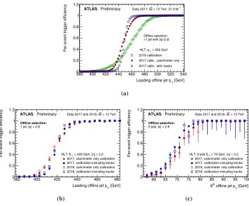
In HLT small-R jet calibration, the GSC andin situ steps were added for 2017 data tak-ing [9]. This brtak-ings the trigger jets much closer to offline jets, which is evident in Figure 4a.
Efficiencies of an unprescaled HLT small-Rsingle jet trigger are compared, for the 2016
cal-ibration, the 2017 calibration with calorimeter-only GSC (default), and the 2017 calibration with the track-dependent GSC (only available for some thresholds andb-jet triggers). The
380 400 420 440 460 480 500 520 540 [GeV] T
p Leading offline jet 0 0.2 0.4 0.6 0.8 1 1.2
Per-event trigger efficiency HLT,pT > 450 GeV 2016 calibration 2017 calib., calorimeter only 2017 calib., with tracks
ATLAS Preliminary Data 2017, s = 13 TeV, 21.9 fb−1
|<2.8 η 1 jet with | ≥ Offline selection:
(a)
380 400 420 440 460 480 [GeV] T
p Leading offline jet 0 0.2 0.4 0.6 0.8 1 1.2
Per-event trigger efficiency HLT:ET > 420 GeV, |η| < 3.2 2017, calorimeter only calibration 2017, calibration including tracks 2018, calorimeter only calibration 2018, calibration including tracks
ATLAS Preliminary Data 2017 and 2018, s = 13 TeV
| < 2.8 η 1 jet, | Offline selection:
(b)
60 65 70 75 80 85 90 95 100 [GeV] T p offline jet th 6 0 0.2 0.4 0.6 0.8 1 1.2
Per-event trigger efficiency HLT: 6 jets ET > 70 GeV, |η| < 3.2 2017, calorimeter only calibration 2017, calibration including tracks 2018, calorimeter only calibration 2018, calibration including tracks
ATLAS Preliminary Data 2017 and 2018, s = 13 TeV
| < 2.8 η 6 jets, | Offline selection:
(c)
Figure 4. (a) Efficiencies of an unprescaled small-R single jet trigger as a function of the
leading offline jet pT, for the 2016 calibration, the 2017 calibration without tracks (default),
and the 2017 calibration with tracks [11]. (b) Efficiencies of an unprescaled small-R
single-jet trigger as a function of the offline leading jet pT, comparing 2017 and 2018 data, with
or without track-based corrections included in GSC [11]. (c) Efficiencies of an unprescaled
small-R six-jet trigger as a function of the offline 6th leading jet pT, comparing 2017 and
full efficiency point is reached for significantly lower offlinepTin 2017 with respect to 2016.
Figures 4b and 4c show efficiency curves comparing the calorimeter-only GSC to the full
GSC in 2017 and 2018 data separately: in Figure 4b for a single jet trigger and in Figure 4c for a six-jet trigger. The curves are similar between the two years, and there is a visibly sharper turn-on when track-based information is included in the GSC.
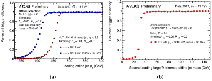
4.3 Mass cut in large-Rtrimmed jets
For large-Rjets, the trimming procedure was also introduced for 2017 data taking, replacing
the previously used area based pile-up subtraction. Large-Rjets are usually regarded in
anal-yses as candidates for boosted hadronically decaying heavy (m mW) particles. Applying
a mass cut to large-Rjets at the trigger level rejects most of the multijet background, while
keeping the signal-like jets. Triggers with such a cut were added as a complement to the
AT-LAS jet trigger menu for 2017 data taking [9]. In Figure 5a, the efficiency of large-Rtrimmed
jet triggers is shown, with and without a mass cut at 35 GeV. The 35 GeV mass cut allows
for a 40 GeV decrease of theET threshold while meeting the trigger menu rate limitations.
Figure 5b shows the efficiency of a large-Rdijet trigger with a 30 GeV mass cut, as a function
of the mass of the second leading offline large-Rjet. Full efficiency is reached for masses
close to 50 GeV.
350 400 450 500 550 600 [GeV] T
p Leading offline jet 0
0.2 0.4 0.6 0.8 1 1.2
Per-event trigger efficiency Trimming: fcut=0.04, Rsub=0.2 > 460 GeV
T
E
> 420 GeV, mass > 35 GeV
T
E
ATLAS Preliminary Data 2017, s = 13 TeV
| < 2.2 η =1.0, | R
Offline selection:
=0.2
sub
R =0.05,
cut
f Trimming:
mass > 50 GeV Blue squares only:
| < 3.2 η =1.0 trimmed jet, | R
HLT:
(a)
trimmed offline jet mass [GeV] R
Second leading
large-0 20 40 60 80 100 120 140
Per-event trigger efficiency
0 0.2 0.4 0.6 0.8 1 1.2
Preliminary
ATLAS Data 2017, s = 13 TeV
Offline selection:
| < 2 η > 400 GeV, |
T
p 2 jets with ≥
= 1.0 R
t
k
= 0.2
sub
R = 0.05,
cut
f trimming:
> 330 GeV, mass > 30 GeV
T
p HLT: 2 jets
(b)
Figure 5. (a) Efficiency of large-Rtrimmed jet triggers, with and without a mass cut at 35
GeV, as a function of the offline leading large-Rtrimmed jet pT [11]. (b) Efficiency of a
large-Rdijet trigger with a 30 GeV mass cut as a function of the mass of the second leading
offline large-Rjet [11].
4.4 pufit algorithm inEmiss T
The use of thepufitalgorithm in theEmiss
T trigger became the primary recommended option in
2017 [9]. In Figure 6a, the efficiency of L1,mhtandpufit ETmisstriggers is compared. Events
shown passed aW →µνselection. Muons are treated as invisible objects for the represented
offlineETmiss, since the same is true for the triggers concerned. The superior performance of
pufitis visible by the steeper turn-on. In Figure 6b, the total trigger cross-section is shown
for anmht Emiss
T trigger and apufittrigger, as a function of the mean number of interactions
per bunch-crossingµ. The rate increase is slower forpufit, which makes it more stable with
full efficiency point is reached for significantly lower offlinepTin 2017 with respect to 2016.
Figures 4b and 4c show efficiency curves comparing the calorimeter-only GSC to the full
GSC in 2017 and 2018 data separately: in Figure 4b for a single jet trigger and in Figure 4c for a six-jet trigger. The curves are similar between the two years, and there is a visibly sharper turn-on when track-based information is included in the GSC.
4.3 Mass cut in large-Rtrimmed jets
For large-Rjets, the trimming procedure was also introduced for 2017 data taking, replacing
the previously used area based pile-up subtraction. Large-Rjets are usually regarded in
anal-yses as candidates for boosted hadronically decaying heavy (m mW) particles. Applying
a mass cut to large-Rjets at the trigger level rejects most of the multijet background, while
keeping the signal-like jets. Triggers with such a cut were added as a complement to the
AT-LAS jet trigger menu for 2017 data taking [9]. In Figure 5a, the efficiency of large-Rtrimmed
jet triggers is shown, with and without a mass cut at 35 GeV. The 35 GeV mass cut allows
for a 40 GeV decrease of theET threshold while meeting the trigger menu rate limitations.
Figure 5b shows the efficiency of a large-Rdijet trigger with a 30 GeV mass cut, as a function
of the mass of the second leading offline large-Rjet. Full efficiency is reached for masses
close to 50 GeV.
350 400 450 500 550 600 [GeV] T
p Leading offline jet 0 0.2 0.4 0.6 0.8 1 1.2
Per-event trigger efficiency Trimming: fcut=0.04, Rsub=0.2 > 460 GeV
T
E
> 420 GeV, mass > 35 GeV
T
E
ATLAS Preliminary Data 2017, s = 13 TeV
| < 2.2 η =1.0, | R Offline selection: =0.2 sub R =0.05, cut f Trimming:
mass > 50 GeV Blue squares only:
| < 3.2 η =1.0 trimmed jet, | R
HLT:
(a)
trimmed offline jet mass [GeV] R
Second leading
large-0 20 40 60 80 100 120 140
Per-event trigger efficiency
0 0.2 0.4 0.6 0.8 1 1.2 Preliminary
ATLAS Data 2017, s = 13 TeV
Offline selection:
| < 2 η > 400 GeV, |
T
p 2 jets with ≥ = 1.0 R t k = 0.2 sub R = 0.05, cut f trimming:
> 330 GeV, mass > 30 GeV
T
p HLT: 2 jets
(b)
Figure 5. (a) Efficiency of large-Rtrimmed jet triggers, with and without a mass cut at 35
GeV, as a function of the offline leading large-Rtrimmed jet pT [11]. (b) Efficiency of a
large-Rdijet trigger with a 30 GeV mass cut as a function of the mass of the second leading
offline large-Rjet [11].
4.4 pufit algorithm inEmiss T
The use of thepufitalgorithm in theEmiss
T trigger became the primary recommended option in
2017 [9]. In Figure 6a, the efficiency of L1,mhtandpufit EmissT triggers is compared. Events
shown passed aW →µνselection. Muons are treated as invisible objects for the represented
offlineETmiss, since the same is true for the triggers concerned. The superior performance of
pufitis visible by the steeper turn-on. In Figure 6b, the total trigger cross-section is shown
for anmht Emiss
T trigger and apufittrigger, as a function of the mean number of interactions
per bunch-crossingµ. The rate increase is slower forpufit, which makes it more stable with
respect to increasing luminosity.
(offline, no muons) [GeV]
miss T
E
0 50 100 150 200 250 300
Efficiency 0 0.2 0.4 0.6 0.8 1 L1_XE50 HLT_xe110_pufit_L1XE50 HLT_xe110_mht_L1XE50 Data 2017 -1
= 13 TeV, 1.3 fb s ν µ → W ATLAS Preliminary (a) > µ < 10 15 20 25 30 35 40 45 50 55
Trigger cross section [nb]
0 10 20 30 40 50 60 ATLAS Trigger Operations HLT_xe110_mht_L1XE50 HLT_xe110_pufit_L1XE50
= 13 TeV s Data 2016 / 2017,
(b)
Figure 6. (a) Efficiency of L1, mht and pufit EmissT triggers as a function of the offline Emiss
T [12]. (b) Total trigger cross-section as a function ofµfor mhtandpufit EmissT
trig-gers with a 110 GeV threshold [12].
5 Conclusions
Efficient triggering on hadronic signatures (jets and hadronicETmiss) is crucial for the ATLAS
physics programme. The increasing luminosity during Run 2 of the LHC made this task particularly challenging. For the data taking periods of 2017 and 2018, the ATLAS jet and Emiss
T triggers implemented new strategies to face this challenge. These included improving
jet calibration, exploiting the substructure of large-R jets and using a much more pile-up
insensitiveEmiss
T reconstruction algorithm.
6 Acknowledgements
E. G. is funded by Fundação para a Ciência e Tecnologia, through grant PD/BD/128231/2016.
References
[1] ATLAS Collaboration, JINST3, S08003 (2008)
[2] ATLAS Collaboration,
https://twiki.cern.ch/twiki/bin/view/AtlasPublic/LuminosityPublicResultsRun2
[3] ATLAS Collaboration, Eur. Phys. J. C76, no.10, 526 (2016)
[4] ATLAS Collaboration, Eur. Phys. J. C77, no.5, 317 (2017)
[5] ATLAS Collaboration, Phys. Rev. D96, no.7, 072002 (2017)
[6] ATLAS Collaboration, Eur. Phys. J. C79, no.2, 135 (2019)
[7] D. Krohn, J. Thaler and L. T. Wang, JHEP1002, 084 (2010)
[8] ATLAS Collaboration, ATL-DAQ-PUB-2018-001 [9] ATLAS Collaboration, ATL-DAQ-PUB-2018-002 [10] E. Simioni, arXiv:1406.4316 [physics.ins-det] [11] ATLAS Collaboration,
https://twiki.cern.ch/twiki/bin/view/AtlasPublic/JetTriggerPublicResults
[12] ATLAS Collaboration,