Western University Western University
Scholarship@Western
Scholarship@Western
Electronic Thesis and Dissertation Repository
4-16-2015 12:00 AM
Online Nonparametric Estimation of Stochastic Differential
Online Nonparametric Estimation of Stochastic Differential
Equations
Equations
Xin Wang
The University of Western Ontario
Supervisor Duncan Murdoch
The University of Western Ontario Joint Supervisor Matt Davison
The University of Western Ontario
Graduate Program in Statistics and Actuarial Sciences
A thesis submitted in partial fulfillment of the requirements for the degree in Doctor of Philosophy
© Xin Wang 2015
Follow this and additional works at: https://ir.lib.uwo.ca/etd
Part of the Statistical Theory Commons
Recommended Citation Recommended Citation
Wang, Xin, "Online Nonparametric Estimation of Stochastic Differential Equations" (2015). Electronic Thesis and Dissertation Repository. 2755.
https://ir.lib.uwo.ca/etd/2755
This Dissertation/Thesis is brought to you for free and open access by Scholarship@Western. It has been accepted for inclusion in Electronic Thesis and Dissertation Repository by an authorized administrator of
(Thesis format: Monograph)
by
Xin Wang
Graduate Program in Statistics and Actuarial Science
A thesis submitted in partial fulfillment
of the requirements for the degree of
Doctor of Philosophy
The School of Graduate and Postdoctoral Studies
The University of Western Ontario
London, Ontario, Canada
c
Abstract
The advent of the big data era presents new challenges and opportunities for those managing portfolios, both of assets and of risk exposures, for the financial industry. How to cope with the volume of data to quickly extract actionable information is becoming more crucial than ever before. This information can be used, for example, in pricing various financial products or in calculating risk exposures to meet (ever changing) regulatory requirements.
Stochastic differential equations are often used to model the risk factors in finance. Giv-en the presumption of a functional form for the coefficients of these equations, the required parameters can be calibrated using a large body of statistical techniques which have been de-veloped over the past decades. However, the price to pay for this convenience is the problems that occur if an incorrect functional form is used. To avoid this problem of misspecification, nonparametric regression has recently become important in finance. In order to adequately es-timate local structures, large sample sizes are always required and so nonparametric regression is computationally intensive.
This thesis finds new ways to decrease the computational cost of non-parametric meth-ods for estimating stochastic differential equations. Motivated by stochastic approximations, we propose online nonparametric methods to estimate the drift and diffusion terms of typical financial stochastic differential equations. Both stationary and non-stationary processes are considered and this thesis provides asymptotic properties of the estimators. For the stationary case, quadratic convergence, strong consistency, and asymptotic normality of the estimators are established; for the non-stationary case, weak consistency of the estimators is proved.
In addition to numerical examples, we also apply our methods to market risk management. We work from up to date examples based on the most recent Basel Committee documents for a wide range of risk factors from equity, foreign exchange, interest rates, and commodity prices. The advantages and disadvantages of applying our new statistical techniques to these risk management problems are also discussed.
Keywords: online nonparametric estimation, stochastic differential equations, financial
modeling
When writing this part, I come to realize that my student life will become memories of the past. Recalling the last two years, from a novice in statistics and finance to writing this thesis, I know how I benefited from the guidance and support of many people.
I greatly appreciate my supervisors, Dr. Murdoch and Dr. Davison, for their valuable guidance, patience and enthusiasm during the years of my doctoral research. Dr. Murdoch’s insight and knowledge in statistics broadened my horizons and deepened my understanding in statistics, while Dr. Davison led me into the realm of finance and gave me an intuition beneath the complicated concepts and techniques. They are my most valuable assets.
I would also like to thank my committee members, Dr. Reg Kulperger, Dr. Lars Stentoft, Dr. Hubert Pun and Dr. Adam Kolkiewicz, for their constructive feedback. Many thanks are given to my colleagues in TD Bank and office mates in the university for their kindness and support.
Also, I am very grateful to my parents for their endless love, encouragement, support and patience throughout my life.
Finally, my deep love goes to my wife Sulin Cheng, for her sacrifice and support, always by my side whenever in my busy or dark times, all that keep me going.
Contents
Abstract ii
Acknowledgements iii
List of Figures vi
List of Tables ix
1 Introduction 1
1.1 Background and Motivation . . . 1
1.2 Ideas and Contributions . . . 2
1.3 Outline of This Thesis . . . 4
2 Kernel Methods in Risk Management 5 2.1 Market Risk Management . . . 5
2.1.1 Risk Measures . . . 5
2.1.2 Approaches . . . 7
2.2 Kernel Methods . . . 12
2.2.1 Kernel Density Estimators . . . 13
2.2.2 Kernel Regression Estimators . . . 13
2.2.3 Choice of Bandwidth and Kernel Function . . . 16
2.3 Example . . . 20
3 Literature Review 22 3.1 Time-Homogeneous Diffusion Models . . . 22
3.2 Second-Order Diffusion Models . . . 27
3.3 Time-Inhomogeneous Diffusion Models . . . 28
3.4 Remark . . . 30
4 Asymptotic Theory of Online Estimators for SDE 31 4.1 Introduction . . . 31
4.2 Method . . . 32
4.3 Theoretical Analysis . . . 33
4.3.1 Assumptions and Preliminary Lemmas . . . 33
4.3.2 Quadratic Convergence . . . 35
4.3.3 Strong Consistency . . . 43
4.3.4 Asymptotic Normality . . . 47
4.4 Concluding Remark . . . 59
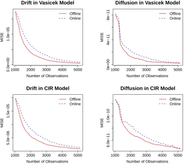
5.1.1 Comparison with offline estimators . . . 62
5.1.2 Sensitivity to parameters . . . 67
5.2 Case Study: US 3-Month Treasury Bill Rates . . . 71
5.2.1 Estimation Results . . . 74
5.2.2 Application in Risk Management . . . 79
5.3 Concluding Remark . . . 85
6 Online Kernel Estimators for Second-Order Diffusion Models 88 6.1 Method . . . 88
6.2 Theoretical Analysis . . . 89
6.2.1 Assumptions and a Preliminary Lemma . . . 89
6.2.2 Weak Consistency . . . 90
6.3 Examples . . . 95
6.3.1 Numerical Simulation . . . 95
6.3.2 Real Application . . . 97
6.4 Concluding Remark . . . 105
7 Conclusion and Future Work 106 7.1 Contributions . . . 106
7.2 Future Work . . . 107
Bibliography 109
Appendix A Stochastic differential Equations 118
Appendix B Stochastic Approximation 124
Appendix C Mixing Processes 128
Curriculum Vitae 132
List of Figures
2.1 S&P/TSX Composite Index during the period from Jun 29, 1979 to Nov 2, 2014 (top) and Canadian 3-Month Treasury Bill Rate during the period from Nov 2, 2004 to Oct 31, 2014 (bottom). . . 6 2.2 Demonstration of VaR, where the percentage of the shaded area is 1−α. . . 6 2.3 Demonstration of historical simulation, whereτ = 1, T = 250 and N = 251.
So in this case, the 99% VaR is△x(3) and 97.5% ES is the average of△x(1) to
△x(7). . . 8
2.4 Historical simulation for S&P/TSX Composite Index where daily shocks are used for demonstration and 99% VaR and 97.5% ES are calculated to compare with PnL. The darkest bar represents the red zone, the lightest bar represents the yellow zone and the rest represents the green zone. . . 9 2.5 The Monte Carlo method for S&P/TSX Composite Index where 99% VaR and
97.5% ES are calculated to compare with PnL. The darkest bar represents the red zone, the lightest bar represents the yellow zone and the rest represents the green zone. . . 11 2.6 Boundary effect for the Nadaraya-Watson estimator and the local linear
estima-tor, where the data are generated byy = −(x−0.5)2+0.05εwithε∼ N(0,1).
The solid line is the true curve y = −(x−0.5)2, and the dotted line gives the fitted values. . . 16 2.7 Four Nadaraya-Watson estimators for Canadian male wage data on 1971, where
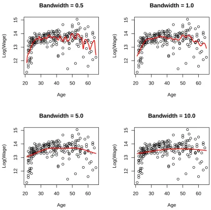
the bandwidth arehn= 0.5,hn= 1.0,hn= 5.0 andhn =10.0. . . 17
2.8 The leave-one-out CV is performed on the same Canadian male wage data seen in Figure 2.7 (left) andy= −(x−0.5)2(right). The optimal bandwidth is
hoptn =1 for the left andh
opt
n =0.01 for the right. . . 18
2.9 Historical simulation for S&P/TSX Composite Index where daily shocks are used for demonstration and 99% VaR and 97.5% ES are calculated to compare with PnL. All trading days are in green zone. . . 20 5.1 The sample path of (5.1) and (5.2) with the same random seed where△=1/260
andT = 20. . . 62 5.2 Demonstration of MISE for sequential observations, parameters as in Table 5.1. 63 5.3 Fitting values by offline and online estimators which are averaged on 1000
replications, and the 95% confidence band of the online estimators, parameters as in Table 5.1. . . 64 5.4 MISE for both offline and online estimators when △ = 1/12 and 1/52 given
n=1000 andm=0.2n. . . 65 5.5 MISE for both offline and online estimators when T = 10 and 50 given △ =
1/260 andm= 0.2n. . . 65
band. . . 68
5.7 Sensitivity toT = 10,15 and 20 where△=1/260 andm=0.2n. The solid line represents the true value and the shadow area is the 95% confidence band. . . . 69
5.8 Sensitivity to m = 0.1n,0.3nand 0.5ngiven △ = 1/260 andn = 5200, where the solid line represents the true value and the shadow area is the 95% confi-dence band. . . 70
5.9 The daily US 3-month treasury bill rates from May 8, 1978 to November 14, 2014. . . 71
5.10 The absolute shocks of the daily US 3-month treasury bill rates. . . 72
5.11 Histogram and QQ-plot of the US 3-month treasury bill rates between May 8, 1978 and November 14, 2014. . . 72
5.12 Nonparametric marginal density of the data, where the solid line represents true values and the shadow area is the 95% confidence band. . . 73
5.13 Comparison between nonparametric marginal density function and those of the Vasicek and CIR model. . . 75
5.14 Estimation of the drift and diffusion by the calibrated Vasicek and CIR model, and the online method with different bandwidths hi = σˆi ×i−0.2 (the top) and hi =σˆi×i−0.02(the bottom). . . 76
5.15 Estimation of the drift and diffusion as well as 90% pointwise confidence band by the online method for the bandwidths hi = σˆi × i−0.2 (the top) and hi = ˆ σi×i−0.02(the bottom). . . 77
5.16 Comparison of the drift and diffusion specification by the offline and online methods for the bandwidths hi = σˆi ×i−0.2 (the top) and hi = σˆi × i−0.02 (the bottom). . . 78
5.17 Calculation of -VaR by historical simulation, Monte Carlo method by the Va-sicek and CIR model, and online method, where the dashed line is shocks and the solid line is -VaR. . . 81
5.18 Calculation of -ES by historical simulation, Monte Carlo method by the Va-sicek and CIR model, and online method, where the dashed line is shocks and the solid line is -ES. . . 82
5.19 95% Confidence band for daily 99% VaR and 97.5% ES by historical simula-tion and the online method. . . 85
5.20 20-day 99% VaR and 97.5% ES by historical simulation. . . 86
6.1 The sample path of (6.7) as well as the integrated process . . . 95
6.2 MISE behaviors of (6.4) and (6.6) for sequential observations . . . 96
6.3 The 95% confidence band of the estimators (6.4) and (6.6). The solid line is the true value. . . 96
6.4 The time series of the stock index GSPTSE, DJI, IXIC and SSE from Jan 2, 1991 to Jan 16, 2015. . . 97
6.5 The proxy of the stock index GSPTSE, DJI, IXIC and SSE (daily data from Jan 2, 1991 to Jan 16, 2015). . . 98
6.6 Online estimation of the drift and diffusion in the latent process {Xi}˜ for the stock index GSPTSE, DJI, IXIC and SSE. . . 100
6.7 The FX rate of CAD/CNY, CAD/USD, CAD/GBP and CAD/EUR from Jan 31, 2010 to Jan 16, 2015. . . 101 6.8 The proxy of CAD/CNY, CAD/USD, CAD/GBP and CAD/EUR. . . 102 6.9 Online estimation of the drift and diffusion in the latent process{Xi}˜ for the FX
rate CAD/CNY, CAD/USD, CAD/GBP and CAD/EUR. . . 103 6.10 The time series of the crude oil prices and gold prices as well as their proxies. . 104 6.11 Online estimation of the drift and diffusion in the latent process {Xi}˜ for the
crude oil prices and gold prices. . . 105 A.1 Trajectories of GBM and Brownian motion, where GBM is dXt = 0.2Xtdt +
0.375XtdWt. . . 120 A.2 Stock prices of RBC, TD Bank, BMO, Scotiabank and CIBC where data are
from Yahoo! Finance and the time interval is from Jan 3, 2007 to Nov 6, 2014. . 123 B.1 Demonstration of the Robbins-Monro algorithm. . . 125
5.1 Common parameters in simulation. . . 63
5.2 Running time for△ = 1/12,1/52 and 1/260 where n = 1000 and m = 0.2n. That is, the time period T = n△ = 1000/12,1000/52 and 1000/260 for each case. . . 66
5.3 Running time forT =10,20 and 30 given△=1/260 andm=0.2n. . . 66
5.4 Running time form=0.1n,0.3n,0.5nand 0.7nwhere△ =1/260 andn=5200. 67 5.5 Summary statistics of US 3-month treasury bill rates between May 8, 1978 and November 14, 2014. . . 72
5.6 Hypothesis tests of the data for the stationarity, independence and normality. . . 73
5.7 Calibration of parameters in the Vasicek and CIR model. . . 75
5.8 Comparison of VaR and ES . . . 80
6.1 Augmented Dickey-Fuller stationarity test of stock indices GSPTSE, DJI, IXIC and SSE as well as their proxies. . . 99
6.2 The calibrated parameters if GBM is assumed to model the stock index. . . 99
6.3 The convergent bandwidth in online estimators of the drift and diffusion. . . 99
6.4 The calibrated parameters if GBM is assumed to model the FX rate. . . 102
A.1 Estimation of the drift and diffusion for the stock prices of RBC, TD Bank, BMO, Scotiabank and CIBC from Jan 3, 2007 to Nov 6, 2014. . . 123
Chapter 1
Introduction
This thesis proposes online nonparametric estimators for stochastic differential equations, espe-cially for time-homogeneous diffusion models. For the stationary case, we establish quadratic convergence, strong consistency and asymptotic normality of our estimators. Numerical exam-ples and a case study are used to validate effectiveness and efficiency of our methods. For the non-stationary case, a class of second-order stochastic differential equations is considered and online estimators are proposed and studied.
In this chapter, we first present background materials and some motivation for this thesis. Then the ideas and our contributions are discussed. Finally the organization of this thesis is outlined.
1.1
Background and Motivation
Stochastic differential equations (SDEs) are an essential tool to describe the randomness of a dynamic system. For example, physicists use this tool to model the time evolution of particles due to thermal fluctuations (Sobczyk, 2001) and ecologists study two interacting populations such as predator and prey by SDEs (Allen, 2007). In the financial system, many different SDEs have been developed to model a particular financial product or class of products, e.g. geometric Brownian motion (GBM) by Osborne (1959) for modeling stock prices or stock indices, and for modeling interest rates the Vasicek model (Vasicek, 1977), the CIR model (Cox et al., 1985) and the CKLS model (Chan et al., 1992). Financial institutions make use of SDEs to price their derivatives or measure the risks of their portfolios. For example, when pricing financial products, one needs to specify the form of SDEs driving the appropriate randomness and then estimate the parameters of interest in the equation to generate future scenarios; when measuring risks, one needs to calculate shocks based on these generated scenarios to obtain Value-at-Risk or Expected Shortfall. Therefore, this presumption of functional forms is always considered as a parametric method.
In the last two decades, nonparametric regression has attracted more academic and pro-fessional attention. The reason for this growing attention is that nonparametric regression is distribution-free, i.e. requiring little prior information on the data generation, so misspecifica-tion in the parametric method can be avoided. Now nonparametric regression has become a vital area in statistics (H¨ardle, 1990; Li and Racine, 2006) and it has many successful applica-tions in finance (Campbell et al., 1988; Tsay, 2005). When nonparametric regression is applied in finance, an approach is to study the general SDE
dXt =a(t,Xt)dt+b(t,Xt)dWt (1.1)
wherea(t,Xt) andb2(t,Xt) are the functions of our concern, called the drift and diffusion
coef-ficients respectively1. They represent the expected return and volatility of the underlying
vari-able, and are important factors to price assets, manage risks and choose portfolios. Through discretization of the equation, one can derive nonparametric estimators for the drift and dif-fusion coefficients by kernel methods (Fan and Gijbels, 1996) or smoothing splines (Wahba, 1990), and use these estimators to fulfill the financial purpose.
However, relaxing the assumption on the data generation in nonparametric regression does not come at no cost. In fact, compared to its parametric counterparts, nonparametric regression is computationally intensive. One reason is that each nonparametric estimator is the result of multiple local fits. Modern computers have drastically reduced the running time of the meth-ods making them more practically available than ever before. But nonparametric regression uses the data themselves to tell the story, so larger sample sizes are always required to keep local structures for estimation. This implies that the computational cost is still quite large. In addition, nonparametric estimation methods have lower rate of convergence. This could be a serious impediment in some financial applications, where often time series exhibit non-stationary behavior that prevents us from using longer data sets. Thus we need new ways to lower the computational cost as well as make accurate estimates, which is our motivation of this thesis.
1.2
Ideas and Contributions
If we have the current data items of (x1,y1),(x2,y2), . . . ,(xn,yn) and must estimate the value ofy
atxwherex, xifor 1≤ i≤n, in this case we can use nonparametric regresion (such as kernel
regression) to achieve this task. But at the moment a new observation (xn+1,yn+1) is available,
then in order to obtain the real-time estimate, we have to use nonparametric regression again
1Sometimes b(t,X
t) is called the diffusion (Fan and Zhang, 2003) but some works refer tob2(t,Xt) as the
1.2. Ideas andContributions 3
for alln+1 data items. It is clear that the complexity2of this procedure is at leastO(n). When a great deal of data are available sequentially and real-time estimation is required, it is not hard to imagine that nonparametric regression is not adequate to this job because the computational cost is quite large. This often happens in real cases. Financial institutions need to calculate Value-at-Risk and Expected Shortfall so as to meet the regulator’s capital requirement, but in order to fulfill this task, they calibrate the parameters in the model by combining existing observations and the use of Monte Carlo simulation to generate scenarios. Often large financial institutions have very complicated portfolios. This means that they obtain millions of new observations each business day and so should use all their existing data plus the new data to repeat their calculations. Therefore how to obtain real-time results for a huge quantity of time series data is an important issue in practice.
However note that the previous estimate of the value of interest contains important histori-cal information and can be used to derive the new one, so each time it is not necessary to use all current and all historical data. In this thesis, one of our main contributions is to propose an incremental way of computing nonparametric estimates for SDEs (called online methods3) and apply our methods in finance. In our methods, new data are used to update the previous estimate to yield the new one, hence the complexity of each update isO(1) which is far better thanO(n) whennis large. Our methods can meet real-time demand in financial institutions.
This thesis studies the diffusion process as described in (1.1) and proposes online kernel estimators for the drift and diffusion. Here our main focus is on the diffusion process driven by Brownian motion instead of by other more general L´evy processes because such kind of processes are widely used in practice. We consider the time-homogeneous case, that is, the drift and diffusion do not depend on the timetdirectly
dXt =a(Xt)dt+b(Xt)dWt (1.2)
In this thesis, we study both stationary and non-stationary processes. For example, GBM is a non-stationary time-homogeneous process; the Vasicek model, CIR model and CKLS model are stationary time-homogeneous processes. In addition, we theoretically prove quadratic con-vergence, strong consistency and asymptotic normality of online estimators for the stationary case, and weak consistency for the non-stationary case. By simulation we validate eff ective-ness and efficiency of our methods for both the stationary and non-stationary cases. We also test these new methods in real applications to calculate Value-at-Risk and Expected Shortfall for market risk management.
2In computer science, “big O” and “small o” are widely used notations to measure the computational
com-plexity. Given two sequences{an}and{bn}, thenan=O(bn) means|an| ≤c|bn|wherecis some positive constant,
whereasan=o(bn) meansan/bn →0 asn→ ∞. Thusan =O(1) indicatesanis bounded andan =o(1) implies
an → 0. Additionally in probability theory, given a random variable sequence{Xn}, thenXn =op(1) meansXn
converges to zero in probability, i.e. limn→∞P(|Xn|> ε)=0 for anyε >0.
There are several things to note in this thesis. First, we propose online kernel-type esti-mators because in practice kernel methods are easy to implement. But similar ideas can be used to derive estimators of other types such as smoothing splines. Second, we are concerned with high-frequency data. With the development of modern technology, more data are mea-sured every minute, so called one minute bars, and have become available than ever before. So it is of practical significance to propose online estimators for high-frequency data. Third, we build up estimators on a discrete-time sample of observations. Although the continuous sample path has been considered for many years (Rao, 1999), it is impossible to obtain with digital continuous-time observations in real applications. Thus our estimators are derived from discrete-time observations. Fourth, previous studies on nonparametric estimation of SDEs give offline estimators. To the best of our knowledge online nonparametric estimation has never been applied to SDEs, therefore our work bridges the gap between these areas and supplies feasible estimators for financial practice. Additionally, we give the rate of mean squared errors and asymptotic normality for further inference such as constructing confidence intervals.
1.3
Outline of This Thesis
Chapter 2
Kernel Methods in Risk Management
Since the 2007 financial crisis, the importance of the internal control has become clear not just to risk management but to the entire world. Yet risk management failures continue. For example, JP Morgan suffered large trading losses in 2012 for its ineffectiveness and failure of risk management in controlling trading activities, so-called the “London Whale” case1. A similar case occurred in 2013 at Everbright Securities, a Chinese Brokerage, because of the lack of risk management systems for monitoring trading errors2. On the other hand, there have been many studies of kernel methods in different areas such as finance (Fan and Yao, 2013), economics (Li and Racine, 2006) and meteorology (Xu, 2008), but little attention is paid to their applications for risk management. In this chapter, we first introduce the basic concepts and methods of both market risk management and kernel methods. Then we give an example to illustrate how to apply kernel methods to measure market risk.
2.1
Market Risk Management
As is shown in Figure 2.1, the prices of most financial products (e.g. stocks, bonds and their derivatives) fluctuate all the time. When financial institutions include these products into their portfolios, they have to use approaches to measure the risks of the exposure to these risk factors.
2.1.1
Risk Measures
Value-at-Risk (VaR) is a widely used measure of the market risk of losses on a portfolio. LetX
denote the profit-and-loss (PnL) of a portfolio over a time periodt, then the VaR of the portfolio is defined as follows:
VaRα =sup{−x: Pt(X> x)≤α} (2.1) 1See details inhttp://en.wikipedia.org/wiki/2012_JPMorgan_Chase_trading_loss.
2See details in
http://www.bloomberg.com/news/2013-08-16/everbright-securities-investigates-trading-system-error-1-.html.
1980 1990 2000 2010
2000
10000
S&P/TSX Composite Index
Time
Inde
x
2006 2008 2010 2012 2014
0
2
4
Canadian 3−Month Treasury Bill Yield
Time
Y
ield (P
ercent)
Figure 2.1: S&P/TSX Composite Index during the period from Jun 29, 1979 to Nov 2, 2014 (top) and Canadian 3-Month Treasury Bill Rate during the period from Nov 2, 2004 to Oct 31, 2014 (bottom).
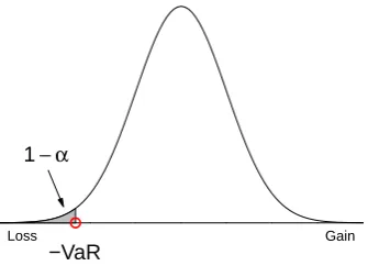
whereα∈(0,1) is a significance level, e.g. taking 99% or 99.9%, see demonstration in Figure 2.2. From the definition, it can be seen that VaR estimation has the prediction of tail losses as its primary goal.
1− α
−VaR
Loss Gain
Figure 2.2: Demonstration of VaR, where the percentage of the shaded area is 1−α.
2.1. MarketRiskManagement 7
and not a coherent risk measure (Schied, 2006). Hence the Basel Committee suggest using the Expected Shortfall (ES) as an alternative. This ES metric is also called the conditional VaR and is given by
ESα =E[−X|X ≤ −VaRα] (2.2) Different from VaR, the above definition of ES is about the expected loss given that the PnL is “bad”. It can be found that ES is more sensitive to the shape of tail events because it provides more information on the tail.
Note that (2.1) and (2.2) are related to the distribution function ofX, which unfortunately is usually unknown to us. In this case, it is often practical to use order statistics of Xto calculate VaR and ES instead. Let X1,X2, . . . ,Xn be nindependently and identically distributed (i.i.d.)
samples ofX, and thek-th order statistic denoted by X(k). Then an empirical way to calculate
VaR and ES (Hull, 2012) is listed as below
VaRα = −X(⌈n(1−α)⌉) (2.3)
ESα = −1
⌈n(1−α)⌉
⌈n∑(1−α)⌉
i=1
X(i) (2.4)
For example, if there aren=100,000 PnL scenarios, then 99.9% VaR is the 100th worst value and 97.5% ES is the average of the first 2,500 values in ordered PnL scenarios.
2.1.2
Approaches
The PnL distribution can be used to calculate VaR and ES according to (2.1) and (2.2). This part introduces two main approaches, historical simulation and the Monte Carlo method, about estimation of the PnL distribution based on a time series of observations. Let {Xt}denote the time series of some risk factor with liquidity horizon τ and time horizon T. For example, the Basel Committee prescribe a liquidity horizon for the interest rate be 20 days and a time horizon be at least one year.
Historical Simulation
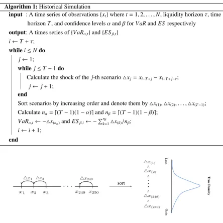
Algorithm 1:Historical Simulation
input : A time series of observations{xt}wheret=1,2, . . . ,N, liquidity horizonτ, time horizonT, and confidence levelsαandβforVaRandES respectively
output: A times series of{VaRα,t}and{ESβ,t}
i← T +τ;
whilei≤N do
j←1;
while j≤ T −1do
Calculate the shock of the j-th scenario△xj = xi−T+j−xi−T+j−τ;
j← j+1;
end
Sort scenarios by increasing order and denote them by△x(1),△x(2), . . . ,△x(T−1);
Calculatenα = ⌈(T −1)(1−α)⌉andnβ =⌈(T −1)(1−β)⌉;
VaRα,i ← −△x(nα)andESβ,i ← −∑
nβ
k=1△x(k)/nβ;
i← i+1;
end
sort
Loss
Gain
T
rue
Density
<
<
<
<
Figure 2.3: Demonstration of historical simulation, whereτ= 1,T = 250 andN = 251. So in this case, the 99% VaR is△x(3)and 97.5% ES is the average of△x(1)to△x(7).
2.1. MarketRiskManagement 9
1980 1990 2000 2010
−500
500
Historical Simulation for S&P/TSX Composite Index
Time
Shock
PnL −VaR0.99
1980 1990 2000 2010
−500
500
Historical Simulation for S&P/TSX Composite Index
Time
Shock
PnL −ES0.975
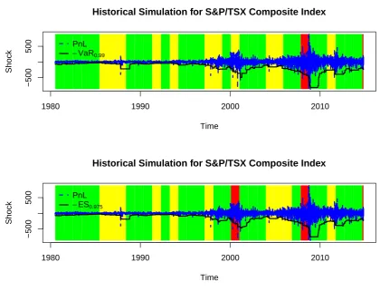
Figure 2.4: Historical simulation for S&P/TSX Composite Index where daily shocks are used for demonstration and 99% VaR and 97.5% ES are calculated to compare with PnL. The darkest bar represents the red zone, the lightest bar represents the yellow zone and the rest represents the green zone.
Despite its simplicity and distribution-free assumption, there are three restrictions of his-torical simulation. First, it uses equal weights for all PnLs. But more recent experience might be more important or, alternatively, experience observed at past times judged to be similar to the present in the business cycle might be deemed more important. Thus weighted historical simulation has been studied (Boudoukh et al., 1998). Second, historical simulation uses the past observations to yield its predictions. This means that the number of scenarios are limited to those actually experienced, a major restriction. Hence multiyear time horizon is often used (Mehta et al., 2012). Third, independent and identical distribution of the shocks is assumed in using historical simulation, but it could be violated for the shocks with overlapped time interval. So a filtered method has been devised for correlated data (Barone-Adesi et al., 1999).
Monte Carlo Method
Therefore, it can provide a comprehensive picture of risks in the tail distribution. In addition, once the model is specified, as many scenarios as one likes can be obtained by the Monte Carlo method.
There is no general procedure for the Monte Carlo method because it is different from case to case. We use a simple example to illustrate its application to calculate VaR and ES, where GBM is used to model S&P/TSX Composite Index. The introduction to SDEs including GBM can be seen in Appendix A. For GBMdXt =µXtdt+σXtdWt, the parameters are estimated by
(A.13), that is,
ˆ
µ= m+△s2/2 and σˆ = √s
△
wherem = n−1∑ni=−01Ri, s2 = (n−1)−1∑ni=−01(Ri−m)2 and Ri = log(Xi+1)−log(Xi) is the
log-return over the time horizon as is considered. Then the procedure of the Monte Carlo method for GBM is listed as below
Algorithm 2:The Monte Carlo method for GBM
input : A time series of observations{xt}wheret=1,2, . . . ,N, discretization step size
△, time horizonT, sample sizen, and confidence levelsαandβforVaRandES
respectively
output: A times series of{VaRα,t}and{ESβ,t}
i← T +1;
whilei≤N do
j←1;
while j≤ T −1do
Calculate the log-returnsrj =log(xi−j)−log(xi−j−1);
j← j+1;
end
Calculatemi = (T −1)−1
∑T−1
k=1 rk ands2i =(T −2)−1
∑T−1
k=1(rk−mi)2;
Base on (A.13) to calculate ˆµi and ˆσi;
Based on (A.9), generate samples ˆxi,1,xˆi,2, . . . ,xˆi,n;
Calculate the PnL△xj = xˆi,j−xi−1;
Calculatenα = ⌈(T −1)(1−α)⌉andnβ =⌈(T −1)(1−β)⌉;
VaRα,i ← −△x(nα)andESβ,i ← −
∑nβ
k=1△x(k)/nβ;
i← i+1;
end
2.1. MarketRiskManagement 11
1980 1990 2000 2010
−500
500
Monte Carlo Method for S&P/TSX Composite Index
Time
Shock
PnL
−VaR0.99
1980 1990 2000 2010
−500
500
Monte Carlo Method for S&P/TSX Composite Index
Time
Shock
PnL
−ES0.975
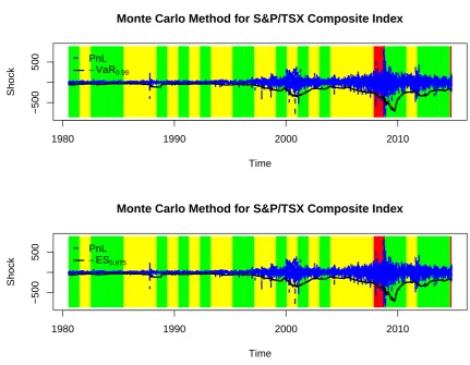
Figure 2.5: The Monte Carlo method for S&P/TSX Composite Index where 99% VaR and 97.5% ES are calculated to compare with PnL. The darkest bar represents the red zone, the lightest bar represents the yellow zone and the rest represents the green zone.
Figure 2.4, the Monte Carlo method gives more breaches of VaR and ES but a smaller amount of reserve capital (see in Figure 2.5). From the perspective of the regulators, they are more concerned with the number of breaches so as to avoid systemic risk3.
Although the Monte Carlo method is regarded as the better theoretical approach, it suffers from two main problems. One of them is the computational complexity. For example, for each risk factor, 100,000 simulated scenarios could be generated. As a result, the running time for a portfolio including thousands of factors is unacceptable. So in practice sampling for a longer period is often applied (Glasserman, 2003). Another problem is misspecification of the underlying process. The remedy could rely on one’s prior experience and trial-and-error for new assumptions and models.
3Systemic risk refers to the risk that an event triggers a collapse of the financial system, whereas systematic
2.2
Kernel Methods
As described above, financial risk managers are concerned with the distribution of risk factors, estimation of parameters or how these risk factors vary over time for the purpose of managing market risks.
To estimate the distribution, one can assume a specific form for the variables and validate the assumption by some criterion. For example, changes to the logarithm of the stock prices are usually assumed to be normally distributed, so graphical techniques (e.g. histogram and Q-Q plot) or statistical test (e.g. Jarque-Bera test and Shapiro-Wilk test) can be used to determine the normality of the distribution. To estimate the parameters, one can specify the model first, apply the maximum likelihood method and finally test the validity of the assumption. For example, the interest rate is supposed to follow the square-root CIR process but many researchers devote a great deal of attention to studying the plausible form of the drift and diffusion (Andersen and Lund, 1997; Conley et al., 1997; Chapman et al., 1999; Ang and Bekaert, 2002). To forecast future values, one can use the ARMA-GARCH model to fit the data and then make prediction based on the model, but the linearity or nonlinearity of the terms must be tested when the model is used.
Parametric methods as described above cannot avoid the problem of misspecification. Al-though changes to the logarithm of the stock prices are assumed to be normally distributed, these log returns are often observed to be skewed and to have fat tails. As a result, this mis-specification may result in large estimation bias and the assumption of log-normality could be violated. In this case, one has to propose a new assumption and test it again. Also, except the CIR model and other descriptions of the dynamic, the actual forms to characterize the short-term interest rate are still on exploration. This trial-and-error process largely depends on one’s prior experience. Therefore it is more or less inevitable to use the wrong form by parametric methods.
In such cases, the nonparametric technique could be an alternative to its parametric coun-terpart. One of its advantages is that instead of requiring prior information on specifying the parametric form, the technique lets the data speak of the appropriate functional form so that misspecification can be avoided. This is why nonparametric regression has received grow-ing attention from academia and industry. But the nonparametric technique is not a panacea because they do result in higher computational costs. In addition, some criticize that the meth-ods are “black-box” and lack intuitive interpretation. In fact, nonparametric and parametric methods are complementary to each other from a practical perspective.
2.2. KernelMethods 13
smoothing splines, kernel regression is easy to implement and popular in real applications. So this thesis mainly focuses on kernel-type estimators.
2.2.1
Kernel Density Estimators
As mentioned above, one of the concerns with density estimation in finance is related to char-acterizing tail events such as calculation of VaR or ES. So in this part density estimation by kernel methods is introduced.
Suppose that the data X1,X2, . . . ,Xn come from a common density function f. We know
that the distribution function F(x) is equal toP(X ≤ x), so the empirical distribution function is expressed as
ˆ
Fn(x)=
1
n n
∑
i=1
I(Xi ≤ x)
where I(·) is the indicator function. If it is also assumed that X is continuous, then F(x) =
∫ x
−∞ f(u)du, that is, f(x) = dF(x)/dx. Thus we can use an empirical distribution function to
derive the estimator of the density, that is, for a small positive constanthn
ˆ
fn(x)=
ˆ
Fn(x+hn/2)−Fˆn(x−hn/2)
hn
= 1
nhn
n
∑
i=1
I(|Xi−x| ≤hn/2)
By lettingK(x)= I(|x| ≤1/2), the above expression is rewritten as
ˆ
fn(x)=
1
nhn
n
∑
i=1
K
(
Xi−x
hn
)
(2.5)
Herehn is called the bandwidth (or smoothness parameter) andK(·) is called the kernel
func-tion. In addition to the uniform kernel K(x) = I(|x| ≤ 1/2), we can also take other forms for K(·), which results in different estimators. Informally, K(·) is the kernel function from
R to R which satisfies ∫−∞∞ K(x)dx = 1. K(·) is non-negative if K(x) ≥ 0 and symmetric if
K(x)= K(−x). The j-th moment ofK(·) is defined asmj =
∫∞
−∞xjK(x)dxand the order ofK(·)
is defined as inf{j:mj ,0}. For example, ifm1 =0 andm2 > 0, thenK(·) is a second-order
k-ernel. It can be verified that the Gaussian kernelK(x)= √1
2πe
−x2/2
is a symmetric, non-negative and second-order kernel function; this kernel is commonly used in practice. The Epanechnikov kernelK(x)= 34(1− x2)
+is also commonly used in real applications.
2.2.2
Kernel Regression Estimators
used to assist interpolation and extrapolation for missing data in some data sources.
Given the data (X1,Y1),(X2,Y2), . . . ,(Xn,Yn), the simple linear regression model is given by
Yi =β0+β1Xi+εi
whereβ0, β1 are parameters, and the errorsε1, ε1, . . . , εn satisfy E(εi) = 0 and Var(εi) = σ2.
More generally, one would like to specify nonlinear relationships such as the exponential or logarithm function between X and Y. But as mentioned above, it is rare to know the true functional form in real applications, so lack of prior information could lead to inconsistent estimation by the presumed model. Nonparametric regression avoids this problem by freeing the assumption of the functional form about the data generation process. In the nonparametric regression model, we are concerned about estimation ofg(x) such that
Yi =g(Xi)+εi (2.6)
whereg(·) satisfies some regularity conditions such as smoothness and moment conditions. We can use Taylor expansion to approximateg(Xi) in a neighborhood of x
g(Xi)=g(x)+(Xi−x)g′(x)+
1
2(Xi−x)
2g′′(x)+o(|X
i−x|2
)
The functional form ofg(·) is usually unknown, so by lettingβj,xdenote the estimate of the j-th
order derivative of g(x), kernel regression uses the weighted least squares technique to fit the data at the neighborhood of xby a polynomial of degree p, which minimizes
n
∑
i=1
Yi −
p
∑
j=0
βj,x(Xi− x)j
2
Khn(Xi−x) (2.7)
where Khn(x) = K(x/hn)/hn. Thus the estimator ˆβ0,x gives the estimated value of g(x), and similarly we can approximate the j-th order derivative ofg(x) by ˆβj,x.
Moreover let Y = Y1 Y2 ... Yn
X =
1 (X1− x) . . . (X1−x)p
1 (X2− x) . . . (X2−x)p
· · · ·
1 (Xn− x) . . . (Xn−x)p
βx =
β0,x
β1,x
... βp,x
(2.8)
andWx = Diag{Khn(X1 −x),Khn(X2− x), . . . ,Khn(Xn− x)}, then the least-squares estimate to
(2.7) atxis given by
ˆ βx =
(
XTWxX
)−1
2.2. KernelMethods 15
thus the estimator ofg(x) is
ˆ
gn(x)=eT1βˆx =eT1
(
XTWxX
)−1
XTW Y
whereeT
1 =(1,0, . . . ,0)
T. When p= 0 in (2.7), the estimator is reduced to be locally constant
(also known as the Nadaraya-Watson estimator) proposed by Nadaraya (1964) and Watson (1964), which can be rewritten as
ˆ
gn(x)=
n
∑
i=1
YiKhn(Xi− x)
n
∑
i=1
Khn(Xi− x)
(2.10)
The local linear estimator, i.e. p=1 in (2.7), is proposed by Fan (1993) with the closed form
ˆ
gn(x)=
n
∑
i=1
wiYi
n
∑
i=1
wi+n−2
wherewi =K(x−Xi
hn
)
[sn,2−(x−Xi)sn,1] with
sn,j =
n
∑
i=1
K
(
x−Xi
hn
)
(x−Xi)j
For general p, there is no such closed form for ˆgn(x). Fan and Gijbels (1996) gave a detailed
study of this general case but advocated that the local linear estimator is enough in practice. Moving beyond the local constant and local linear estimators, Hall et al. (1999) and Cai (2002) proposed a weighted Nadaraya-Watson estimator given by
ˆ
gn(x)=
n
∑
i=1
pi(x)YiKhn(Xi−x)
n
∑
i=1
pi(x)Khn(Xi−x)
wherepi(x) are weights and satisfy: (1)pi(x)≥ 0; (2)∑ni=1 pi(x)= 1; (3)∑ni=1pi(x)Khn(Xi−x)= 0. Hall et al. (1999) and Cai (2002) proved that the weighted Nadaraya-Watson estimator and the local linear estimator have the same asymptotic distribution.
domain, which is so called the boundary effect. To overcome this problem, many methods have
0.0 0.2 0.4 0.6 0.8 1.0
−0.3
−0.2
−0.1
0.0
0.1
The Nadaraya−Watson Estimator
x
y
0.0 0.2 0.4 0.6 0.8 1.0
−0.3
−0.2
−0.1
0.0
0.1
The Local Linear Estimator
x
y
Figure 2.6: Boundary effect for the Nadaraya-Watson estimator and the local linear estimator, where the data are generated byy=−(x−0.5)2+0.05εwithε∼ N(0,1). The solid line is the true curvey= −(x−0.5)2, and the dotted line gives the fitted values.
been proposed to remove the boundary bias such as the geometrical method (Hall and Wehrly, 1991) and the boundary correction approach (Gray and Schucany, 1972; Rice, 1984). In ad-dition, the local linear estimator and the weighted Nadaraya-Watson estimator as mentioned above have automatically boundary adaption (see in Figure 2.6).
2.2.3
Choice of Bandwidth and Kernel Function
Relative to the kernel function, the choice of the bandwidth hn is critical to the performance
of the estimator (Wand and Jones, 1995). From the definition of the kernel function, it can be found that the bandwidth controls how many sample points are included in estimation. In fact, there is a tradeoffbetween bias and variance (see Figure 2.7). Largerhnwill include more sample points such that the estimator is not sensitive to the randomness, so the variance can be reduced. But in this case the estimator tends to be further away from those local points, as a result there is a larger bias. Similarly smallerhn will result in smaller bias but larger variance.
So it is very important to have a reliable choice of bandwidth which trades offbetween these two extremes.
corre-2.2. KernelMethods 17
20 30 40 50 60
12
13
14
15
Bandwidth = 0.5
Age
Log(W
age)
20 30 40 50 60
12
13
14
15
Bandwidth = 1.0
Age
Log(W
age)
20 30 40 50 60
12
13
14
15
Bandwidth = 5.0
Age
Log(W
age)
20 30 40 50 60
12
13
14
15
Bandwidth = 10.0
Age
Log(W
age)
Figure 2.7: Four Nadaraya-Watson estimators for Canadian male wage data on 1971, where the bandwidth arehn =0.5,hn =1.0,hn =5.0 andhn =10.0.
spond to a variety of estimators, and the goal of CV is to validate how accurately the estimator will perform in real applications, so one can use CV to choose the optimalhn based on some
(2.6), each time the leave-one-out CV uses one observation as the testing dataset and the re-maining as the training dataset, and repeats until each observation is used to test (see Figure 2.8). In other words, given the fixed bandwidthhn, let ˆY−idenote the fitted value onXiobtained
by the trained model without considering Xi, i.e. ˆY−i = gˆn,−i(Xi) where ˆgn,−i(x) is constructed
on the entire dataset excluding (Xi,Yi). For the case of the Nadaraya-Watson estimator, ˆgn,−i(x)
is given by
ˆ
gn,−i(x)=
n
∑
j=1 j,i
YjKhn(Xj− x)
n
∑
j=1 j,i
Khn(Xj− x)
After that, the optimal bandwidth is chosen as
hoptn = arg min hn
n
∑
i=1
(Yi−Yˆ−i)2
In addition, the leave-one-out CV can be generalized to the leave-p-out CV (Shao, 1993; Zhang, 1993), and partial data splitting schemes have been proposed in practice including
k-fold CV introduced by (Geisser, 1975).
20 30 40 50 60
12
13
14
15
Age
Log(W
age)
0.0 0.2 0.4 0.6 0.8 1.0
−0.3
−0.2
−0.1
0.0
0.1
x
y
Figure 2.8: The leave-one-out CV is performed on the same Canadian male wage data seen in Figure 2.7 (left) andy= −(x−0.5)2(right). The optimal bandwidth ishoptn =1 for the left and hoptn =0.01 for the right.
2.2. KernelMethods 19
kernel is used, then it can be calculated that
Bias[ ˆfn(x)] =
1
l!f
(l)(x)hl
nml+o(hln)
Var[ ˆfn(x)] = f(x)
∫
RK
2(u)du
nhn +O ( 1 n )
which leads to the asymptotic mean squared error (AMSE) given by
AMSE[ ˆfn(x)]=
[
1
l!f
(l)
(x)hlnml
]2
+ f(x)
∫
RK
2(u)du
nhn
with this definition the asymptotic mean integrated squared error (AMISE) can be calculated as
AMISE[ ˆfn(x)]=
∫
R
AMSE[ ˆfn(x)]dx=
[
hl
nml
l!
]2∫
R
[f(l)(u)]2du+
∫
RK
2(u)du
nhn
Note that the above AMISE is a function ofhn, which implies that the optimalhn can be taken to minimize the AMISE. By taking the derivative of AMISE with respect tohnand setting it to
zero, we have
hoptn =
(l!)2∫RK2(u)du
2lm2
l
∫
R[f
(l)(u)]2du
1/(2l+1)
×n−1/(2l+1)
It is noted thathoptn is related to
∫
R[f
(l)(u)]2dubut f(x) is an unknown function. So Silverman
(1986) suggested to use a plausible candidate such as the normal density to replace f(x). This results in the rule-of-thumb for the bandwidth hoptn = Cσˆn−1/(2l+1) whereC is some constant
and ˆσ is the sample standard deviation. If the standard normal kernel is used, the optimal bandwidth is ˆσn−1/5.
Note that given the number of observationsn, the bandwidth in (2.7) is constant, neither incorporating the location of x nor that of Xi. As Fan and Gijbels (1996) pointed out, this
constant bandwidth may not estimate curves with a complicated shape very well. Thus they introduced variable bandwidthh/α(Xi) such that (2.7) can be written as
n
∑
i=1
Yi−
p
∑
j=0
βj(Xi−x)j
2
Khn/α(Xi)(Xi−x)
whereα(·) is positive and reflects the difference of each data point. Then AMISE is minimized to obtain the optimal bandwidth hn and α(·). They found that by using variable bandwidth,
Recently the choice of kernel functions has also been studied because it is found that clas-sical methods with symmetric kernels have significant bias errors on the boundary (Mackenzie and Tieu, 2004). Michels (1992) used an asymmetric gamma kernel function to reduce the bias in estimation, and found that the use of asymmetric kernels can lead to better predictions in a time series model for environmental data. Chen (2002b) used asymmetric kernels in local lin-ear regression and claimed that the flexible shape of asymmetric kernels supplies advantages of having finite variance and resistance to sparse design. Abadir and Lawford (2004) studied the class of optimal asymmetric kernels in the sense of the mean integrated squared error (MISE) and analyzed its main properties.
1980 1990 2000 2010
−1000
0
Kernel Density Estimation for S&P/TSX Composite Index
Time
Shock
PnL
−VaR0.99
1980 1990 2000 2010
−1000
0
Kernel Density Estimation for S&P/TSX Composite Index
Time
Shock
PnL
−ES0.975
Figure 2.9: Historical simulation for S&P/TSX Composite Index where daily shocks are used for demonstration and 99% VaR and 97.5% ES are calculated to compare with PnL. All trading days are in green zone.
2.3
Example
2.3. Example 21
ES is to predict the PnL distribution, so the kernel density estimator (2.5) can be used to fulfill the task. For illustration, historical simulation with the same parameters as in Figure 2.4 is used to generate the predicted shocks. Then instead of (2.3) and (2.4), we apply (2.5) to estimate the density of these shocks and make use of the original definition (2.1) and (2.2) to find VaR and ES. Figure 2.9 illustrates this application. It is noted in this case that for comparison with Figure 2.4, the results given by the kernel density estimator are more conservative as there are no breaches in the whole period. But we must admit that financial institutions might not be satisfied with these results because they imply higher capital requirements and so a lower return on equity.
Literature Review
In the last few decades, nonparametric regression has attracted growing attention from a-cademia and industry because it requires little prior information on the process which gen-erates the data. Nonparametric estimation for continuous-time models has been studied for many years (Tuan, 1981; Rao, 1985; Soulier, 1998; Spokoiny, 2000; Papaspiliopoulos et al., 2012), but the assumption of continuous time is unreasonable in real applications. Therefore the purpose of this chapter is to review recent developments of nonparametric regression based on discrete-time observations for estimation of the drift and diffusion in stochastic diff eren-tial equations (SDEs). For those wishing a review, a brief introduction of SDEs, in particular diffusion processes, is provided in Appendix A.
3.1
Time-Homogeneous Di
ff
usion Models
Florens-Zmirou (1993) left the drift restriction-free and proposed the following kernel estima-tor for the time-homogeneous diffusion by using the uniform kernel
ˆ
b2n(x)=
n∑−1
i=1
I(|Xi−x|<hn)n(Xi+1−Xi)2
n
∑
i=1
I(|Xi−x|<hn)
For high-frequency data, i.e. in the limit as the discretization step size tends to zero, the au-thor proved quadratic convergence and asymptotic normality of the estimator by expanding the transition density. By assuming the mean-reverted drift, A¨ıt-Sahalia (1996) proposed a non-parametric estimator for the diffusion in the time-homogeneous case by using the Kolmogorov forward equation with time-stationary transition density, i.e. ∂p(Xt+h|Xt)
∂t = 0, where p(Xt+h|Xt)
is the transition density of Xt+h given Xt in (A.5) in Appendix A. The Kolmogorov forward
3.1. Time-HomogeneousDiffusionModels 23
equation can yield
b2(Xt)= 2
p(Xt)
∫ Xt
0
a(y)p(y)dy
where p(y) is the stationary density function of the time series{Xt} and can be approximated by the kernel density estimator as mentioned in Chapter 2. Note that the Kolmogorov forward equation with the time-stationary transition density can also provide a relationship
a(Xt)=
1
p(Xt)
d
dXt
[b2(Xt)p(Xt)] (3.1)
so Jiang and Knight (1997) first proposed a kernel estimator ofb2(x) given by
ˆ
b2(x)=
n∑−1
i=1
(Xi+1−Xi)2
△ Khn(Xi−x)
n
∑
i=1
Khn(Xi−x)
.
Based on (3.1) an estimator ofa(x) is proposed by
ˆ
a(x)= 1
p(x)
d
dx[b
2
(x)p(x)]= 1 2
[
dbˆ2(x)
dx +bˆ
2
(x)pˆ
′(x)
ˆ
p(x)
]
where ˆp(x) is the estimator of the density function given by 1n∑ni=1Khn(Xi−x). The central limit theorems for ˆa(x) and ˆb2(x) are established and valid conditionally on the path passing through
x. The methods are also applied to estimation of the short-term interest rate. Arapis and Gao (2006) specified Jiang and Knight’s method by using a Gaussian kernel function to derive the closed form of the estimators ofa(x) andb2(x).
Stanton (1997) applied the infinitesimal generator (Øksendal, 2003) of the time-homogeneous diffusion model to expand the function f(t,Xt) oftandXt, where
Lf(t,x) = lim
τ↓t
E(f(τ,Xτ)|Xt = x)− f(t,x)
τ−t =
∂f(t,x)
∂t +a(x)
∂f(t,x)
∂x +
1 2b
2(x)∂
2f(t,x)
∂x2 .
ThenE[f(t+△,Xt+△)|Xt] can be expressed in the form of a Taylor expansion
E[f(t+△,Xt+△)|Xt]= f(t,Xt)+△Lf(t,Xt)+ 1
2△
2L2
f(t,Xt)+· · ·+ 1
n!△
nLn
f(t,Xt)+O(△n+1)
Then the first and second order approximations are
Lf(t,x) = 1
△E[f(t+△,Xt+△)− f(t,Xt)|Xt = x]+O(△) Lf(t,x) = 1
2△{4E[f(t+△,Xt+△)− f(t,Xt)|Xt = x]−E[f(t+2△,Xt+2△)− f(t,Xt)|Xt = x]}+O(△
By taking f(t,x) = x, implyingLf(t,x)= a(x), first and second order approximations ofa(x) are
˜
a(x) = 1
△E[Xt+△−Xt|Xt = x]+O(△)
˜
a(x) = 1
2△{4E[Xt+△−Xt|Xt = x]−E[Xt+2△−Xt|Xt = x]}+O(△
2).
By taking f(t,x) = (x−Xt)2, implyingLf(t,x) = 2a(x)(x−Xt)+b2(x) soLf(t,Xt)= b2(Xt),
first and second order approximations ofb2(x) can be given by
˜
b2(x) = 1
△E[(Xt+△−Xt)2|Xt = x]+O(△)
˜
b2(x) = 1
2△
{
4E[(Xt+△−Xt)2|Xt = x]−E[(Xt+2△−Xt)2|Xt = x]
}
+O(△2),
where ˜a(x) and ˜b2(x) can be estimated using data Xi,i = 0, . . . ,n. Stanton applied the above
methods to estimate the drift and diffusion of the short-term rate and the market price of the interest rate risk by using the daily three- and six-month treasury bill data. The author claimed that higher order estimation should outperform lower order estimation. However, Fan and Zhang (2003) found that this claim may not always hold true. They extended Stanton’s method and gave the general high order estimation of the drift and diffusion coefficients by adding weights
Lf(t,Xt)=
1
△ k
∑
i=1
ak,iEt[f(t+i△,Xt+i△)− f(t,Xt)]+O(△k)
whereak,i = (−1)i+1
(k
i
)
/i. Then local polynomial regression is used to derive the estimator of
a(x) andb2(x), and the asymptotic behaviors are obtained. They found that the asymptotic
bias-es of the higher order bias-estimators can be reduced but the asymptotic variancbias-es increase with the order of the estimator. However, the nonnegativity of the local linear estimator of the diffusion cannot be guaranteed, so some researchers proposed different methods to overcome this short-coming of local polynomial estimation. One method is through logarithmic transformation to retain nonnegativity (Ziegelmann, 2002), i.e. the estimator of the diffusion is given by
( ˆβ0,βˆ1)= arg max
β0,β1
n−1
∑
i=1
[
(Xi+1−Xi)2
△ −eβ0+β1(x−Xi)
]2
Khn(x−Xi)
Similar ideas can be also found in (Yu and Jones, 2004). In Yu and Jones’s method, one can use the Euler scheme to approximate the time-homogeneous case by (A.8), that is,
Xi+1= Xi+a(Xi)△i+b(Xi)
√
3.1. Time-HomogeneousDiffusionModels 25
LetYi =Xi+1−Xi, then the likelihood function for the process (3.2) is written as
n−1
∏
i=1
1
√
2πb2(Xi)△i exp
{
−[Yi−a(Xi)△i]2
2b2(X
i)△i
}
and the log-likelihood function is proportional to
n−1
∑
i=1
[
log(b2(Xi)△i)+
(Yi−a(Xi)△i)2
b2(X
i)△i
] .
By letting a(Xi) = α0 +α1(x− Xi) and logb2(Xi) = β0+β1(x− Xi), one can propose kernel
estimators of the drift and diffusion and use optimization procedures to determine the parame-tersα0, α1, β0andβ1. Note that the above logarithmic transformation can retain nonnegativity
of the estimator of b2(x). But the transformation introduces an extra bias such that the
re-sulting estimators may not have closed-form representation. Cai (2001) proposed a weighted Nadaraya-Watson estimator to capture both advantages from local constant and local polyno-mial methods by defining the weights
wi(x)≥0
n
∑
i=1
wi(x)=1 and
n
∑
i=1
(Xi−x)wi(x)Khn(x−Xi)= 0
so one can use the weighted version of the Nadaraya-Watson method to estimate the diffusion by
ˆ
b2(x)=
n∑−1
i=1
wi(x)Khn(x−Xi)
(Xi+1−Xi)2
△
n
∑
i=1
wi(x)Khn(x−Xi)
then the constrained optimization technique is used to determine the weights. Xu (2010) ex-tended Cai’s method in more general settings. In addition, Arfi (2008) proved that the estima-tors by Stanton (1997) have strong consistency under some regular conditions.
For low-frequency data, with the fixed discretization step size, Nicolau (2003) quantified the bias of the Florens-Zmirou (1993) and Jiang and Knight (1997) estimators for the diffusion in the time-homogeneous case. Meanwhile, based on the quantified bias, Nicolau proposed a bias adjustment method to partially attenuate the distortion. In addition, weak consistency and asymptotic normality are obtained for the estimators. Gobet et al. (2004) proposed kernel estimators of the drift and diffusion under the assumption of ergodicity and proved quadratic convergence by the spectral analysis of the associated Markov semigroup.