Coordinate Systems, Numerical Objects and Algorithmic
Operations of Computational Experiment in Fluid Mechanics
Alexander Degtyarev1,aand Vasily Khramushin1,b
1St. Petersburg State University, Universitetskii prospect 35,198504 Saint-Petersburg, Russia
Abstract. The paper deals with the computer implementation of direct computational experiments in fluid mechanics, constructed on the basis of the approach developed by the authors. The proposed approach allows the use of explicit numerical scheme, which is an important condition for increasing the efficiency of the algorithms developed by numerical procedures with natural parallelism. The paper examines the main objects and operations that let you manage computational experiments and monitor the status of the computation process. Special attention is given to a) realization of tensor repre-sentations of numerical schemes for direct simulation; b) realization of representation of large particles of a continuous medium motion in two coordinate systems (global and mobile); c) computing operations in the projections of coordinate systems, direct and in-verse transformation in these systems. Particular attention is paid to the use of hardware and software of modern computer systems.
1 Introduction
The problems of the Computational Fluid Dynamics (CFD) are among the most complex for imple-mentation on modern computers both because of their strong connectivity and because of the complex nature of the problem. Not surprising that a large number of “grand challenges” to one degree or an-other gets reduced to CFD problems.
Traditionally, the calculation of flows is associated with the solution of Navier-Stokes equations. The problems in this area can be divided into three broad groups [1]:
1. Incorrectness of the Navier-Stokes equations underlying the simulation, since it is a certain idealization of real processes.
2. Idealization is also present in the geometry of these flows. This concerns sharp edges, corners, etc. in calculations. Such ideal forms were due to the method of approximation using large meshes. This causes a very big problem in the solution, because in reality most of these features are absent. Currently, the size of the mesh may be significantly reduced, which means that the methods of dealing with the problems that arise should be different.
3. Every time when the current problems are mapped on a new computer architecture, there arise porting problems of such applications. Since long ago it became clear that the appearance of
new architectures is related with the appearance of new programming environments, which means the development of new libraries for currents will also be needed. Thus, we need to approach the problem of fluid dynamics programming in a different way.
A distinctive feature of the solution of the first problem is the traditional use of the implicit nu-merical schemes. Such a way reduces the solution to linear algebra problems that do not allow to efficiently control nonstationary processes and qualitative changes of the continuum for the consid-ered complex problem. Moreover, the disadvantage of the implicit schemes as compared with the explicit ones is in the raise of complexity and parallelization problems. We know that it is a price to pay for the stability of the numerical scheme. However, the attractiveness of the explicit schemes has led to the development of an approach based on the description of the behavior of many large liquid particles [2]. Problems of numerical schemes instability in this case are avoided by providing a large particle with additional degrees of freedom. Geometrically this requires the introduction of a dual basis for describing the state of a large particle [3], [4].
The second group of problems is connected just with the geometric description of these flows. The efficiency of the calculations (especially in the case of direct numerical schemes) depends sig-nificantly on the description of the modeled objects, computational meshes and possibilities of their transformation and manipulation [5], [6]. This article is focused on the construction of such formal computational basis. Special attention is paid to programming procedures, which take into account the architecture of the computing systems.
2 The subject of application
The algorithmic realization of direct numerical simulations using explicit schemes has a beautiful his-torical analogy [2] in the form of calculus of fluxions by Isaac Newton. In the up-to-date algorithms, such implementation is represented as three-dimensional space numeric objects. Between them, con-nections are established for hydromechanics laws implementation.
Fluxions calculus1creates the basis of Newton classic mechanics for the motion in vector space and scalar time. VelocityV [m/s] becomes first fluxia in kinematics. It is differential (in accordance with Newton “moment”) in multiplication with time stepΔt[s] or justt. If we adapt such reasoning with reference to modern algorithms, then motion of control point in space is presented as follows2:
+→−A =→−R+→−V·t+←a−·(∧r+v∧·t)=0→−A+(→−V +←a−·∧v)·t, (1)
wheretis the calculated time interval [s];←−a is the vector count in the local basis (of the large particle) [m−2];+→−Aand0→−Aare new and initial positions of the control point in the global reference system [m]; −
→
R is the location of the local basis in the global reference system [m];→−V is the velocity of the local basis translational displacement [m/s];v∧[m3/s] is the tensor of rotation and deformation of the basis axes of the tensor form3∧r[m3].
This equation presents a point shift during one step of the direct computational experiment. As shown, it can be represented in the form of the recalculation from the local coordinates of the point into the global reference system in accordance with the time intervalt.
1fluens, fluentisare functionsx, y,zon the argument of timet;fluxiox˙,y,˙z˙are time derivatitivesx, y,z.
2In scalar notation: +Ax=0A
x+(Vx+vxxax+vxyay+vxzaz)·t; +Ay=0A
y+(Vy+vyxax+vyyay+vyzaz)·t; +Az=0A
z+(Vz+vzxax+vzyay+vzzaz)·t.
Renewed spatial field of velocities and deformations are used at conjugate stage of computational experiment. They are necessary for the control of the dynamic state as well as for redefining rheolog-ical characteristics of fluid, which are presented in the form of scalar, vector and tensor objects. In up-to-date complex computational models similar hydrodynamic characteristics are associated with spatial distribution of polarized dipole cores, initiated sources of vortexes, etc.
Obviously, the direct computational experiment efficiency directly depends on the manipulation efficiency with reference systems, numerical objects and algorithmic operations on these objects.
3 Geometric synthesis of computational objects and related algorithmic
operations
Let us consider the principles of construction of the computational objects in direct computational experiment. The described approach allows to partly automate the validation of code writing and to improve its computational efficiency.
The geometrical construction of spatial problems includes scalar, vector and tensor numerical ob-jects. Algorithmic procedures and arithmetic-logic operations are defined in the dimensional physical form and associate numerical objects and interpolation basis in a tensor mesh space.
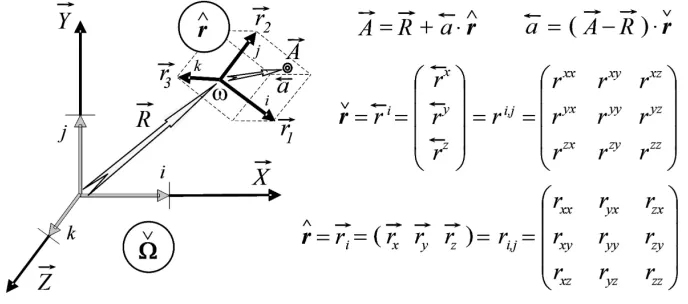
Figure 1. Geometry of global space (Ω∨) and local basis (∧r(ω));i,j,kdenote unitary vectors in the connected reference system
Elementary numerical objects are formed by non-coplanar basis vectors (Fig. 1). They serve to build indissoluble physical fields in the vicinity of adjacent mesh nodes (TΩ→−R) and centers of mass (ω). Products of vector and tensor quantities are performed with convolution, i.e. by summation over a repeated index in the monomial product (←−a =→−a·∨roraj =a
i·ri j), the transition to local basis and back (→−a =←−a·r∧orak=aj·rjk). The latter occurs at the return to absolute coordinates.
The proposed notation is similar to that in [7] and [8]. The symbol notations and the principles of their construction are summarized below.
– A Left low index marks a location in the mesh space{X,Y,Z} ∧r, or links to adducent knots{+} ∧r, or centers of mass of liquid particles{−}∨r. It is performed on conjugate stages of the computational experiment.
Right indices connect vector and tensor components in absolute and local bases. They serve to a strict definition of the dynamics and deformation of numeric cells (particles of a continuous medium). – Low right indices, tensor “box” and the right arrow show the belonging to an absolute coordinate
system (Fig. 1). For example, the tensor∧r[m3] is a collection by columns of basis vectors→−r i in matrices of geometric transformations (like→−a =←−a·∧r[m]).
– Upper right indices mark projections inside mobile and deformable mesh cells. The display of unitary vectors of absolute coordinates lies in row vectors in matrix of inverse coordinate
transforma-tions,∨r= ←r−j = rjk =∧r−1 [m−3]. They are marked by tensor “tick” and vector left arrow←−a =→−a· ∨r [m−2].
– Capital letters are used for big numerical values measured in scale of global space (Ω) and general absolute time (T);
– Lowercase letters are used for especially small quantities or finite differences which are com-mensurable with the physical dimensions of local bases of particle continuumω, as well as in the range of the current time stept.
The absolute timeT can contain the Julian date and time from the beginning of the day4: kT = T +k·t. Absolute values in space may also be presented5:→−A =→−R +←−a· ∧r[m] (geographical and other generalized coordinates). The need of involvement of absolute encoder in spaceT
Ω→−R and time Tis eliminated in the balanced numerical schemes. In this case, the use of numerical values at nodes and centers of mass of conjugate mesh cells is sufficient at all stages of calculations∧r[m3].
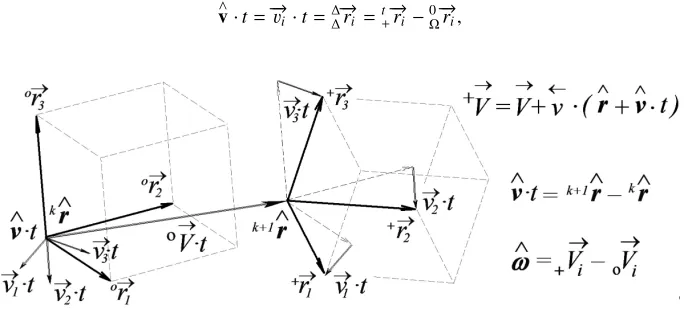
Kinematics of internal streams is defined by the speed difference tensor (Fig. 2). It is given on the large liquid particles basis vectors form shifted in time,
∧
v·t=→−vi ·t=ΔΔ→−ri =t+→−ri−0Ω→−ri, (2)
Figure 2.Movement of basis vectors of calculation cell in space
4The real time is set by the numeric structureEventwith Julian data:D(from 4713 BC), and local time in hours from the day beginning:T.
The tensor∧v[m3/s] defines the current speed of the displacement of the liquid particle basis vectors on a local scale (lowercase letters) that is measured in the projection of the global coordinate system (lower indices). The independent convective rates tensor describing the local motion of the fluid is obtained after transformation of the velocity tensor reference frame6 to the local basis of the large liquid particle (geometric normalization):<v=∧v·∨r[1/s].
The tensor (v<[1/s]) contains the extended set of kinematic elements of the differential equations with cross derivative components of deformable liquid particle motion:
<
v=∧v·∨r=vi jrjk= ⎛ ⎜⎜⎜⎜⎜ ⎜⎜⎜⎝ vxxr
xx+v
xyryx+vxzrzx vxxrxy+vxyryy+vxzrzy vxxrxz+vxyryz+vxzrzz vyxrxx+vyyryx+vyzrzx vyxrxy+vyyryy+vyzrzy vyxrxz+vyyryz+vyzrzz vzxrxx+vzyryx+vzzrzx vzxrxy+vzyryy+vzzrzy vzxrxz+vzyryz+vzzrzz
⎞ ⎟⎟⎟⎟⎟ ⎟⎟⎟⎠. (3)
Alternatively, such products can be presented in the form of complete differentiationv<=v∧ / ∧r= Δ
ω→−vi/Δω→−riexecuted without artificial exceptions of “small” or convective elements in substantial deriva-tive approximations. Thus correct physical interpretation of rheological characteristics of liquid and living conditions of currents is remained.
4 Construction of tensor numerical objects and modeling algorithms
Computing space is constructed on fixed nonregularized nodes (Point) in indexed set of mesh cells. Three-dimensional interpolation is carried out using Euclidean bases (Base). Inside and in the vicin-ity, coordination of physical laws with the use of free vectors (Vector) is realized.
Object-oriented programming allows to move the control of the basic math operations correctness at the stage of the source program compilation, if they are applied to uniquely determined numerical objects (in accordance with physical characteristics).
The main computational objects (see, e.g., [9]) are defined by the requirement of fast and indepen-dent performance of computational operations. Particular attention is paid to the possibility of quick adjustment of the calculations for the application of hybrid algorithms depending upon conditions of the physical phenomena existing in a local subdomain. The following objects are introduced:
typedef doubleReal; //scalar quantity in global space and time
typedef doublereal; //local or differential counts in space and time
structTensor; //tensor object without contextual links for quick calculation
structBase; //location coordinates and related Euclidean basis
structCell; //numerical cell with contextual links to adjacent particles
structPoint; //point in scale of absolute reference system
structVector; //free difference vector in scale of local reference system
structSpace; //space of nodal elements for net area in general
structVolume; //set of free/moving and deformable cells
The control of the correctness of the mathematical operations with respect to the listed objects can be illustrated as follows. The automatic conversion of a complex variableVectororTensorto a local valuerealdetermines the length of the vector and the determinant of the matrix. Any other transformation are marked as wrong by a translator. The difference between values of typePointcan
6Prohibition improving rank in product operation enables automatic permutation of factors in geometric transformations:
∧
only give a value ofVector. Addition of objects of typeVectorwithVectororPointvalues will result in the same type of data, and no other.
The development of modern computers goes rather towards adding more RAM, than towards im-proving the processing of large amounts of data. The basic data arrowsSpaceandVolumehave to be retained at current, previous and subsequent cuts in time for the technical support of the paral-lelization. This allows to synchronize the parallel processing in the case of complete separation of the stages of the experiment into independent physical processes, or to create any cycles for matching parameters of the computing environment in complex and ill-conditioned mathematical models, if necessary.
5 Conclusion
The solution of any computational problem consists of several stages: – problem identification;
– formalization of the physical problem; – construction of a computational procedure;
– creation of code for the chosen computer architecture.
At the transition between any successive stages, qualitative change in the essence of the described phenomenon can occur. Problems associated with incorrect mathematical models, numerical schemes to replace them, mapping problems on the architecture of a computer system, etc. are quite well known. For an adequate creation of a complete solution of the problem, it is necessary to develop consistent mapping of one stage onto another. The above approach is an attempt to adequately repre-sent the final stage of solving the overall problem.
Acknowledgements
The research was carried out using computational resources of Resource Center Computer Center of Saint-Petersburg State University and supported by Russian Foundation for Basic Research (project N 13-07-00747) and St. Petersburg State University (projects N 9.38.674.2013, 0.37.155.2014).
References
[1] A. V. Bogdanov, A. B. Degtyarev and V. N. Khramushin, Computer Research and Modeling7, 3, 429–438 (2015)
[2] A. B. Degtyarev and V. N. Khramushin, Mathematical Modeling26, 11, 4–17 (2014)
[3] V. N. Khramushin, Vestnik of Saint-Petersburg University, Series 10 : Applied Mathematics. Computer Science. Control Processes, 2, 108–117 (2015)
[4] V. N. Khramushin,3D Tensor Mathematics for the Computational Fluid Mechanics Experience
(FEB RAS, Vladivostok, 2005)
[5] I. D. Faux and M. J. Pratt,Computational Geometry for Design and Manufacture (Mathematics
and Its Applications)(Ellis Horwood, 1981)
[6] A. J. McConnell,Applications of Tensor Analysis(Dover Publications, 2011)
[7] G. Astarita and G. Marrucci, Principles of Non-Newtonian Fluid Mechanics (Mc Graw-Hill, 1974)