Feynman Paths and Weak Values
R. Flack, B. J. Hiley
Department of Physics and Astronomy, University College London, Gower Street, London WC1E 6BT.
Abstract: There has been a recent revival of interest in the notion of a ‘trajectory’ of a quantum particle. In this paper we detail the relationship between Dirac’s ideas, Feynman paths and the Bohm approach. The key to the relationship is the weak value of the momentum which Feynman calls a transition probability amplitude. With this identification we are able to conclude that a Bohm ‘trajectory’ is the average of an ensemble of actual individual stochastic Feynman paths. This implies that they can be interpreted as the mean momentum flow of a set of individual quantum processes and not the path of an individual particle. This enables us to give a clearer account of the experimental two-slit results of Kocsiset al.
Keywords:Feynman paths, weak values, Bohm theory
0. Introduction
One of the basic tenets of quantum mechanics is that the notion of a particle trajectory has no meaning. The established view has been unambiguously defined by Landau and Lifshitz [1] :- “In quantum mechanics there is no such concept as the path of a particle". This position was not arrived at without an extensive discussion going back to the early debates of Bohr and Einstein [2], the pioneering work of Heisenberg [3] and many others [4].
Yet Kocsiset al. [5] have experimentally determined an ensemble of what they call ‘photon trajectories’ for individual photons traversing a two-slit interference experiment. The set of trajectories, or what we will call flow-lines, they construct is very similar in appearance to the ensemble of Bohmian trajectories calculated by Philippidiset al.[6]. Mahleret al.[7] have gone further and claimed that their new experimental results provide evidence in support of Bohmian mechanics. However such a claim cannot be correct because Bohmian mechanics is based on the Schrödinger equation which holds only for non-relativistic particles with non-zero rest mass, whereas photons are relativistic, having zero rest mass.
The flow-lines are calculated from experimentally determined weak values of the momentum operator, a notion that was introduced originally by Aharonovet al.[8] for the spin operator. When examined closely, the momentum weak value is the Feynman transition probability amplitude (TPA) [9]. In fact Schwinger [10] explicitly writes the TPA of the momentum in exactly the same form as the weak value. Recall that the TPA involving the momentum operator plays a central role in the discussion of the path integral method, an approach that was inspired by an earlier paper of Dirac [11] who was interested in developing the notion of a ‘quantum trajectory’.
Weak values are in general complex numbers, as are TPAs. The real part of the momentum weak value is the local momentum, sometimes known as the Bohm momentum. The imaginary part turns out to be the osmotic momentum introduced by Nelson [12] in his stochastic derivation of the Schrödinger equation. In this paper we will show how the weak value of momentum, Feynman paths and the Bohm trajectories are related enabling us to give a different meaning to the flow-lines constructed in experiments of the type carried out by Kocsiset al.[5] and Mahleret al.[7].
Feynman [9] also shows that in his approach the usual expression for the kinetic energy becomes infinite unless one introduces a small fluctuation in the mass of the particle. We will show that this is equivalent to introducing the quantum potential, a new quality of energy that appears in the real part of the Schrödinger equation under polar decomposition of the wave function [13].
1. Dirac’s Notion of a Quantum Trajectory
1.1. Dirac Trajectories
To make the context of our discussion clear, we will begin by drawing attention to an early paper by Dirac [11] who attempted to generalise the Heisenberg algebraic approach through his unique bra-ket notation, not as elements in a Hilbert space, but as elements of a non-commutative algebra. In this approach the operators of the algebra are functions of time. Dirac argued that to get round the difficulties presented by a non-commutative quantum algebra, strict attention must be paid to the time-order of the appearance of elements in a sequence of operators.
In the non-relativistic limit, operators at different times always commute1. This means that a time ordered sequence of position operators can be written in the form,
hxt|xt0i= Z
· · · Z
hxt|xtjidxjhxtj|xtj−1i. . .hxt2|xt1idx1hxt1|xt0i. (1)
This breaks the TPA,hxt|xt0i, into a sequence of adjacent points, each pair connected by an infinitesimal TPA. Dirac writes “. . . one can regard this as a trajectory. . . and thus makes quantum mechanics more closely resemble classical mechanics".
In order to analyse the sequence (1) further, Dirac assumed that for a small time interval∆t=e,
we can write
hx|x0ie=exp[iSe(x,x 0
)] (2)
where we will takeSe(x,x0)to be a real function in the first instance. Then Dirac [14] shows that p0e(x,x0) =hx|Pˆ0|x0i
e=ih¯∇x0hx|x0ie =−∇x0Se(x,x0)hx|x0ie (3)
and
pe(x,x 0
) =hx|Pˆ|x0ie =−ih¯∇xhx|x0ie=∇xSe(x,x 0)h
x|x0ie. (4) Here ˆP is the momentum operator. The remarkable similarity of these objects to the canonical momentum appearing in the classical Hamilton-Jacobi theory should be noted, a fact that Dirac was well aware. They are also the canonical momenta appearing in the real part of the Schrödinger equation under polar decomposition of the wave function exploited by Bohm [13] who identified the momentum with the gradient of the phase of the wave function.
In an earlier paper, Dirac [11] did not specify howSe(x,t)could be determined. It was Feynman [9] who later identified its relation to the classical LagrangianL(x˙,x,t)through the relation
Stt0(x,x0) =Min
Z t
t0 L(x˙,x,t)dt. (5)
But this Lagrangian determines the classical path so using the exponent of the classical action seems puzzling. Is there a mathematical explanation for such a choice? The answer is ‘yes’ and is discussed in Guillemin and Sternberg [15]. The essential reason for this lies in the relation between the symmetry group, in this case the symplectic group, and its covering group. Exploiting this structure, de Gosson and Hiley [16] have shown in detail how it is possible to mathematically ‘lift’ classical trajectories onto this covering space. It is in this covering space that the wave properties emerge. This lifting is achieved by exponentiating the classical action, namely using exp[iSe(x,x0)]. It is the existence of this structure that the close relation between the Dirac quantum ‘trajectories’ and the de Broglie-Bohm ‘trajectories’
1 In this paper we will, for simplicity, only consider the non-relativistic domain. Dirac himself shows how the ideas can be
first calculated by Philippidiset al.[6], emerges. We will bring out this relationship in the rest of this paper.
1.2. The Feynman Propagator
Equation (5) allows us to write the propagator in the well known form
K(x,x0) = Z x
x0 e
iS(x,x0)Dx0
where the integral is taken over all paths connectingx0 tox. We have writtenDx0 for dx0
A . . . dxj−1
A where(x0,x1. . .xj−1)are points on the path andAis the normalising factor introduced by Feynman. Clearly hereS(x,x0)is real.
For a free particle with massm, we haveL=mx˙2/2 and one can show that
Ktt0(x,x0) = 1
Aexp
im(x−x0)2 2¯h(t−t0)
(6)
whereA=2πi(t−t0) m
1/2
. With this propagator, Feynman was able to derive the Schrödinger equation by assuming the underlying paths were continuous and differentiable.
However if we examine the termshx|x0iefore→0, we find the curves, although continuous, are non-differentiable. To show this let us introduce the TPA of a functionF(x,t)defined by
hφt|F|ψt0iS =Lime→0
Z · · ·
Z
φ∗(x,t)F(x0,x1. . .xj) ×exp " i ¯ h j−1
∑
k=0
S(xk+1,xk) #
ψ(x0,t0)Dx(t).
HereDis now written asDx(t) =dx0
A . . . dxj−1
A dxj.
These TPAs can be evaluated by using functional derivatives. In fact the average of the functional derivative of a functionF(x,t)is given by
δF δx(s)
S =−i
¯ h
F δS
δx(s)
S
(7)
at the pointx(s)on the pathx(t). In the case of the specific integral Z ∂F
∂xk
exp[(i/¯h)S(x(t))]Dx(t),
equation (7) can be written in the form
∂F ∂xk
S =−i
¯ h
F∂S
∂xk
S .
Feynman notes that the quantities in this expression need not be observables, nevertheless the equivalence is true [17].
Let us now consider three adjacent pointsxk−1,xk,xk+1, each separated by a small time difference
e, we have
−h¯ i ∂F ∂xk S = F
∂S(xk+1,xk)
∂xk +
∂S(xk,xk−1)
∂xk
This equation is correct to zero and first order ine. If we choose the action for a particle moving in a
potentialV, we have
S(x,x0) =
im(x−x0)2 2e
−eV(x,x0).
Then at the pointxkthis gives us
−¯h i
∂F ∂xk
S =
F
−m
xk+1−xk
e −
xk−xk−1
e
−e∂V
∂xk (xk)
.
IfFis unity and we divide byewe get
0=
1
e
−m
xk+1−xk
e −
xk−xk−1
e
− ∂V
∂xk (xk)
. (8)
If we follow Feynman and call(xk+1−xk)/ea ‘velocity’, then this equation gives the ‘average’ over
an ensemble of individual velocities. It is thequantum equivalentof Newton’s second law of motion; the potentialVatxk gives rise to a force which changes the incoming momentumm(xk−xk−1)/e
to the outgoing momentumm(xk+1−xk)/e. Notice to ordere, no extra term corresponding to the
quantum potential appears. de Gosson and Hiley [18] have shown in a detailed analysis that this is to be expected.
These paths are reminiscent of Brownian motion, a characteristic feature of which is the appearance of two ‘derivatives’ atxk, a ‘forward’ and a ‘backward’ derivative, illustrating the non-differentiable nature of the path. In this paper we need not discuss the precise nature of these paths to arrive at our conclusion. It is sufficient for us to note that the substructure of a quantum process iscertainly not classical. In passing we should also note that the ‘velocities’, being of order(¯h/me)1/2, diverge as e→0 and therefore, in Feynman’s terms, are not observables.
1.3. TPAs involving the Momentum
In 1974 Hirschfelder [19,20] introduced a quantity ψ(x,t)−1pˆψ(x,t), which he called a
‘sub-observable’ as he could see no way of measuring it directly, although integrating it over the whole of configuration space gave the measurable expectation value. Using the polar form of the wave function,ψ(x,t) =R(x,t)exp[iS(x,t)/¯h], this ‘sub-observable’ is the weak value of the momentum
operator which can be written in the form
ψ(x,t)−1pˆψ(x,t) = hx|pˆ|ψ(t)i
hx|ψ(t)i =m[vB(x,t)−ivO(x,t)], (9)
where explicitlyvB(x,t) =∇S(x,t)/mis the local Bohm velocity andvO(x,t) =∇R(x,t)/mR(x,t)is the localising osmotic velocity, originally introduced by Nelson [12] in a stochastic theory. The meaning of these velocities are discussed in more detail in Bohm and Hiley [21]. Much later Hiley [23] showed exactly how these expressions emerged directly from the weak value of the momentum operator. It should be noted that weak values are essenially TPAs of the type considered by Feynman [9] and Schwinger [22].
In the spirit of Schwinger [10], where he argues that “the quantum dynamical laws will find their proper expression in terms of the transformation functions" that is TPAs, we can introducetwo momentum TPAs,hx|−→P|ψ(t)iandhψ(t)|←−P|xiwhere−→P =−i¯h−→∇ and←P−=i¯h←∇−. Notice by placing
multiplication and it is this distinction that is equivalent to the forward and backward derivatives. In fact we may identify
hX|−→P|ψ(t0)i=hX|→−P|x0iψ(x0,t0) =−i lim
(x0→X)
ψ(X)−ψ(x0)
(X−x0) with the forward derivative atX, a point that lies betweenx0andx.
hψ(t)|←P−|Xi=ψ∗(x,t)hx|←−P|Xi=i lim
(X→x)
ψ∗(x)−ψ∗(X)
(x−X)
corresponds to the backward derivative. Note that the words ‘forward’ and ‘backward’ here have nothing to do with time order.
If we again evaluate these TPAs usingψ=Rexp(iS/¯h), we find
1 2
hx|−→Pˆ|ψ(t)i
hx|ψ(t)i +
hψ(t)|
←− ˆ P|xi hψ(t)|xi
=∇S(x,t) =PB(x,t), (10)
and
1 2i
hx|−→Pˆ|ψ(t)i
hx|ψ(t)i −
hψ(t)|
←− ˆ P|xi hψ(t)|xi
=
∇R(x,t)
R(x,t) =PO(x,t). (11)
Notice how the sums and differences of the left/right operators produce real values.
We can immediately connect these results with those of Dirac [11] if, in equations (3) and (4), we replace the real value ofSe(x,x0)by a complex value which we will write asS0e(x,x
0) =S
e(x,x0)− ilnRe(x,x0). In this case we find
p0e(x,x0) =−∇x0Se(x,x0)−i∇x
0Re(x,x0)
Re(x,x0)
(12)
and
pe(x,x
0) =∇xS e(x,x
0)−i∇xRe(x,x0) Re(x,x0)
. (13)
Notice also the connection with the classical relations obtained in equation (3) and (4).
1.4. The Relation between Weak Values and TPAs
In the previous two sections, we have shown how TPAs of the formhφt|Fˆ|ψt0iarise from some
underlying non-differentiable process. The original assumption was that these quantities could not be investigated experimentally. However starting from a different perspective, the notion of a weak value, introduced by Aharonov, Albert and Vaidman [8], allows us to experimentally measure these quantities.
A weak value of an operator ˆFis defined by
hFˆiw =
hφt|Fˆ|ψt0i
hφt|ψt0i .
Unfortunately photons cannot be treated as particles that satisfy the Schrödinger equation. They have zero rest mass and are excitations of the electromagnetic field. Nevertheless this does not invalidate the notion of a momentum flow line; the question remains “How are we to understand these flow lines?" Flack and Hiley [26] have shown that if we generalise the Bohm approach to include the electromagnetic field [27], each flow line emerges as the locus of a weak Poynting vector.
To connect with the non-relativistic approach we are discussing in this paper, we need to use atoms. Indeed experiments are being developed at UCL to measure weak values of spin and momentum,hpˆiw, for helium atoms [28] and argon atoms [29] respectively. The experimental details can be found in these references. In this paper we will continue to clarifying further the relation between the Feynman paths and weak values.
2. Weak Values are Weighted TPAs
2.1. Flow Lines Constructed from Weak Values
In quantum mechanics, the uncertainty principle does not allow us to give meaning to the ‘trajectory’ of a single particle so we are left with the question: “How does a particle get fromAtoB?".
Rather than taking two points, consider two small volumes,∆V0(x0)surrounding the pointA=x0 and∆V(x)surroundingB=x. We assume these volumes are initially large enough to avoid problems with the uncertainty principle.
Now imagine a sequence of particles emanating from∆V0(x0), each with a different momentum. Over time we will have a spray of possible momenta emerging from the volume∆V0(x0), the nature of this spray depending on the size of∆V0(x0). Similarly there will be a spray of momenta over time arriving at the small volume∆V(x)surrounding the pointx.
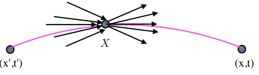
X
(x',t')
(x,t)
Figure 1.Behaviour of the momenta sprays at the midpoint ofhx,t|x0,t0ie.
Better still let us consider a small volume surrounding the midpointX. At this point there is a spray arriving and a spray leaving a volume∆V(X)as shown in Figure1. To see how the local momenta behave at the midpointX, we will use the real part ofS0e(x,x0)defined by
Se(x,x 0) = m
2
(x−x0)2
e . (14)
Then, sinceSe(x,x0) =Se(X,x0) +Se(x,X)atX, we define a quantity
PX(x,x0) =
∂Se(x,x0)
∂X =
∂Se(X,x0)
∂X +
∂Se(x,X)
∂X . (15)
Using the action (14), we find
PX(x,x0) =m
(X−x0)
e −
(x−X)
e
=p0X(x,x0) +pX(x,x0). (16)
What is more important is the relation of equation (16) to equation (10) which is the real part of the weak value of the momentum operator. Thus the mean momentum of a set of Feynman paths at Xis clearly the real part of this weak value. But this weak value is just the Bohm momentum. Thus the Bohm ‘trajectories’ are simply an ensemble of the average of the ensemble of individual Feynman paths.
To see how this unexpected result also emerges from a different perspective, let us consider the process in Figure1which we regard as an image of an ensemble of actual individual quantum processes. We are interested in finding the average behaviour of the momentum,PX, at the pointX. But we have two contributions to consider, one coming from the pointx0and one leaving for the point x. We must determine the distribution of momenta in each spray to produce a result that is consistent with the wave functionψ(X)atX. Feynman suggests [9] that we can think ofψ(X)as ‘information
coming from the past’ andψ∗(X)as ‘potential information appearing in the future’. This suggests that
we can write
lim x0→Xψ(x
0) =Z
φ(p0)eip
0X
dp0 and lim X→xψ
∗(x) =Z
φ∗(p)e−ipXdp.
Theφ(p0)contains information regarding the probability distribution of the incoming momentum
spray, whileφ∗(p)contains information of the probability distribution in the outgoing momentum
spray. These wave functions must be such that in the limite→0 they are consistent with the wave
functionψ(X).
Thus we can define the mean momentum,P(X), at the pointXas
ρ(X)P(X) =
Z Z
Pφ∗(p)e−ipXφ(p0)eip
0X
δ(P−(p0+p)/2)dPdpdp0 (17)
whereρ(X)is the probability density atX. We have added the restrictionδ(P−(p0+p)/2)since
momentum is conserved atX. We can rewrite equation (17) and form
ρ(X)P(X) = 1
2π
Z Z
Pφ∗(p+θ/2)e−iXθφ(p−θ/2)dθdP
or equivalently taking Fourier transforms
ρ(X)P(X) = 1
2π
Z Z
Pψ∗(X−σ/2)e−iPσψ(X+σ/2)dσdP
which means thatP(X)is the conditional expectation value of the momentum weighted by the Wigner function. Equation (17) can be put in the form
ρ(X)P(X) =
1 2i
[(∂x1−∂x2)ψ(x1)ψ(x2)]x1=x2=X. (18)
an equation that appears in the Moyal approach [30], which is based on a different non-commutative algebra. If we evaluate this expression for the wave function written in polar form ψ(x) =
R(x)exp[iS(x)], we findP(X) = ∇S(X)which is identical to the expression for the local (Bohm) momentum used in the Bohm interpretation.
This then confirms the conclusion we reached above, namely, that the set of Bohm ‘trajectories’ is an ensemble of the average ensemble of individual paths. Notice, once again, that this gives a very different picture of the Bohm momentum from the usual one used in Bohmian mechanics [31]. It is not the momentum of a single ‘particle’ passing the pointX, but the meanmomentum flowat the point in question.
constructedstatisticallyfrom an ensemble of individual events. As was shown in Flack and Hiley [26], these flow lines are an average of the momentum flow as described by theweakvalue of the Poynting vector. This agrees with what one would expect from standard quantum electrodynamics, where the notion of a ‘photon trajectory’ has no meaning, but the notion of a ‘momentum flow’ does have meaning.
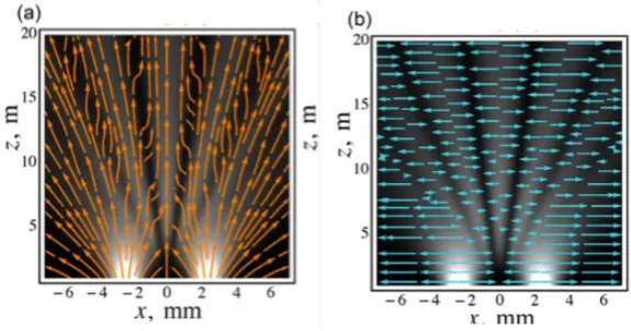
Figure 2.(a) Local field momentum, (b) Localising field momentum.
Bliokh et al. [32] have presented a beautiful illustration showing the results of a two-slit interference experiment. Figure 2(a) shows the real part of the momentum flow lines in the electromagnetic field, while the imaginary component (osmotic) momentum flow lines are shown in Figure2(b). It is then clear that we can regardvB(x,t) = pB(x,t)/mas alocalvelocity, while the osmotic velocityvO(x,t) =pO(x,t)/mcan be regarded as alocalisingvelocity as discussed in Bohm and Hiley [33]. The osmotic velocity behaves in such a way as to maintain the form of the probability distribution.
2.2. Where is the Quantum Potential?
One of the features that many find ‘mysterious’ [34] is the appearance of the ‘quantum potential’ in the Bohm approach. Is there any trace of it in the Feynman paper [9]? To answer this question, we must first refer to de Gosson and Hiley [18] where it is shown that this energy term is absent in quantum processes when taken only toO(∆t=e)so we must consider terms toO(∆t=e2).
Feynman shows that the kinetic energy is ofO(e2)when written in the form K.E = [(xk+1− xk)/e]2, and diverges ase→0. Feynman points out that this quantity is not an observable functional.
But if we define the kinetic energy to be
K.E.0 = m 2
x
k+1−xk
e
xk−xk−1
e
.
This function is finite toO(e)and therefore is an observable functional. Feynman then shows that if
we allow “the mass to change by a small amount tom(1+δ)for a short time, sayearoundtk" we can obtain the relation
m 2
xk+1−xk
e
xk−xk−1
e
= m
2
xk+1−xk
e
2 + h¯
2ie (19)
the extra term arising from the normalising functionA. Thus we must add a ‘correction’ term to the K.E in order for the total energy to be finite toO(e2).
here is not charged so the fluctuations must arise from a different source, but however it arises, it changes the TPA byδ.
Later in the same paper, Feynman shows that any random fluctuation in the phase function will produce the same effect. A random fluctuation at the point xk implies we must replace S(xk+1,tk+1;xk,tk)bySδ(xk+1,tk+1;xk,tk−δ). Thus to the first order inδwe have
hξ|1|ψiS− hξ|1|ψiSδ = iδ
¯
hhξ|Hk|ψiS whereHkis the Hamiltonian functional
Hk=−
∂S(xk+1,tk+1;xk,tk)
∂tk+1
+ h¯
2i(tk+1−tk)
. (20)
Apart from the minus sign, the last term is identical to the last term in equation (19). Thus Feynman required extra energy to appear from somewhere. A more detailed discussion of this feature appears in Feynman and Hibbs [35]. The Bohm approach indicates that some ‘extra’ energy appears in the form of the quantum potential energy at the expense of the kinetic energy. Could it be that the source of the energy is the same?
To explore this possibility, let us use the method explained in section1.3to obtain a more general result for the K.E. The real part of the weak value of the momentum operator squared is obtained from hψ(t)|pˆ2|xi+hx|pˆ2|ψ(t)i/2. Under polar decomposition of the wave function, we find the real part
of the weak value of the kinetic energy is
1 2mhpˆ
2i w = 1
2m
(∇S)2−∇ 2R R
. (21)
With the identification∇S↔m(xk+1−xk)/e, we see that the quantum potential is playing a similar
role as the mass/energy fluctuation in Feynman’s approach. In fact de Broglie’s original suggestion was that the quantum potential could be associated with a change of the rest mass [36].
Notice that the quantum potential appears essentially as a derivative of the osmotic velocity, which in turn is obtained from the imaginary part ofS(x,x0). Any fluctuating term added to the real part ofSe(x,x0)should also be added to the imaginary part. This would also introduce some change in the energy relation shown in equation (20). This interplay between the real components of the complex Se(x,x0)is clearly presented as an average over fluctuations arising from some background. Here we can recall Bohr insisting that the quantum phenomena must include a description of the whole experimental arrangement. More details will be found in Smolin [37] and in Hiley [38].
3. Conclusion
Our explorations of the weak values of the momentum operator [23] have led us to reconsider the basis on which Feynman [9] developed his path integral approach. We have shown that there is an unexpected close connection between the Feynman propagator, the weak values of the momentum and the original Bohm approach [13].
Feynman had already noticed that to prevent the kinetic energy tending to infinity as the time interval between steps tends to zero, it was necessary to introduce a ‘fluctuation’ in the mass/energy of the particle. This extra energy can be thought of as arising in a way similar to the way the quantum potential energy appears as an effect of some background field. Indeed, as we have remarked above, de Broglie [36] had already proposed that the quantum potential could be included in the mass term M = √[m2+ (¯h2/c2)R/R],Rbeing the amplitude of the wave function. Hiley [38] has shown a similar conclusion arises for the Dirac equation.
al.[6] fromPB(x,t)cannot be maintained. Rather the trajectories should be interpreted as a statistical average of the momentum flow of a basic underlying stochastic process.
It is now possible to experimentally explore weak values, perhaps clarifying the nature of this stochastic process. In the case of the electromagnetic field this has already been done by Kocsiset al.[5], but as we have seen the notion of a ‘photon trajectory’ has no meaning. However, the average momentum flow does have meaning [26]. As mentioned above, new experiments using argon and helium atoms are now being carried out at UCL by Morleyet al.[29] and by Monachello, Flack, and Hiley [28]. It is hoped that these future experiments will throw more light on the nature of individual quantum processes.
Acknowledgments: Special thanks to Bob Callaghan, Glen Dennis and Lindon Neil for their helpful discussions. Thanks also to the Franklin Fetzer Foundation for their financial support.
References
1. Landau, L. D.; Lifshitz, E. M.Quantum mechanics: non-relativistic theory. Pergamon Press Oxford 1977. 2. Einstein, A. Albert Einstein: Philosopher-Scientist, Schilpp, A.P., Ed.,Library of the Living Philosophers.
Evanston, Illinois1949; pp. 665-676.
3. Heisenberg, W.Physics and Philosophy: the revolution in modern science. George Allen and Unwin , London, 1958.
4. Jammer, M.The Philosophy of Quantum Mechanics. Wiley, New York 1974.
5. Kocsis, S.; Braverman, B.; Ravets, S.; Stevens, M. J.; Mirin, R. P.; Shalm, L.K.; Steinberg, A. M. Observing the Average Trajectories of Single Photons in a Two-Slit Interferometer.Science,2011,332; 1170-73.
6. Philippidis C.; Dewdney, C. ; Hiley, B. J. Quantum Interference and the Quantum Potential.Nuovo Cimento,
1979,52B; 15-28.
7. Mahler, D. H.; Rozema, L. A.; Fisher, K.; Vermeyden, L.; Resch, K. J.; Braverman, B.; Wiseman,H. M. ; Steinberg, A.M. Measuring Bohm trajectories of entangled photons. InLasers and Electro-Optics (CLEO),2014
Conference on, pp. 1-2. IEEE, 2014.
8. Aharonov, Y.; Albert, D. Z.; Vaidman, L. How the Result of a Measurement of a Component of the Spin of a Spin-1/2 Particle Can Turn Out to be 100.Phys. Rev. Lett.,1988,60; 1351-4.
9. Feynman, R. P. Space-time Approach to Non-Relativistic Quantum Mechanics.Rev. Mod. Phys.,1948,20; 367-387.
10. Schwinger, J. The Theory of Quantised Fields I.Phys. Rev.,1951,82; 914-927.
11. Dirac, P. A. M. On the analogy between Classical and Quantum Mechanics. Rev. Mod. Phys.,1945,17; 195-199.
12. Nelson, E. Derivation of Schrödinger’s Equation from Newtonian Mechanics.Phys. Rev.,1966,150, 1079-1085. 13. Bohm, D. A Suggested Interpretation of the Quantum Theory in Terms of Hidden Variables, I.Phys. Rev.,
1952,85, 166-179; and II.85, 180-193.
14. Dirac, P. A. M.The Principles of Quantum Mechanics. Oxford University Press, Oxford, 1947.
15. Guillemin, V. W. ; Sternberg, S. Symplectic Techniques in Physics. Cambridge University Press, Cambridge 1984.
16. de Gosson, M. ; Hiley, B. J. Imprints of the Quantum World in Classical Mechanics.Found. Phys.,2011,41, 1415-1436.
17. Brown, L. Feynman’s Thesis: A New Approach to Quantum Mechanics. World Scientific Press, Singapore, 2005.
18. de Gosson, M.; Hiley, B. J. Short-Time Quantum Propagator and Bohmian Trajectories.Phys. Lett.,2013,A 377, 3005-3008.
19. Hirschfelder, J. O.; Christoph A. C. ; Palke W. E. Quantum mechanical streamlines I. Square potential barrier.
J. Chem Phys.,1974,61, 5435-55.
20. Hirschfelder, J. O. Quantum Mechanical Equations of Change. I.J.Chem. Phys.,1978,68, 5151-62.
21. Bohm, D. ; Hiley, B. J. Non-locality and Locality in the Stochastic Interpretation of Quantum Mechanics.
Phys. Reports,1989,172, 93-122.
23. Hiley, B. J. Weak Values: Approach through the Clifford and Moyal Algebras.J. Phys.: Conference Series,2012,
361, 012014.
24. Leavens, C. R. Weak Measurements from the point of view of Bohmian Mechanics.Found. Phys.,2005,35, 469-91.
25. Wiseman, H. M. Grounding Bohmian mechanics in weak values and Bayesianism. New J. Phys.,2007,9, 165-77.
26. Flack, R. ; Hiley, B. J. Weak Values of Momentum of the Electromagnetic Field: Average Momentum Flow Lines, Not Photon Trajectories.2016arXiv:1611.06510.
27. Bohm, D.; Hiley, B. J. ; Kaloyerou, P.N. An Ontological Basis for the Quantum Theory: II -A Causal Interpretation of Quantum Fields.Phys. Reports,1987,144, 349-375.
28. Monachello, V.; Flack, R. ; Hiley, B. J. A method for measuring the real part of the weak value of spin using non-zero mass particles.2017arXiv:1701.04808.
29. Morley, J.; Edmunds, P. D.; Barker, P. F. Measuring the weak value of the momentum in a double slit interferometer.J. Phys. Conference series,2016,701, 012030.
30. Moyal, J. E. Quantum Mechanics as a Statistical Theory.Proc. Camb. Phil. Soc.,1949,45, 99-123. 31. Dürr, D. ; Teufel, S.,Bohmian mechanics. Springer Berlin Heidelberg, 2009.
32. Bliokh, K. Y.; Bekshaev, A. Y.; Kofman, A. G. ; Nori, F. Photon trajectories, anomalous velocities and weak measurements: a classical interpretation.New J. Physics,2013,15, 073022.
33. Bohm, D.; Hiley, B. J.The Undivided Universe: an Ontological Interpretation of Quantum Theory. Routledge, London 1993.
34. Feynman, R. P.; Leighton, R. B. ; Sands, M.The Feynman Lectures on PhysicsIII, Sec 21-8. Addison-Wesley, Reading, Mass, 1965.