Crystallographic textures

Crystallographic textures

Vincent Kloseka

CEA, IRAMIS, Laboratoire Léon Brillouin, 91191 Gif-sur-Yvette Cedex, France

Abstract. In material science, crystallographic texture is an important microstructural parameter which directly determines the anisotropy degree of most physical properties of a polycrystalline material at the macro scale. Its characterization is thus of fundamental and applied importance, and should ideally be performed prior to any physical property measurement or modeling. Neutron diffraction is a tool of choice for characterizing crystallographic textures: its main advantages over other existing techniques, and especially over the X-ray diffraction techniques, are due to the low neutron absorption by most elements. The obtained information is representative of a large number of grains, leading to a better accuracy of the statistical description of texture.

1. Introduction

A macroscopic physical property is a relation between a macroscopic stimulus and a macroscopic response [1]. In their general form, such relations are tensorial to account for possible anisotropy, and tensorial field variables have to be considered. For instance, electrical conductivity describes the relation between the current density vector j and the electric (vector) field E by application of a second order tensor, the conductivity tensor . Or elasticity theory establishes the well-known generalized Hooke law, which is a linear relation between the stress1_{and straintensors, which are second order symmetric tensors,} introducing the 4th_{order elastic stiffness tensor C.}

A single crystal being intrinsically an anisotropic (although periodic) arrangement of atoms, most single crystal physical properties are anisotropic, i.e., they are dependent on the crystallographic direction: isotropy is the exception. For instance, the variations of the Young modulus of a Cu single crystal are plotted on Fig. 1 as a function of the crystallographic direction (along which the uniaxial elastic stress is applied and the elastic strain is measured): Cu is stiffer along <111>directions, the Young modulus being almost three times larger than along<100>. Of course, the anisotropy of a single crystal physical property depends on the crystal symmetry (Sect.2), but also on the tensorial nature of the stimulus-response relation: for instance, any property which is described by a 2nd _{order tensor (e.g., the} conductivity, the thermal dilatation, etc.) is nevertheless isotropic if the crystal symmetry is cubic. Crystal symmetries and their influence on single crystal physical properties are the subject of several books: for instance, the preliminary study of “classic” Ref. [2] is highly recommended.

A polycrystal is an aggregate of numerous single crystals more or less randomly orientated. Hence, its macroscopic physical properties should be directly influenced by the

a_{e-mail:[email protected]}

1_{It is unfortunate that standard notation uses the samesymbol for both conductivity and stress tensors.}

Figure 1. Variation of the Young modulus in a Cu crystal as a function of crystal orientation [3]. local and statistical distributions of grains orientations, as well as by the nature of the interactions between adjacent grains.

Crystallographic texture describes the preferential orientations of the crystallites within a polycrystalline sample, or, in other words, the non uniform distribution of crystallographic orientations. It is thus an important microstructural parameter whose representation can be either statistical or local, either qualitative of quantitative. However, in crystallography, defining an orientation is not trivial and depends on the context: are we dealing with the lattice orientation, the crystal orientation (i.e., the orientation of the crystalline motif), the Laue orientation, etc.? Actually, the questions to ask should be: (i) which orientation definition is the most relevant regarding the physical properties of interest? (ii) what are we able to measure, especially by means of neutron diffraction techniques?

In this chapter, we will only deal with the statistical description of the crystallographic texture, since it is the most relevant description regarding (i) the observation scale in neutron diffraction; and (ii) the macroscopic properties of a material.

2. Crystal symmetry and sample symmetry

2.1 Crystal symmetry: Definition of an orientation

Symmetry elements of the macroscopic properties of a crystal are restricted to proper and improper rotation operators. Translation operators have no influence here because the relevant parameter is the direction along which a property is measured: a translation operation does not affect this direction. Rotation (proper and improper) operators make a subgroup of the crystal space group which is called the point group: it is merely obtained from the space group by removing all translations and by moving all rotation axes through the same point. Point groups are therefore the relevant symmetry groups for discussing crystal macroscopic properties: the well-known Neumann’s principle already stated in 1885 that “the symmetry elements of any physical property of a crystal must include the symmetry elements of the point group of the crystal.”

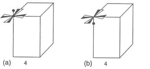
Figure 2. Example of two fictious enantiomorphs with artificial motifs, represented with the same lattice orientation. The crystal system is tetragonal. Crystal orientation (b) can not be obtained from (a) by applying an inversion center: (a) and (b) correspond to two different structures. However (a) and (b) can not be distinguished by means of “classical” diffraction methods since the latter artificially add an inversion center: (a) and (b) belong to the same Laue group (4), and have the same Laue orientation. (Figure reproduced from [1]).

(i.e. implying a center of symmetry which may or not be present in the crystal structure) can be distinguished. This has important consequences for materials which crystallize with a non-centrosymmetric point group, since diffraction artificially adds an inversion center. For instance, two enantiomorphs of the same material with the same lattice orientations but whose crystal orientations are related by a simple inversion have the same Laue orientation, and are impossible to distinguish by “classical” diffraction methods (Fig. 2). Another consequence is that, in the general case, only centrosymmetric physical properties can be analyzed, discussed, predicted or modeled from the single knowledge of the Laue orientation: non-centrosymmetric properties, described by odd-rank tensors (such as electric polarization, piezo-electricity, etc.), can be present in non-centrosymmetric crystals only, and their treatment thus requires the knowledge of the true structure orientation [2,4].

In the following, the term “orientation” will always stand for “Laue orientation”.

2.2 Sample symmetry

In practice, the shape of a polycrystalline material reflects its thermo-mechanical history: e.g., a plate is generally obtained by means of rolling, a wire by drawing, etc. A “sample” symmetry can thus be defined as a statistical symmetry resulting from its elaboration process, and should describe relationships between observed crystallites orientations. As a rule, this sample symmetry reflects the lowest symmetry deformation.

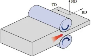
To fix ideas, let us consider for instance a rolling deformation process (Fig.3). It involves a plane strain deformation of the polycrystal, and the resulting sample symmetry should be orthorhombic: if one considers a reference orthogonal frame made of the rolling direction (RD), transverse direction (TD) and normal (to the plate surface) direction (ND), plastic deformation during a rolling process induces grain rotations with mirrors symmetries with respect to (RD, ND), (TD, ND) and (RD, TD) planes. Hence, the sample symmetry is mmm: e.g., from a statistical point of view, as much grains with a lattice direction oriented at an angle from RD are expected as grains with the same lattice direction at− from RD. To provide another example, a torsion process, which involves a simple shear, should lead to a monoclinic sample symmetry.

Figure 3. Rolling deformation process of a thick plate.

property of a polycrystalline sample must include the statistical elements common to its crystallographic texture [1]. The symmetry of a polycrystalline sample is generally reported by using the “crystal symmetry – sample symmetry” doublet notation. For instance, a rolled iron sheet generally exhibits a cubic-orthorhombic symmetry.

Finally, it is important to stress that, in a polycrystal, anisotropy of a physical property results from the anisotropy of this property in the single crystal and the presence of crystallographic texture, simultaneously: an isotropic single crystal property always implies an isotropic polycrystal property (even if the sample is highly textured), and the absence of texture always implies isotropy of macroscopic properties (even for highly anisotropic single crystal properties).

3. Representations of orientations – the orientation

distribution function

3.1 Representations – Euler angles

In crystallographic textures analysis, representing an orientation consists in finding a description of the orientation of the crystallographic axes of a given crystallite, or a group of crystallites, within the polycrystal with respect to the chosen sample coordinate system, and vice-versa. Let us recall that it is always possible to define orthogonal coordinate systems for the crystal and the sample, whatever the crystal and sample symmetries: for instance, considering a general crystal lattice defined by a, b and c unit vectors (and,andlattice angles) the easiest way consists in defining a z vector normal to the (a, b) plane, a y vector parallel to b, and a x vector normal to the resulting (y, z) plane. The same kind of procedure can be applied to obtain an orthogonal (X, Y, Z) sample coordinate system.

There are various ways of describing an orientation. A classic, very simple way of describing an orientation, which is still widely used e.g., in metallurgy due to its compactness and simplicity, consists in making use of the Miller indices of two directions: the first {hkl} indices correspond to the crystal plane whose normal coincides with the “Z” sample frame axis (e.g., the normal direction ND in the case of a rolled sheet), and the second<uvw>

indices correspond to the crystal direction which coincides with the “X” sample frame axis (e.g., the rolling direction RD). This leads to the well-known Miller notation {hkl}<uvw>

for textures components (also called sometimes the metallurgical representation), which still allows the description of textures by means of “ideal orientations”.

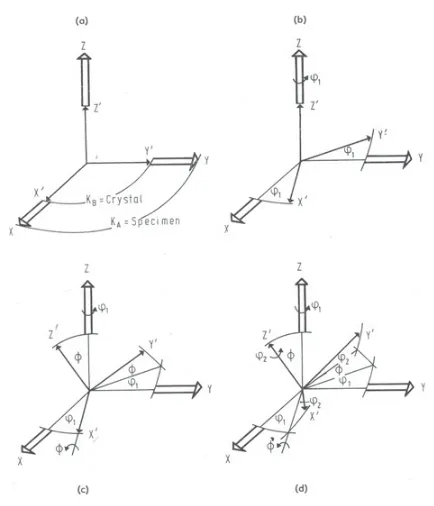
Figure 4. Bunge definition of Euler angles1,,2(see text). Here, the sample axis system is (X, Y, Z) and the rotated crystal axis system is (X’, Y’, Z’) (from [7]).

various conventions (Kocks [5,6], Bunge [7] and Roe [8], mainly). All these conventions are based on the fact that three angles are required to describe a crystal orientation, and hence they all lead to the definition of a three dimensional orientation space (the “Euler space”). Here, only the Bunge convention, which is likely to be the most frequently encountered one, will be detailed.

Bunge convention [7] makes use of the classical definition of Euler angles. To represent the orientation of the crystal axis system (CAS) with respect to the sample axis system (SAS), which is taken as the reference frame, three successive intrinsic rotations are considered, starting with the crystal axes overlapping the sample axes (Fig.4). First, the CAS rotates by 1 about the Z axis. Secondly, the CAS rotates byabout the now rotated x axis. Finally, the CAS rotates by2 about the new z axis. Each of these three elemental rotations can be represented by a rotation matrix, and the CAS orientation can thus be represented by the product of these three elemental rotation matrices. The transformation matrix describing the rotations from the SAS to the CAS, i.e., expressing the crystal lattice unit vectors as a function of the sample unit vectors (active rotation convention) is thus written as:

g=    

cos1cos2−cossin1sin2 −cos1sin2−coscos2cos1 sin1sin cos2sin1+cos1cossin2 cos1coscos2−sin1sin2 −cos1sin

sinsin2 cos2sin cos

   .

(1) In the following, an orientation will be represented by its corresponding g matrix.

Figure 5. Definition of a g orientation.

space) [10]. These specific approaches have advantages and disadvantages over Euler angles approaches for specific applications, but these will not be treated here.

3.2 The orientation distribution function

With the description of orientations by Euler angles, each crystallite c, characterized by its own orientation gc, corresponds to one point whose coordinates are (1,,2)c in the

three-dimensional orientation space. Considering all the crystallites which constitute the polycrystalline aggregate thus allows defining the distribution of points in the orientation space, namely the Orientation Distribution (OD). The OD fully and quantitatively describes the crystallographic texture, which is then taken as a set of discrete orientations. However, it is a global, statistical description, at the scale of the polycrystalline aggregate (or a small part of it), ignoring any possible correlation between a grain orientation and its position within the polycrystal. As a consequence, OD provides no information about the local environment of each grain, which may be another important parameter for property calculations: this kind of description (not treated here) is associated to the definition of “orientation correlation functions”, whose determination requires local, microscopy techniques.

For practical purposes and easy manipulation, OD is generally mathematically described by a continuous function, the Orientation Distribution Functionf(g), which has to be fitted to the data, and defined as:

f(g)dg=dV(g)

V , (2)

i.e., f(g) is the volume fraction of grains characterized by an orientation within a region dg around g orientation. With this definition, the ODF may be assimilated to a probability density, but it is generally normalized so that for a fully randomly oriented material, with no crystallographic texture,f(g)=1∀g, hence:

1 82

f(1,,2) sind1dd2=1 (3)

the orientation space volume being equal to 82_{. The infinitesimal volume element in the} orientation space is thus ₈12sind1dd2.

The ODF allows the quantitative description of the crystallographic texture, namely the calculations of volume fractions of crystallites characterized by a g orientation, with a toleratedg misorientation: such a set of grains is called a texture component. Practically, textures are often described in terms of “ideal orientations”: some which are frequently observed2_{have specific names, such as Cube (corresponding to {100}<010>orientations in}

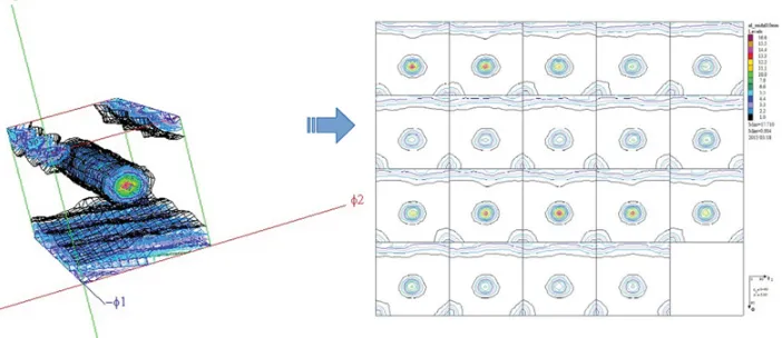
Figure 6. Example of an ODF obtained on a wire-drawn Al alloy, evidencing a {hkl}<111>fiber texture component (parallel to1axis): (left) 3D representation; (right) 2D slices at constant1. Miller notation), Copper ({211}<111>), Goss ({110}<001>), etc. . . for the cubic crystal symmetry. Some textures are also better described as fiber textures (or in term of fiber components) when a rotational symmetry with respect to a sample direction is present: for instance,{hkl}<110>and{111}<uvw>are typical fiber texture components observed in rolled bcc metals, and correspond to rotational symmetries with respect to RD or ND, respectively.

The ODF can be represented in the three-dimensional orientation space by taking the three Euler angles as Cartesian coordinates, with orthogonal axes. From the Bunge’s definition of the Euler angles, this orientation space is periodic in all three axis directions, with a 2 period, thus defining a unit cell (1∈[0, 2],∈[0, 2],2∈[0, 2]). Most of the time, for practical purposes, the ODF is plotted on two dimensional slices of the orientation space, selected at constant1,or2 steps (Fig.6). One dimensional sections may be also used in the case of fiber textures, since in that case the ODF is a function of only two parameters.

Considering the definition of g matrix in (1), OCbeing a crystal symmetry operator and

OSa sample symmetry operator, an equivalent orientation gis obtained by:

g=OCg OS. (4)

These g and gorientations correspond to different points in the orientation space, but these two corresponding rotation matrices represent indistinguishable objects: therefore the ODF must be invariant with respect to the symmetry operations:

f(g)=f(OCg OS)=f(g). (5)

A fundamental zone (or an asymmetric unit) can thus be defined in the orientation space so that each orientation is uniquely described by a single point. Its size depends on the number of crystal and sample symmetry operators: the total volume of orientation space should be divided by the number of symmetry elements. Unfortunately, in the Euler angles representations, this fundamental zone generally has curved boundaries3_{: practically, a} reduced orthogonal orientation space is thus defined from the classical Cartesian, orthogonal

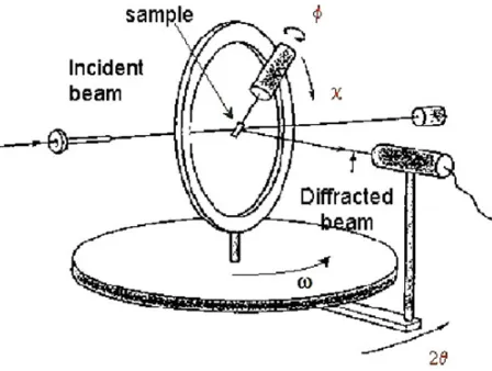
Figure 7. Principle of a 4-circles diffractometer, and definition of rotation angles.

Euler space so that the minimum number of equivalent orientations are contained within appropriate ranges of Euler angles. For instance, for the cubic-orthorhombic symmetry, a reduced, cubic region (1∈[0,/2],∈[0,/2],2 ∈[0,/2]), containing three copies of the actual fundamental zone is used.

Texture index is a widely used parameter globally reflecting the crystallographic texture of a material over the whole orientation space. It is obtained from the ODF knowledge by:

I =

f2(g)dg. (6)

It is equal to 1 for a purely random orientation distribution, and increases with the texture acuteness, i.e., the reinforcement of preferential orientations.

4. Diffraction methods

4.1 Pole figures measurements

The OD (or the ODF) can not be directly determined by an experiment. X-ray and neutron diffraction methods for measuring textures are based on the fact that the diffracted integrated intensity for a specific hkl reflection and for a specific orientation of the diffraction vector (with respect to the sample) is proportional to the diffracting volume, namely the volume of crystallites which are correctly oriented to satisfy the Bragg condition for hkl.

Experimentally, “measuring” a texture by diffraction thus merely consists in measuring the variations of the diffracted intensity with respect to the diffraction vector Qhklorientation.

Using a monochromatic X-ray or neutron source, a classical instrument to reach that purpose is the 4-circles diffractometer (Fig.7): the polycrystalline sample is mounted at the center of an Eulerian cradle, then the diffracted intensity is recorded as a function of the (,) sample orientation, for various hkl reflections, in (, 2) geometry. As a rule, low index hkl reflections are measured in priority since their intensities are usually the highest and they are less subject to peak overlaps. As a result, raw (hkl) diffraction pole figures are obtained, which are projection maps of the diffracted intensities. After experimental corrections and a normalization process, these provide experimental direct pole figures.

Figure 8. Principle of the construction of a 100 pole figure [7].

Figure 9. Example of 111 and 002 experimental pole figures measured on a wire-drawn Al alloy (ODF shown in Fig.6was calculated from these PFs).

(hkl) crystallographic plane. This direction is always taken centrosymmetric: a single crystal Bragg reflection is associated to a pole. Of course, for a given family of equivalent {hkl} crystallographic planes, each crystal constituting the polycrystalline aggregate contributes symmetrically equivalent poles (Fig. 8). Plotting all the poles for all crystallites allows to deduce the pole densityphkl(,) for the polycrystal (Fig.9). Normalization of experimental

pole figures consists in imposing a pole density value equal to 1 for all (,) orientations in the case of a random texture, and in making use of the fact that the total diffracted intensity over a sphere (i.e., over a 4solid angle) is independent of the crystallographic texture, hence:

phkl(,) sindd=4. (7)

As a result, a normalized experimental hkl pole figure is the polar plot ofphkl(,), namely

the volume fractions of the sample for which the (hkl) plane normal has a (,) orientation in the sample coordinate system.

4.2 From pole figures to the orientation distribution function

Basically, a normalized pole figure for {hkl} is obtained by integration of the orientation distribution function along paths corresponding to 2 rotations of crystallites about their corresponding (hkl) poles. This is traduced in the fundamental equation:

phkl(,)=

1 2

₂

0 f

(1,,2)d (8)

wherecorresponds to the rotation angle with respect to the (hkl) diffracting plane normal. It is to note that, excepting special cases such as (00l)-type poles, the integration path is generally not a straight line in the orientation space. A pole figure can thus be considered as a bi-dimensional projection of the (three-dimensional) ODF. Computing any PF when knowing the ODF is a trivial task, but computing the ODF with the single knowledge of few (typically between 2 and 5) PFs is more difficult: it may be compared with the tomography problem of reconstructing a three-dimensional volume from bi-dimensional images, but with an extremely reduced available amount of images!

Two classes of methods are available for computing ODF from PFs: the harmonic methods, and the discrete (or direct) methods. Both are briefly described in the following, as well as their respective advantages and drawbacks.

4.2.1 Harmonic methods [8,11]

The ODF is periodical with respect to the three rotations characterized by1,and2Euler angles, whereas a pole figure is periodical with respect to the two rotations characterized by andangles (in our convention). On the one side, the ODF can thus be expanded in a series of generalized spherical harmonics, which are orthogonal functions similar to the “classical” spherical harmonics functions but considering three rotations instead of two:

f(1,,2)= ∞

l=0 +l

m=−l +l

n=−l

ClmnTlmn(1,,2), (9)

whereCmn

l are the ODF coefficients (to be determined), andTlmnare the generalized spherical

harmonic functions defined by:

Tlmn(1,,2)=eim2Plmn(cos)ein1, (10)

thePlmnbeing the generalized (and normalized) Legendre polynomials.

On the other side, each pole figure can be expanded in a series of spherical harmonic functions:

p(,)=

∞

l=0 +l

m=−l

Qml Ylm(,), (11)

where Qm

l are the corresponding pole figure coefficients, which can be “easily” calculated

from experimental data, andYm

l are the spherical harmonic functions defined by:

Ylm(,)=Plm(cos)eim, (12)

thePlmbeing the Legendre polynomials.

Crystal and sample symmetries induce selection rules on the Cmnl coefficients: some

may cancel, or some relationships may be obtained between them, thus simplifying the expansions. But the relationships between theClmncoefficients can become complicated to

whose formalism makes use of symmetrized spherical harmonic functions which are expressed as linear combinations of theTlmnandYlmfunctions, respectively, so that invariance

with respect to symmetry operations is verified.

As a result from previous considerations and Eq. (8), a set of linear equations relating the PF coefficients and the (unknown) ODF coefficients is obtained. This set can be solved if the number of Cmn

l unknowns is smaller than or equal to the number of equations,

which depends on the number N of available independent experimental PFs: as a result,

N and the crystal symmetry both fix the maximum degree lmax of the expansion (9). For instance, for cubic crystal symmetries, with only two pole figures, theCmn

l coefficients can

be determined up to lmax=22, but for triclinic crystal symmetries, 29 independent pole figures would be required to determine theCmn

l coefficients only up tolmax=14! Practically, the Cmn

l are obtained by minimizing the square deviation between the experimental

and the re-calculated (expanded in SH series) pole figures, imposing phkl(,)≥0

andf(1,,2)≥0 (positivity constraints).

Harmonic methods allow fast computations and low computing memories since each order of the expansion can be computed separately. Moreover, as a result, a compact representation of the ODF is obtained, since only the ODF coefficients need to be known to reconstruct the whole ODF: this allows an easy manipulation in property calculations.

However, as above-mentioned, the required number of PF can become very large (and sometimes unrealistic) for low crystal symmetries. Furthermore, whatever the symmetry degree, the expansion in a series must be practically truncated at a certain order, and this truncation should not drastically affect the results: these methods thus implicitly assume that the ODF should be a smooth function, i.e., that the texture is not too sharp, which may be too restrictive in some cases. Besides, “ghosts” peaks may be obtained in the computed ODF. Indeed, by definition, a pole distribution on a sphere is always centrosymmetric: as a consequence of Friedel’s law, hkl andhklpole figures are always superposed. But spherical harmonic functions (and the generalized harmonic functions) are centrosymmetric whenlis even only, and antisymmetric otherwise. This means that theClmncoefficients with an oddl

can not be determined by “classical” diffraction. Hence the ODF is generally written as the sum of an even part, which can be determined from experimental data, and an odd part which has no effect on PF but, if neglected, may induce artefacts and spurious peaks (named “ghost peaks”) in the ODF. Several methods have been developed to deal with this issue which is especially critical in non-centrosymmetric crystal symmetries [12–16].

4.2.2 Discrete methods

Here, the ODF computation is directly performed in the orientation space. These methods are based on the representation of PFs and ODF by sets of discrete values, obtained by defining regular grids in the projection space (the pole figures) and in the orientation space, respectively. Projection paths relating ODF cells with PFs cells have then to be established. Of course, each PF cell corresponds to the projection of several ODF cells, and the projection lines depend on the crystal and sample symmetries. As a result, the Eq. (8) can be rewritten in its discrete form:

p(hkl)(y)=

1

N N

i=1

f(y⇐gi) (13)

the arrow symbolizing the projection path to the y cell in the pole figure from the N

the projection paths, and the solution is likely not to be unique if not enough experimental pole figures are available.

Various algorithms for implementing discrete methods have been developed during the last decades. For instance, the Vector Method [17] performs direct inversion of the matrix by introducing geometry constraints on the grids. Other methods, such as WIMV [18] or ADC [19] algorithms, first make an initial estimate of the ODF which is used to compute the corresponding initial pole figures. The latter are compared with the experimental pole figures, then correction factors are applied to the ODF to compute new pole figures, and the process is repeated until a good accordance between the calculated and the experimental pole figures is obtained.

Discrete methods have many advantages over harmonic methods. They are generally better suited to sharp textures, but also to low symmetries, since the required amount of pole figures may be reduced. Moreover, most of softwares which implement discrete methods easily allow to impose some positivity and zero-range constraints on the ODF, and also to take into account various symmetries. However, these methods require lots of computing memory, since the matrix relating the orientation space and the pole figures can be very large (although sparse): efficient and optimized programming is thus highly required. Experimental data accuracy is also more critical than with harmonic methods. Besides, the obtained discrete ODF, which consists in a large set of (g,f(g)) doublets, is generally less fit for use in e.g., property calculations than reduced sets of coefficients as obtained by means of harmonic methods. Finally, let us mention that, in some cases, if additional constraints are not introduced, ghosts peaks may also appear in the obtained ODF, due to rank deficiency in Eq. (13).

4.3 Neutron diffraction vs. X-ray diffraction

4.3.1 X-ray diffraction

Figure 10. Left: the two pole figure measurement modes in X-ray diffraction: (a) reflexion; (b) transmission; Right: combination of pole figure regions obtained for each mode (figure reproduced from [21]).

transmission mode (when possible) provides the high region. Then the two sets of data have to be properly merged (Fig.10).

Besides, a diffraction pole figure should plot the diffracted intensity variations due solely to the different volumes of grains in diffraction condition as a function of the sample orientation. The intensity variations due to the different X-ray path lengths within the matter as a function of the sample orientation have thus to be properly corrected. But the X-ray absorption coefficients are large for most elements, and small variations in these path lengths may induce quite large intensity variations. As a consequence, absorption correction is another critical step in the X-ray data treatment.

Rq. It is to note that crystallographic texture measurements can also be performed by means of X-ray synchrotron radiation diffraction. However, it is most of the time difficult to obtain diffraction patterns for numerous sample orientations. Using a bi-dimensional detector, and when the number of available Debye rings is large, it is possible in some specific cases to determine the orientation distribution with a single sample orientation [22]. Taking advantage of the small beam sizes, synchrotron diffraction is better suited to the mapping of orientations at the grain scale, e.g., by means of 3D-XRD [23], or Laue micro-diffraction [24] techniques. Obtained information is then generally far from being statistically representative of the whole sample, and these local measurement techniques are not used to determine orientation distributions.

4.3.2 Neutron diffraction

The main advantage of neutrons over X-rays is their low absorption by most elements [25]. Measurements can thus be performed in transmission mode on massive samples to obtain complete pole figures in a single experiment. The only necessary data correction to be carried out is the background subtraction: absorption correction is generally useless, and there is no defocussing effect. Hence data processing is greatly simplified. Sample volumes of the order of a cm3_{can be characterized, allowing texture analysis over statistically representative} amounts of crystallites, and, as a consequence, errors on the computed ODF are generally significantly lower than with X-ray diffraction: the mean difference between re-calculated and experimental pole figures can be smaller than∼5%, to be compared with∼15% classically obtained from XRD data.

there is generally a quite large tolerance on the sample geometry without having to correct from anisotropic absorption effects: for instance, between two Fe thicknesses of 5 mm and 2 mm, the absorption difference of thermal neutrons is close to 6% only, which practically induces a negligible effect on the measured diffracted intensities. Most samples may thus have cubic-like shapes (much easier to obtain than spheres), or even cylindrical or tubular shapes, or still more irregular shapes. Moreover, no sample surface preparation is required.

As a consequence, neutron diffraction for crystallographic texture analysis is more specifically a tool of choice in the following cases:

• coarse-grained materials (with grain size∼mm3_);

• multiphase materials (especially with anisotropic arrangement of the phases, and resulting anisotropic absorption which may be a strong handicap for X-ray measurements);

• geological materials;

• minority phases characterization (down to volume fractions∼1%);

• use of complex sample environments, such as furnaces, cryostats, mechanical testing machines, etc: a typical application consists in in situ monitoring texture evolutions during thermal treatments;

• low crystal symmetries (since neutron scattering lengths are independent of sin/,

high index reflections may be measured with a higher accuracy than with X-ray diffraction);

• magnetic texture analysis.

4.4 Neutron diffractometers

4.4.1 Continuous sources

On continuous neutron sources, crystallographic texture measurements are generally performed with a monochromatic neutron beam, and the typical dedicated instrument is a 4-circles diffractometer (Fig.7), as previously mentioned in Sect.4.1. The sample is mounted at the center of an Eulerian cradle which allows to impose any orientation of the diffraction vector with respect to the sample coordinate system thanks to the two rotations defined by theandangles.

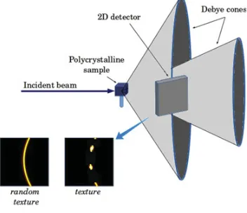
Figure 11. Intercept of a Debye cone by a bi-dimensional flat detector, and example of 2D diffraction images obtained in the case of a random texture (homogeneous Debye rings) and in the case of a textured sample (non homogeneous, “spotted” rings). Each pixel on the detector corresponds to a different Q orientation.

And of course the very low time resolution excludes time-resolved studies from the range of applicability of this technique.

Linear (1D) or bi-dimensional (2D) position sensitive detectors (PSD) can provide interesting alternatives to the single counters4_{. On the one hand, a linear PSD covering a} wide 2range allows the simultaneous recording of a whole diffractogram, i.e., of numerous hkl Bragg peaks for a single sample orientation: by applying appropriate,, rotations to the sample, several hkl pole figures can thus be obtained in a reduced amount of time. This may be especially valuable in the case of in situ, time-resolved experiments, e.g., when characterizing recrystallization or phase transformations at high temperature. Moreover, full diffraction profiles are obtained, and integrated intensities can be used instead of peak intensities, generally leading to a better accuracy. Specific data treatment procedures using Rietveld analysis have been developed to extract texture information from sets of whole diffractograms [26–28].

On the other hand, bi-dimensional detectors can intercept a hkl Debye diffraction cone over a given azimuthal range (Fig. 11): several diffraction vector Qhkl orientations are

thus measured simultaneously, leading to the measurement of numerous (hkl) poles at the same sample orientation. Each pole figure measurements requires less sample rotations, and hence less measurement time. Again, integrated intensities can be extracted. However, data treatment is more complicated than when using a single counter, since it involves image processing, with background, flat-field, and geometric corrections, followed by azimuthal integrations of recorded intensities and a posteriori calculation of the “true” (,) orientation of the diffraction vector. Quite huge amount of data have to be stored and processed, requiring efficient storing and computing solutions.

For instance, 6T1 diffractometer located at LLB (CEA Saclay) [29] uses monochromatic thermal neutrons (=1.159Å) selected by a Cu(111) monochromator at a fixed take-off angle (2m=32◦). An innovative Eulerian cradle with three integrated translations has been

Figure 12. 6T1 diffractometer, at LLB, equipped with its bi-dimensional detector. A small tensile machine is mounted on the Eulerian cradle for in situ mechanical testing.

Figure 13. The 12 positions sample changer of 6T1 diffractometer.

recently mounted, allowing texture mapping or local measuremets in relatively massive samples (Fig.12). Textures can be measured by using either a highly efficient single detector in−2 geometry, or a bi-dimensional detector (200×200 mm2, covering ∼12◦ in 2). A set of four radial collimators allows covering a wide range of divergences and analysis volumes. An original sample changer has been developed to sequentially measure textures of twelve samples without external manual operation (Fig.13). A small tensile machine is also available for in situ measurements.

STRESS-SPEC diffractometer at FRM-II (Munich) [30] is equipped with three different monochromators (Ge(511), bent Si(400) and PG(002)), and the take-off angle can be continuously varied from 2m=35◦to 110◦, allowing to use wavelengths between 1 Å and

2.4 Å: a compromise between resolution and intensity can thus be found for each problem. A full circle Eulerian cradle is available for “light” samples, as well as a 1/4 circle cradle, for heavy samples. A 6-axis robotic arm can also be mounted, which offers more flexibility and can be used as a sample changer (Fig.14). Detection is performed by a bi-dimensional detector (300×300 mm2).

Figure 14. STRESS-SPEC diffractometer, at FRM-II, equipped with its robotic arm.

Figure 15. D1B diffractometer, at ILL, equipped with an Eulerian cradle. The “banana”-type multidetector is inside the green “box”.

but they can also be equipped with an Eulerian cradle to perform crystallographic texture measurements (Fig.15).

4.4.2 Pulsed sources

On pulsed neutron sources, a polychromatic beam is used, and a whole diffractogram

I =f(|Q|) can be measured at a fixed detector position by using the time of flight (TOF) technique5_{. So by taking advantage both of TOF and of several counters or} bi-dimensional detectors located at various angular positions all around the sample, several hkl pole figures can be measured simultaneously with very limited sample rotations. This is highly valuable for performing time-resolved studies, such as recrystallization or phase transformation studies, and/or for measurements involving complex sample environments,

Figure 16. Left: sketch of HIPPO TOF diffractometer, at LANSCE, showing the arrangement of detector tubes in panels arranged on rings of constant diffraction angles. Right: covering of PFs by 3 detector banks for (a) 1 sample orientation and (b) 8 sample orientations [32].

Figure 17. Left: sketch of GEM TOF diffractometer, at ISIS. Right: covering of PFs by 5 detector banks for 2 sample orientations [33].

such as furnaces, pressure cells, etc.. This is also extremely interesting for measuring textures non-destructively in relatively large, precious samples (e.g., archeological objects) which would not fit on an Eulerian cradle. TOF diffractometers are instruments which are by far more complex and expensive than monochromator-based diffractometers, especially due to the huge detector banks and their associated electronics. Besides, TOF data are slightly more difficult to process and analyze than constant wavelength data and data treatment takes naturally high benefit of full-pattern (Rietveld) approaches.

For instance, the detector system of the HIPPO diffractometer at LANSCE [32] consists in 13603_{He detector tubes, arranged in panels, covering a detector area of 4.8 m}2_{and scattering} angles from 10◦to 150◦(Fig.16): only eight sample rotations provide a good coverage of pole figures, with a counting time close to 20 min (Fig.16). GEM diffractometer at ISIS [33] is equipped with 7270 tubes arranged in 6 detector banks, covering a scattering angle range from 1◦to 169◦. For texture measurements, detectors are gathered in 164 groups, each covering ∼10◦×10◦. With this configuration, only 2 or 3 sample rotations are required to get a good coverage of pole figures with collection times of few minutes (cf. Fig.17).

Figure 18. Left: one the 20 prehistoric copper axes which have been analyzed by neutron diffraction (this one has been found in Montecchio, Italy); Right: obtained PFs and inverse PFs evidencing a copper-like texture due to mechanical working along TD followed by thermal recrystallization [36] (mrd = multiple of random distribution).

to the impossibility to fulfill the Bragg law for a given hkl reflection if the wavelength is greater than 2dhkl: when≤2dhkl, diffraction on {hkl} planes can occur, thus contributing to the total absorption cross section, but when≥2dhkl, a sharp increase in the transmitted intensity is generally observed. The height of each step is theoretically proportional to the volume of crystallites having (hkl) planes perpendicular to the incident neutron beam: measuring various hkl Bragg edges for various sample orientations should thus allow to quantitatively analyze the crystallographic texture and its spatial variations. However, only qualitative analysis of texture variations across various materials are reported so far, but improvement of TOF techniques at pulsed sources for neutron imaging may make possible quantitative characterizations in the near future.

5. Examples

5.1 Archaeological metals [36, 37]

Neutron diffraction is an extremely valuable tool for the characterization of materials related to cultural heritage, since the large penetration of neutrons in most materials generally allows to perform measurements on relatively large, massive objects which are mostly precious, without having to cut and take small samples from them, and without specific surface preparation, i.e., non destructively.

Figure 19. Left: the two harquebusier breastplates with the analysis spots indicated. Right: pole figures recorded on GEM diffractometer from three fragments BP1A (top), BP1C (middle) and BP2A (bottom) [37].

annealed and softened (most are partly recrystallized). Authors deduced that, in the Copper age, mechanical working was not used to harden the metal but rather probably to mask surface casting defects and porosity.

Another quite amusing example deals with the investigation of the manufacturing process of harquebusier breastplates [37]. Textures of two breastplates (BP1 and BP2) from different sources, both initially supposed dated round 1600–1650 AD, were measured on GEM diffractometer (Fig. 19). Diffraction showed that both breastplates were made of ferritic steels, with small quantities of carbides and oxides detected in BP1. Pole figures obtained from BP1 are rather irregular, whereas those obtained from BP2 exhibit typical features of the rolling texture of ferritic steel. The armourers of the 16th and 17th century made their objects by hammering iron blooms into thin metal sheets: the random texture observed in BP1 is thus probably due to random stacking of several hammered iron sheets. However, rolling process was unknown in the 17th century! Moreover, relatively large amounts of Mn (0.31 wt.%) were found from chemical analysis of BP2, but such high Mn contents have never been observed in steels elaborated during the 17th century. Authors thus concluded that BP2 must be a replica, possibly from around 1850–1900 and made for use in the Victorian period.

5.2 Deformation and recrystallization textures in cold wire-drawn copper [38]

Static recrystallization of plastically deformed metallic materials can occur during a high temperature annealing, and lead to the emergence of a new microstructure, generally associated with important evolutions of macroscopic mechanical properties. Its experimental and theoretical study thus still remains an important research area. Two main theories are referred to, which are subjects of debates: the “oriented nucleation” theory is based on a preferential nucleation of grains with specific orientations within the deformed matrix, whereas the “oriented growth” theory considers that nuclei in particular crystallographic orientation relationships with the neighboring grains should grow preferentially.

Due to the statistically representative information it provides, neutron diffraction has been widely applied to follow texture evolution during recrystallization. For instance, deformation and recrystallization textures of cold wire-drawn copper were studied in LLB, especially by taking advantage of a special furnace mounted on the cradle of 6T1 diffractometer to perform in situ diffraction measurements [38].

Copper (purity 99.99%) has been hot rolled and cold wire-drawn at several reduction between 51 and 94%, then annealed at 260◦C. Deformation textures exhibit strong a

Figure 20. Inverse pole figure (in wire direction) of wire-drawn copper at 94% reduction: as deformed (left) and recrystallized (right) [38]. (an inverse PF plots a selected sample direction in the CAS, whereas a direct PF plots the Qhkldirection in the SAS).

Figure 21. Reaction avancement factor calculated from measurements of the diffracted intensity at the center of 111 PF, in situ at various temperatures [38].

the deformation. After the thermal treatment at 260◦C, the recrystallization textures are characterized by a dominant <100>fiber, with a weak<111>fiber which disappears at the highest reduction rates while low volume fraction of<112>and<122>fibers develop (Fig.20).

The recrystallization process was then followed in situ by recording the evolution with timeI(t) of the 111 diffracted intensity at (=0◦,=0◦), at constant temperatures. The reaction advancement factorR(t) of the recrystallization process was thus calculated by:

R(t)= I(0)−I(t)

I(0)−I(∞) (14)

The evolution ofR(t) at various temperature for 94% reduction is plotted in Fig.21. Static recrystallization is a thermally activated process, andR(t) variations at different temperatures allowed to compute the activation energy of the recrystallization process as a function of the strain level. An exponential decay of the activation energy with increasing strain could thus be deduced, reaching values close to 45 kJ/mol at reductions≥90%.

5.3 Deformation of beryllium [39]

Figure 22. Measured (top) and simulated (bottom) 00.1 pole figures for the deformation textures of rolled Be at various strain rates (up to 22% compressive strain, in the direction normal to the page). TT: Through Thickness direction [39].

strain rate, Brown et al. [39] used a coupled neutron diffraction and polycrystalline modelling approach.

Be samples with two distinct starting textures (either nearly random obtained by hot pressing or strongly textured obtained by rolling) were deformed in uniaxial compression at various strain rates (covering a wide range from 0.0001/s to 5/s). Initial and deformation textures were measured on HIPPO diffractometer (LANSCE). A multi-scale constitutive model, which accounts for slip and twinning in each grain, as well as twin reorientation, was applied to simulate stress-strain curves and deformation textures as a function of the strain rate, and the latter were confronted to the experimental results. For instance, Fig.22compares the measured and calculated {00.1} deformation pole figures of the rolled (initially textured) Be after in-plane compression. Authors managed to satisfactorily reproduce the observed flow curves as well as the texture evolutions for all mechanical tests with a unique set of parameters. This experiment – modeling confrontation allowed them to compare the rate sensitivities of the different deformation modes. This should lead to a better understanding of the roles played by plastic anisotropy, and by the competitions between various slip systems and twinning in the mechanical properties of hcp metals.

6. Conclusions

Neutron diffraction is a tool of choice for characterizing crystallographic textures. Its main advantages over other existing techniques, and especially over the X-ray diffraction techniques, are essentially due to the low neutron absorption by most elements. Hence, sample preparation and data treatment are generally easy, bulk measurements are feasible, and complex sample environments (e.g., for in situ studies) can be used as well. Relatively low available neutron fluxes (if compared with X-ray sources) are compensated by the utilization of large neutron beams (>mm2_{): the obtained information is thus representative of a large} number of grains, leading to a better accuracy of the statistical description of texture. Neutron diffraction is also especially well suited to the characterization of materials with particular microstructural features, such as coarse grains, multiple phases, minority phases.

References

[1] U.F. Kocks, C.N. Tomé, H.R. Wenk, Texture and Anisotropy - Preferred Orientations in Polycrystals and their Effect on Materials Properties (Cambridge University Press, 1998)

[2] J.F. Nye, Physical Properties of Crystals; their representation by tensors and matrices (Oxford University Press, 1957)

[3] D. Sander, Z. Tian, J. Kirschner, Sensors 8, 4466 (2008)

[4] S. Matthies, G.W. Vinel, K. Helming, Standard Distributions in Texture Analysis - Maps for the Case of Cubic-Orthorhombic Symmetry, Vol. 1 (Berlin: Akademie-Verlag, 1987)

[5] U.F. Kocks, in Eighth Int. Conf. on Textures of Materials, edited by J. Kallend, G. Gottstein (1988), pp. 31–36

[6] H.R. Wenk, U.F. Kocks, Metall. Trans. 18A, 1083 (1987)

[7] H.J. Bunge, Texture Analysis in Materials Science – Mathematical Methods (London: Butterworths, 1982)

[8] R.J. Roe, J. Appl. Phys. 36, 2024 (1965)

[9] O. Rodrigues, J. Mathématiques Pures et Appliquées 5, 380 (1840) [10] A. Morawiec, J. Pospiech, Textures Microstruct. 10, 211 (1989) [11] H.J. Bunge, Z. Metallk. 56, 872 (1965)

[12] H.J. Bunge, C. Esling, J. Phys. Lett. 40, 627 (1979)

[13] C. Esling, H.J. Bunge, J. Muller, J. Phys. Lett. 41, 542 (1980) [14] H.J. Bunge, C. Esling, J. Muller, J. Appl. Crystallogr. 13, 544 (1980) [15] H.J. Bunge, C. Esling, J. Muller, Acta Crystallogr. A37, 889 (1981) [16] H.J. Bunge, C. Esling, Acta Crystallogr. A41, 59 (1985)

[17] D. Ruer, R. Baro, Adv. X-Ray Analysis 20, 187 (1977) [18] S. Matthies, G.W. Vinel, Phys. Stat. Sol. (b) 112, K111 (1982)

[19] K. Pawlik, J. Pospiech, K. Lücke, Textures Microstruct. 14–18, 25 (1991)

[20] B.D. Cullity, Elements of X-Ray Diffraction (2nd Edition) (Addison-Wesley, Reading, 1978)

[21] C. Esling, H.J. Bunge, Techniques de l’Ingénieur TIB476DUO(M3040) (2015) [22] G. Ischia, H.R. Wenk, L. Lutterotti, F. Berberich, J. Appl. Cryst. 38, 377 (2005) [23] D. Juul Jensen, H.F. Poulsen, Mater. Charact. 72, 1 (2012)

[24] J.S. Chung, G.E. Ice, J. Appl. Phys. 86, 5249 (1999)

[25] H. Rauch, W. Waschkowski, in Landolt-Boernstein (Springer, Berlin, 2000), Vol. 16A, Chap. 6

[27] L. Lutterotti, S. Matthies, H.R. Wenk, A.J. Schultz, J.W. Richardson Jr., J. Appl. Phys. 81, 594 (1997)

[28] R.B. Von Dreele, J. Appl. Cryst. 30, 517 (1997)

[29] www-llb.cea.fr/

[30] H.G. Brokmeier, W.M. Gan, C. Randau, M. Völler, J. Rebelo-Kornmeier, M. Hofmann, Nucl. Instrum. Method. Phys. Res. 642, 87 (2011)

[31] www.ill.eu/

[32] S.C. Vogel, C. Hartig, L. Lutterotti, R.B. Von Dreele, H.R. Wenk, D.J. Williams, Adv. X-Ray Analysis 47, 431 (2004)

[33] W. Kockelmann, L.C. Chapon, P.G. Radaelli, Physica B 385–386, 639 (2006) [34] J.R. Santisteban, L. Edwards, V. Stelmukh, Physica B 385–386, 636 (2006)

[35] J.R. Santisteban, M.A. Vicente-Alvarez, P. Vizcaino, A.D. Banchik, S.C. Vogel, A.S. Tremsin, J.V. Vallerga, J.B. McPhate, E. Lehmann, W. Kockelmann, J. Nucl. Mater. 425, 218 (2012)

[36] G. Artioli, Appl. Phys. A 89, 899 (2007)

[37] S. Leever, D. Visser, W. Kockelmann, J. Dik, Physica B 385–386, 542 (2006) [38] P. Gerber, S. Jakani, M.H. Mathon, T. Baudin, Mat. Sci. Forum 495–497, 919 (2005) [39] D.W. Brown, I.J. Beyerlein, T.A. Sisneros, B. Clausen, C.N. Tomé, Int. J. Plast. 29,