B
→
D
∗ν
at non-zero recoil
AlejandroVaquero Avilés-Casco1,,CarletonDeTar1, DapingDu2, AidaEl-Khadra3,4,Andreas Kronfeld4,5,JohnLaiho2, andRuth S.Van de Water4
1Department of Physics and Astronomy, University of Utah, Salt Lake City, Utah, 84112, USA 2Department of Physics, Syracuse University, Syracuse, New York, 13244, USA
3Department of Physics, University of Illinois, Urbana, Illinois, 61801, USA 4Fermi National Accelerator Laboratory, Batavia, Illinois, 60510, USA
5Institute for Advanced Study, Technische Universität München, 85748 Garching, Germany
Abstract. We present preliminary results from our analysis of the form factors for the
B→ D∗νdecay at non-zero recoil. Our analysis includes 15 MILC asqtad ensembles
withNf =2+1 flavors of sea quarks and lattice spacings ranging froma≈0.15 fm down
to 0.045 fm. The valence light quarks employ the asqtad action, whereas the heavy quarks are treated using the Fermilab action. We conclude with a discussion of future plans and phenomenological implications. When combined with experimental measurements of the decay rate, our calculation will enable a determination of the CKM matrix element|Vcb|.
1 Introduction
Although the Standard Model (SM) is widely regarded as a very successful theory, its description of nature is not fully satisfactory, and it is believed to be incomplete. This fact has set a large part of the scientific community in the search for physics Beyond the Standard Model (BSM). One of the most promising places to look for new physics is the flavor sector of the SM. In particular, the unitarity triangle and the CKM matrix elements [1,2] have been object of extensive research [3], as newer methods and algorithms improved the precision of the measurements. The latest experimental averages [4,5] reveal a tension of about 3σ between the inclusive and exclusive determinations of
|Vcb|, and it is of foremost importance to investigate the origins of this tension.
One way to obtain|Vcb|is from the decay rate of B → D∗ν. Experimental measurements of this decay rate are precise for large momenta, but noisy at low recoil, due to a supression of the phase space [4]. The lattice approach, on the other hand, excels at low recoil, where it becomes more precise. Forthcoming experiments at LHCb [6] and Belle-II [7], are expected to reduce the experimental uncertainties, so improved lattice calculations are needed to maximize their impact on |Vcb|determinations. In this work we present first, preliminary results of our lattice QCD calculation of the form factors for theB→D∗νprocess at non-zero recoil.
2 Form factor definitions
TheB→D∗νdecay is mediated by aV−Aweak current. The matrix elements can be decomposed in the following way:
D∗(pD∗, ν)| VµB¯(pB) 2√MBMD∗
=1 2ν∗ε
µν ρσv
ρ
BvσD∗hV(w), (1)
D∗(pD∗,
ν)| AµB¯(pB)
2√MBMD∗
= i 2ν∗
gµν(1+w)hA1(w)−vνBvµBhA2(w)+vµD∗hA3(w), (2)
whereVµandAµare the vector and axial, continuum, electroweak currents, respectively. The 4-vectorsvµX (X = B,D∗) are the 4-velocities, defined as vXµ = pµX/MX,w = vB·vD∗ is the recoil
parameter, theνis the polarization of theD∗final state and thehk(w) (k=V,A1,2,3) are the different form factors that contribute to the decay rate.
The differential decay rate can be expressed as
dΓ
dw = G2
FM5B
4π3 r3(1−r)2(w2−1)
1
2|ηEW|2|Vcb|2χ(w)|F(w)|2, (3)
withr = MD∗/MB, the ratio of the meson rest masses andηEW, the electroweak correction factor
for NLO box diagrams. The kinematic factor √w2−1 is what makes experimental measurements so difficult at low recoil. The functionsχ(w) andF(w) are standard, motivated by the heavy-quark limit:
χ(w)=(1+w)2λ(w) with λ(w)= 1+w4+w1t2(w)
12 , t2(w)=
1−2wr+r2
(1−r)2 , (4)
F(w)=hA1(w)
H2
0(w)+H2+(w)+H2−(w)
λ(w) , (5)
where
XV(w)=
w−1
w+1
hV(w)
hA1(w), (6) X2(w)=(w−1)
hA2(w)
hA1(w), (7)
X3(w)=(w−1)hA1hA3((ww)), (8) H0(w)=w−r−X13(w)−rX2(w)
−r , (9)
H±(w)=t(w) (1∓XV(w)), (10) The calculation ofF(w) will allow us to determine |Vcb| from experimental measurements of the differential decay rate.
3 Simulation details
For this analysis we use the same set of ensembles as in the zero recoil publication [9]. These are 15 different MILC asqtad ensembles withNf =2+1 flavors of sea quarks [10]. The valence light quarks are simulated with the asqtad action [11], whereas the heavy quarks use the clover action with the Fermilab interpretation [12]. The calculations on these ensembles are performed atp2 = 0,2Lπ2,4Lπ2 in lattice units, with L the spatial size of the lattice. We distinguish two different
2 Form factor definitions
TheB→D∗νdecay is mediated by aV−Aweak current. The matrix elements can be decomposed
in the following way:
D∗(pD∗, ν)| VµB¯(pB) 2√MBMD∗
=1
2ν∗ε µν
ρσv ρ
BvσD∗hV(w), (1)
D∗(pD∗, ν)| AµB¯(pB) 2√MBMD∗
= i
2ν∗
gµν(1+w)hA1(w)−v
ν B
vµBhA2(w)+v
µ D∗hA3(w)
, (2)
whereVµandAµ are the vector and axial, continuum, electroweak currents, respectively. The
4-vectorsvµX (X = B,D∗) are the 4-velocities, defined as vµX = pµX/MX, w = vB·vD∗ is the recoil parameter, theνis the polarization of theD∗final state and thehk(w) (k=V,A1,2,3) are the different
form factors that contribute to the decay rate. The differential decay rate can be expressed as
dΓ
dw =
G2
FM5B
4π3 r3(1−r)2(w2−1)
1
2|ηEW|2|Vcb|2χ(w)|F(w)|2, (3)
withr = MD∗/MB, the ratio of the meson rest masses and ηEW, the electroweak correction factor
for NLO box diagrams. The kinematic factor √w2−1 is what makes experimental measurements so
difficult at low recoil. The functionsχ(w) andF(w) are standard, motivated by the heavy-quark limit:
χ(w)=(1+w)2λ(w) with λ(w)= 1+w4+w1t2(w)
12 , t2(w)=
1−2wr+r2
(1−r)2 , (4)
F(w)=hA1(w)
H2
0(w)+H2+(w)+H2−(w)
λ(w) , (5)
where
XV(w)=
w−1
w+1
hV(w) hA1(w)
, (6) X2(w)=(w−1)hA2(w)
hA1(w)
, (7)
X3(w)=(w−1)hhA3(w)
A1(w)
, (8) H0(w)=w−r−X13(w)−rX2(w)
−r , (9)
H±(w)=t(w) (1∓XV(w)), (10)
The calculation ofF(w) will allow us to determine |Vcb|from experimental measurements of the differential decay rate.
3 Simulation details
For this analysis we use the same set of ensembles as in the zero recoil publication [9]. These are 15 different MILC asqtad ensembles withNf =2+1 flavors of sea quarks [10]. The valence light
quarks are simulated with the asqtad action [11], whereas the heavy quarks use the clover action
with the Fermilab interpretation [12]. The calculations on these ensembles are performed atp2 =
0,2Lπ2,4Lπ2 in lattice units, with L the spatial size of the lattice. We distinguish two different
cases: momentum perpendicular to theD∗polarization and an average over parallel and perpendicular
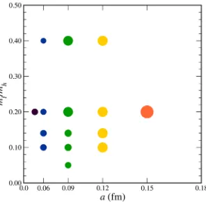
directions. Fig.1shows the size of the ensemble as a function of the lattice spacing and the quark masses. For further details we refer to tables I and II of [9].
Figure 1: List of available ensembles. The area of the circle is proportional to the statistics.
4 Calculation of correlation functions
4.1 Two-point functions and calculation of rest masses and excited states
The 2-point functions give us information about the energy levels of the states, as well as the overlap factorsZ. In this work, the definitions and notation of the 2-point functions follow ref. [13]. We fit 2-point functions for the ¯Band theD∗meson with smeared (1S) and point (d) sources at source and
sink, giving rise to four possible combinations per ensemble and momentum: (1S,1S), (d,d), (1S,d)
and (d,1S), where we combined the latter two into a symmetric average.
For our analysis, we perform the joint fit of the three 2-point functions with different smearings
at the same time on each ensemble. At non-zero momentum (D∗), we also distinguished between
momentum parallel or perpendicular with respect to the meson polarization. Therefore at non-zero momentum our simultaneous fits involve six 2-point functions. We use Bayesian constraints with loosely constrained priors. The main function of the priors here was to prevent the fitter from arriving at absurd values. The prior errors were large enough so small variations in their values didn’t change the final results. The correlation matrix for the fitter was obtained using the jackknife method.
We vary the number of states in our fit function: 1+1, 2+2 and 3+3, where the first figure is
the number of standard states, and the second gives the number of oscillating states. We choose the 2+2 fits, which balance reasonablepvalues results with low errors, and are consistent with the results
coming from the 3+3 fits. The initial time of the fit is chosen after reaching a plateau in the value of
the meson mass, and it is adjusted to be similar in physical units for all the ensembles. The final time is taken to ensure the resultingpvalue is reasonable, i.e., we check that thepvalues follow a uniform distribution.
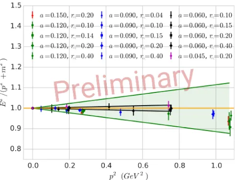
As a consistency check, we test the continuum dispersion relation E2 = p2 +m2 by plotting
E2/(p2+m2) vsp2(fig.2). Discretization effects with large masses (in lattice units) could cause this
quantity to deviate from∼1. Nonetheless, we clearly see an improvement as the lattice spacing is reduced.
4.2 Three-point function ratios and general considerations
We extract the matrix elements from ratios of 3-point correlation functions. To this end, we use the same setup and notation as in [9,13]. We construct the non-zero momentum correlation functions as
CB→D∗
Figure 2: Dispersion relation for theD∗meson, all ensembles. The legend gives the lattice spacingaand the ratio between the light and the strange quark masses, called hererm. The cones represent the expected discretization effects for the green and the black points. Deviations fromE2/(p2+m2) are observed only for the coarsest ensembles at high momenta, and even in the
worst case they are well within the expected discretization errors, of orderOαs(ap)2.
whereOD∗(p,0) andOB(0,T) are interpolating operators with the quantum numbers of theD∗and the
Bmesons, respectively, with 3-momentumpand0, andJis a vector or axial current. Then we can
relate the correlation functions to the matrix elements using CB→D∗
J (p,t,T)=
ZD∗(p)ZB(0)e−ED∗te−MB(T−t)
D∗(p)JB(0)+. . . (12)
TheZX factors are the overlap factors obtained from the 2-point functions of the mesonX, and the exponentials decay with the energy of the constructed states. The missing extra-terms refer to higher excited states, which are suppressed at large values oftandT −t, as well as extra, oscillatory terms, whose contribution is proportional to (−1)tand (−1)T−t. Regarding renormalization and matching, we follow references [9,13], but at the time of the conference the perturbativeρfactors were not available yet.
In our calculations, the parent meson is always at rest andBpropagates from timeT. The daugther meson propagates from time 0, and both of them are tied together at the current insertion pointt. We fix the sink and move the insertion in the range [0,T], expecting the excited states in (12) to die as we
move far from the extremes. The different source-sink separations used in this analysis are listed in
table IV of [9].
From (12) we construct ratios of 3-point functions that remove as manyZfactors and exponentials as possible from the rhs of (12). In order to suppress the effect of the oscillatory terms coming from
the 3-point functions, we use the following weighted average [8]
¯
R(t,T)=1
2R(t,T)+ 1
4R(t,T +1)+ 1
4R(t+1,T+1), (13)
whereRis the ratio to be analyzed,T is the sink time and ¯Ris the weighted average we use for the analysis. This average ensures that the errors introduced by oscillating states are negligible compared with other errors. As a general ansatz to fit the ratios, we use the following function:
Figure 2: Dispersion relation for theD∗meson, all ensembles. The legend gives the lattice spacingaand the ratio between the light and the strange quark masses, called hererm. The cones represent the expected discretization effects for the green and the black points. Deviations fromE2/(p2+m2) are observed only for the coarsest ensembles at high momenta, and even in the
worst case they are well within the expected discretization errors, of orderOαs(ap)2.
whereOD∗(p,0) andOB(0,T) are interpolating operators with the quantum numbers of theD∗and the
Bmesons, respectively, with 3-momentumpand0, andJis a vector or axial current. Then we can
relate the correlation functions to the matrix elements using CB→D∗
J (p,t,T)=
ZD∗(p)ZB(0)e−ED∗te−MB(T−t)
D∗(p)JB(0)+. . . (12)
TheZX factors are the overlap factors obtained from the 2-point functions of the mesonX, and the exponentials decay with the energy of the constructed states. The missing extra-terms refer to higher excited states, which are suppressed at large values oftandT−t, as well as extra, oscillatory terms, whose contribution is proportional to (−1)tand (−1)T−t. Regarding renormalization and matching, we follow references [9,13], but at the time of the conference the perturbativeρfactors were not available yet.
In our calculations, the parent meson is always at rest andBpropagates from timeT. The daugther meson propagates from time 0, and both of them are tied together at the current insertion pointt. We fix the sink and move the insertion in the range [0,T], expecting the excited states in (12) to die as we
move far from the extremes. The different source-sink separations used in this analysis are listed in
table IV of [9].
From (12) we construct ratios of 3-point functions that remove as manyZfactors and exponentials as possible from the rhs of (12). In order to suppress the effect of the oscillatory terms coming from
the 3-point functions, we use the following weighted average [8]
¯
R(t,T)=1
2R(t,T)+ 1
4R(t,T +1)+ 1
4R(t+1,T+1), (13)
whereRis the ratio to be analyzed,T is the sink time and ¯Ris the weighted average we use for the analysis. This average ensures that the errors introduced by oscillating states are negligible compared with other errors. As a general ansatz to fit the ratios, we use the following function:
r(t)=R1+Ae−∆EM0t+Be−∆EMT(T−t), (14)
whereRis the ratio of matrix elements we want to extract,T is the sink time,∆EM0and∆EMT are the
differences between the energies of the first excited and the ground state for the mesons living att=0
andt=T respectively, taken from the 2-point fits, andAandBare fit parameters.
In our analysis we use constrained fits with priors. Whenever the parameters are largely unknown or known with poor precision, a loose prior is set just to guide the fitter. In constrast, whenever the parameters involve quantities obtained in previous fits, the priors are set to the fit outcome and are counted as data points. To remove autocorrelations in our data, we compute the covariance matrix given to the fitter after processing the data with jackknife.
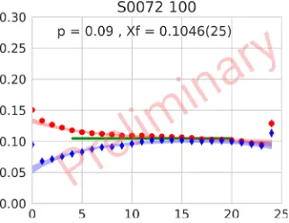
Finally, the parent meson is always smeared using Richardson smearing, but the daughter meson can be smeared or not. This fact gives rise to several versions of each ratio, and following the same technique as in the 2-point function analysis, we perform a joint fit of all the available data to obtain the final results. As an example, we show in fig.3one of the fits we use to estimate the recoil parameter.
Figure 3: Sample ratio fit for a 3-point function ratio,xfin this case. The blue points show the data with a smeared interpolating
operator, whereas the red points represent a point interpolating operator. The green horizontal bar represents the result forRin (14). In this particular case, we forceB=0 because theBsmearing suppresses all the excited states coming from the sink.
5 Form factors from lattice matrix elements
In order to extract the matrix elements from the lattice, we consider several ratios that reduce the errors in the determination of the form factors.
5.1 Recoil parameter
Considering the ¯Bmeson at rest, one can compute the recoil parameter as
w(p)= 1 +x2f(p)
1−x2
f(p)
, (15) xf(p)= D
∗(p)|V|D∗(0)
D∗(p)|V4|D∗(0), (16)
5.2 Axial form factors
5.2.1 Axial double ratioRA1
AlthoughRA1is directly obtained fromD∗(p
⊥)A1B(0)
, it is advantageous to use a ratio,
RA1(p)=
D∗(p
⊥)A1B¯(0)
D∗(0)A1B¯(0) . (17)
Eq. (17) has an important drawback: when expressed as a ratio of 3-point functions, exponentials depending on time are not cancelled for the daughter meson. Hence, we need to add an energy-dependent correction factor before we can fit the ratio on the lattice. In the zero momentum case a double ratio was used to get rid of the exponential and some overlap factors, reducing the errors and improving the quality of the fit [8,9]. Here we can do the same,
RA1(p)2=
D∗(p⊥)A1B(0) B(0)A1D∗(p⊥)
D∗(0)V4B(0) B(0)V4D∗(0) . (18)
From this quantity we can directly extracthA1(w)=2/(1+w)RA1. As we don’t have any measurements
for the matrix elementB(0)A1D∗(p⊥)
, we use time reversalT to reconstruct it from known data,
CD∗→B
(p⊥,t,T)−−→T CB→D∗
A1 (p⊥,T −t,T). (19)
Our preliminary results forhA1(w), computed from eq. (18) is shown in the right pane of fig.4.
5.2.2 RatiosR0andR1
The quantitiesR0andR1
R0(p)=
D∗(p
)A4B(0)
D∗(p⊥)A1B(0), (20) R1(p)=
D∗(p
)A1B(0)
D∗(p⊥)A1B(0), (21) encode the behavior ofhA2(w) andhA3(w) as
R0= √
w2−1(1−hA2+whA3)
(1+w)hA1 , (22) R1=w−
(w2−1)hA3
(1+w)hA1 . (23)
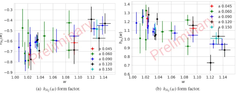
Preliminary results forhA2(w) andhA3(w) are reported in fig.5.
5.3 Vector form factor
The previously defined quantityXV(w) can be measured as the following ratio of matrix elements:
hV = √RA1
w−1XV (24) XV(p)=
D∗(p
⊥)V1B(0)
5.2 Axial form factors
5.2.1 Axial double ratioRA1
AlthoughRA1is directly obtained from
D∗(p
⊥)A1B(0)
, it is advantageous to use a ratio,
RA1(p)=
D∗(p
⊥)A1B¯(0)
D∗(0)A1B¯(0) . (17)
Eq. (17) has an important drawback: when expressed as a ratio of 3-point functions, exponentials depending on time are not cancelled for the daughter meson. Hence, we need to add an energy-dependent correction factor before we can fit the ratio on the lattice. In the zero momentum case a double ratio was used to get rid of the exponential and some overlap factors, reducing the errors and improving the quality of the fit [8,9]. Here we can do the same,
RA1(p)
2 =
D∗(p⊥)A1B(0) B(0)A1D∗(p⊥)
D∗(0)V4B(0) B(0)V4D∗(0) . (18)
From this quantity we can directly extracthA1(w)=2/(1+w)RA1. As we don’t have any measurements
for the matrix elementB(0)A1D∗(p⊥)
, we use time reversalT to reconstruct it from known data,
CD∗→B
(p⊥,t,T)−−→T CAB1→D∗(p⊥,T −t,T). (19)
Our preliminary results forhA1(w), computed from eq. (18) is shown in the right pane of fig.4.
5.2.2 RatiosR0andR1
The quantitiesR0andR1
R0(p)=
D∗(p
)A4B(0)
D∗(p⊥)A1B(0), (20) R1(p)=
D∗(p
)A1B(0)
D∗(p⊥)A1B(0), (21)
encode the behavior ofhA2(w) andhA3(w) as
R0 =
√
w2−1(1−hA2+whA3)
(1+w)hA1
, (22) R1=w−(w
2−1)h
A3
(1+w)hA1
. (23)
Preliminary results forhA2(w) andhA3(w) are reported in fig.5.
5.3 Vector form factor
The previously defined quantityXV(w) can be measured as the following ratio of matrix elements:
hV = √RA1
w−1XV (24) XV(p)=
D∗(p
⊥)V1B(0)
D∗(p⊥)A1B(0). (25)
When this ratio is expressed in terms of lattice 3-point correlation functions, all the exponentials and overlap factors are cancelled, and the result yields directly the quotient of form factors we are looking for. Our preliminary result forhV(w) is shown in the left pane of fig.4.
(a)hV(w) form factor. (b)hA1(w) form factor.
Figure 4: Preliminary results forhV(w) andhA1(w) fromXVand the double ratioRA1. The contribution ofhV(w) toF(w) is suppressed due to kinematic factors, and the final result is clearly dominated byhA1(w).
(a)hA2(w) form factor. (b)hA3(w) form factor.
Figure 5: Preliminary results forhA2(w) andhA3(w) fromR0andR1. We expect to reduce the errors in these form factors when we refine the analysis. However, the contribution ofhA2(w) andhA3(w) toF(w) is highly suppressed by kinematic factors at low recoil. Therefore the final total error is dominated by the errors coming fromhA1(w).
5.4 Results for the form factors as a function of the recoil parameter
In figs.4,5we show the preliminary results for the axial and vector form factors, with statistical errors only, without rho factors, and before taking the chiral-continuum extrapolation. It is important to notice that near zero recoil (for smallw−1), F(w) is dominated byhA1, because the contributions
fromhV,hA2, andhA3are suppressed by kinematic factors (see eqs. (7), (8) and (6)).
6 Summary and future work
to the correlation functions, after which we plan to study the chiral-continuum extrapolations, use the
z-expansion to parametrize the shape, and construct a complete, systematic error budget.
7 Acknowledgements
Computations for this work were carried out with resources provided by the USQCD Collaboration, the National Energy Research Scientific Computing Center and the Argonne Leadership Computing Facility, which are funded by the Office of Science of the U.S. Department of Energy; and with resources provided by the National Institute
for Computational Science and the Texas Advanced Computing Center, which are funded through the National Science Foundation’s Teragrid/XSEDE Program. This work was supported in part by the U.S. Department of
Energy under grants No. DE-FC02-06ER41446 (C.D.) and No. DE-SC0015655 (A.X.K.), by the U.S. National Science Foundation under grants PHY10-67881 and PHY14-17805 (J.L.), PHY14-14614 (C.D., A.V.); by the Fermilab Distinguished Scholars program (A.X.K.); by the German Excellence Initiative and the European Union Seventh Framework Program under grant agreement No. 291763 as well as the European Union’s Marie Curie COFUND program (A.S.K.).
Fermilab is operated by Fermi Research Alliance, LLC, under Contract No. DE-AC02-07CH11359 with the United States Department of Energy, Office of Science, Office of High Energy Physics. The publisher, by
accepting the article for publication, acknowledges that the United States Government retains a non-exclusive, paid-up, irrevocable, world-wide license to publish or reproduce the published form of this manuscript, or allow others to do so, for United States Government purposes.
References
[1] N. Cabibbo, Phys. Rev. Lett.10, 531 (1963), [,648(1963)] [2] M. Kobayashi, T. Maskawa, Prog. Theor. Phys.49, 652 (1973) [3] M. Antonelli et al., Phys. Rept.494, 197 (2010),0907.5386
[4] C. Patrignani et al. (Particle Data Group), Chin. Phys.C40, 100001 (2016) [5] Y. Amhis et al. (2016),1612.07233
[6] R. Aaij, B. Adeva, M. Adinolfi, Z. Ajaltouni, S. Akar, J. Albrecht, F. Alessio, M. Alexander, S. Ali, G. Alkhazov et al. (LHCb Collaboration), Tech. Rep. CERN-LHCC-2017-003, CERN,
Geneva (2017),http://cds.cern.ch/record/2244311
[7] T. Abe et al. (Belle-II), Tech. rep., KEK (2010),1011.0352,http://arxiv.org/pdf/1011. 0352v1
[8] C. Bernard et al., Phys. Rev.D79, 014506 (2009),0808.2519
[9] J.A. Bailey et al. (Fermilab Lattice, MILC), Phys. Rev.D89, 114504 (2014),1403.0635
[10] A. Bazavov et al. (MILC), Rev. Mod. Phys.82, 1349 (2010),0903.3598
[11] G.P. Lepage, Phys. Rev.D59, 074502 (1999),hep-lat/9809157
[12] A.X. El-Khadra, A.S. Kronfeld, P.B. Mackenzie, Phys. Rev. D55, 3933 (1997),
hep-lat/9604004