The trade-off between the controller effort and

Article

1

The trade-off between the controller effort and

2

control quality on example of an electro-pneumatic

3

final control element

4

Michał Bartyś 1,_{*, Bartłomiej Hryniewicki} 2

5

1 _{Warsaw University of Technology, Institute of Automatic Control and Robotics; PL 02-525 Warsaw,}

6

św. A. Boboli 8, bartys@mchtr.pw.edu.pl

7

2 _{Warsaw University of Technology, Institute of Automatic Control and Robotics; PL 02-525 Warsaw,}

8

św. A. Boboli 8, 258971@pw.edu.pl

9

* Correspondence: bartys@mchtr.pw.edu.pl; Tel.: +48-501-697-545

10

11

Featured Application: process control engineering practice. This paper shows that by the proper

12

selection of the structure and parameters of the internal controller of the final control element, one

13

can achieve two seemingly contradictory outcomes. On the one hand, better quality control, while

14

on the other, simultaneous reduction of the controller effort, which in turn leads to a significant

15

extension of the mean-time-between-failures of the final control element. This has a pertinent

16

impact on functional safety and economy of the process.

17

Abstract: For many years, the programmable positioners have been widely applied in structures of

18

modern electro-pneumatic final control elements. The positioner consists of an electro-pneumatic

19

transducer, embedded controller and measuring instrumentation. Electro-pneumatic transducers

20

that are used in positioners are characterized by a relatively short mean time-to-failure. The

21

practical and economical method of a reasonable prolongation of this time is proposed in this

22

paper. It is principally based on assessment and minimizing the effort of the embedded controller.

23

For this purpose, were introduced: the control value variability, mean-time and the cumulative

24

controller's effort. The diminishing of controller effort has significant practical repercussions,

25

because it reduces the intensity of mechanical wear of the final control element components. On the

26

other hand, the reduction of the cumulative effort is important in the context of process economy

27

due to limitation of the consumption of energy of compressed air supplying the final control

28

element. Therefore, the minimization of introduced effort factors has an impact on increasing the

29

functional safety and economics of the controlled process. As a result of the performed simulations,

30

the recommendations regarding the selection of the structure and tuning of positioner controller

31

were elaborated. The simulations were performed in the Matlab-Simulink environment with the

32

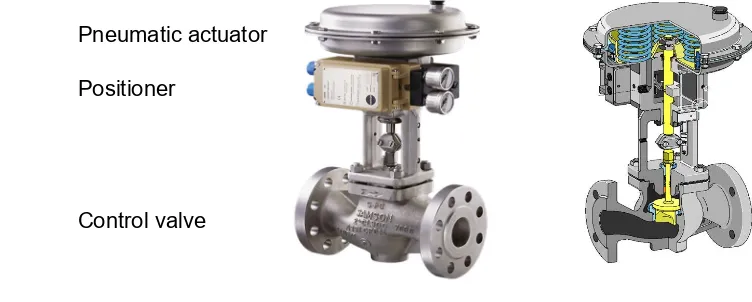
use of the liquid level control system in which a phenomenological model of a final control element

33

was deployed. It has been proven that under appropriate conditions, it is possible to extend

34

significantly the lifetime of the final control element and simultaneously enhance the control

35

quality factors.

36

Keywords: final control element; electro-pneumatic transducer, controller effort, control quality

37

factors, wear, mean-time-between-failures

38

39

1. Introduction

40

In the structures of the closed loop industrial automation systems, we can generally distinguish:

41

controlled systems, controllers, measuring instrumentation and final control elements [1-3]. The

42

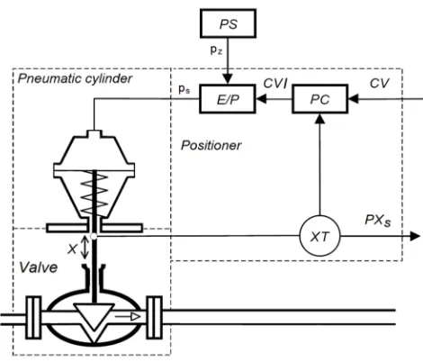
general structure of a single-loop control system is depicted in Figure 1. The final control elements

43

are physical units directly affecting the streams of energy and materials. In the structure of a control

44

system, they simply play the role of adapters between controllers and controlled systems.

45

In fact, the final control elements are acting as energy or power converters that convert the

46

low-energy or informative control value (CV) into a high-energy driving signal (CVa). Clearly, due to

47

the principle of energy conservation, the final control elements require an additional auxiliary power

48

supply source.

49

50

51

52

53

54

55

56

Figure 1. Block diagram of the structure of the closed loop automatic control system. Notion: SP –

57

setpoint; PVs – measured value of process variable; e - control error; CV – controller output; CVa –

58

final control element actuator output; PV- process variable.

59

The main interest of this paper is focused on the certain class of final control elements in which

60

the compressed air is used as an auxiliary energy supply source. These elements are commonly used

61

in automatic control systems used in the following industries: power, chemical, petrochemical,

62

pharmaceutical and food.

63

A typical electro-pneumatic final control element consists of a pneumatic actuator with linear or

64

rotational movement of its rod, a positioner and a control valve (Figure 2). By adjusting the position

65

of the valve plug attached to the end of actuator’s rod towards the valve seat, it is possible to control

66

the flow rate of a medium passing through the valve.

67

The primary goal of the positioner is to follow-up the CV. In order to do it, the positioner has to

68

control the pressure of the pneumatic actuator in such a way that the position of the valve plug will

69

depend exclusively on CV and will suppress the influence of the disturbances such as: changes of

70

operating temperature, supply pressure fluctuations, changes in the static and dynamic load of the

71

actuator’s rod, friction and the evolution of friction forces.

72

73

74

75

76

77

78

79

Figure 2. An example of an electro-pneumatic final control element and cross-section of its

80

mechanical construction [4,5].

81

The final static and dynamic properties of the actuator are shaped by the positioner. In fact, the

82

positioner is a specialized, autonomous control system of the rod position. The simplified block

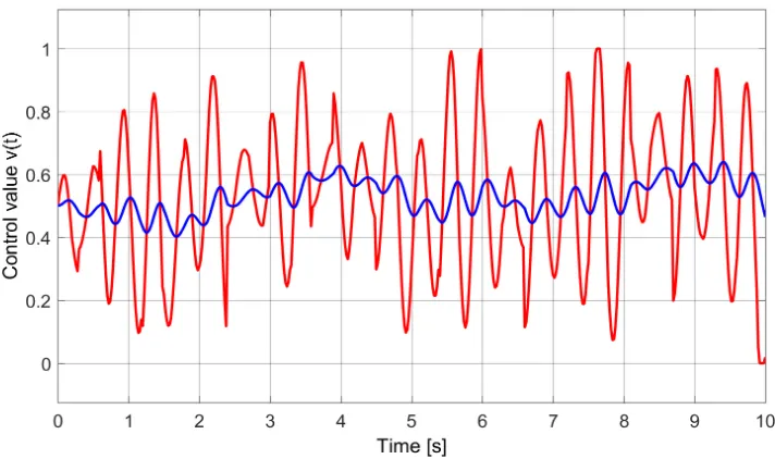
83

diagram of the final control element is shown in Figure 3.

84

Control valve Positioner

Pneumatic actuator

element Final control CV

e _Controller

System

SP

PVs

Instrument CVa

85

Figure 3. Block diagram of an electro-pneumatic final control element. Notions: CV – output of

86

external controller; CVI – output of internal controller; PC – internal controller;

87

E/P – electro-pneumatic transducer; PS – compressed air supply; pz - supply air pressure; ps - the

88

output pressure of the E/P transducer; X - displacement of the valve plug; XT – displacement

89

transducer of the actuator's rod; PXs - measured displacement of the actuator's rod [6].

90

When applied, one requires from the final control element a repetitive non-hysteresis static

91

characteristics, aperiodic step response and minimum control time. In principle, realisation of these

92

requirements becomes realistic only due to the use of a positioner.

93

It should be noted that the final control elements are exposed to adverse environmental

94

conditions such as thermal shocks, a wide range of operating temperatures, vibrations, humidity,

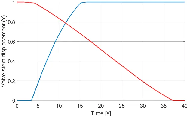
95

dusty pollutants, corrosive working environment and electromagnetic interference. Therefore, the

96

final control elements are classified as belonging to the group of elements of automation systems

97

subjected to the most frequent failures.It is estimated that among instrumentation, actuators and

98

technological components, the share of failures of final control elements exceeds 45%. The faulty

99

final control element can lead to a deterioration of the quality of the final product, and can even lead

100

to the process shut-down. All these factors influence the safety of the process and humans involved,

101

as well as worsen the economic indices of the process. For this reason, the assurance of the most

102

trouble-free operation of such devices becomes more important. In this context, the issues of fault

103

prediction and diagnostics, as well as ways of prevention actions and fault tolerant control become

104

particularly pertinent [7]. Most frequently, the electro-pneumatic transducer is subject to fail in case

105

of electro-pneumatic final control elements. This component fails due to poor quality of supply air,

106

friction wear of its mechanical components and material fatigue of its moving parts.

107

In this paper, a practical and economic approach to prolongation of final control element

108

lifetime is proposed. It is based on appropriate shaping and tuning of the positioner controller in

109

such a manner that it results in the limitation of the amplitude and of the number of cycles on its

110

output. This directly influences the wear and fatigue of moving elements of the electro-pneumatic

111

transducer. This type of approach, due to the conclusions drawn from the Wöhler’s fatigue curve [8],

112

has significant impact on mean-time-between-failures (MTBF), and therefore, reduces wear and

113

increases functional safety of the controlled process.

114

The essence of the proposed approach is to change the structure and parameters of the

115

positioner controller (PC) in order to minimize its effort, but not at the expense of worsening the

116

control quality factors of the controlled system in which such an element is used.

117

The results of research of the proposed approach were obtained in the Matlab-Simulink

118

simulation environment with the use of the final control element model [9] which is recognized

119

widely in the field of diagnostics and process safety. This to some extent enhances trustworthiness of

120

2. The controller effort

122

Before we discuss the problem of minimizing controller’s effort, let us define a few effort related

123

terms for the continuous and discrete time domain systems.

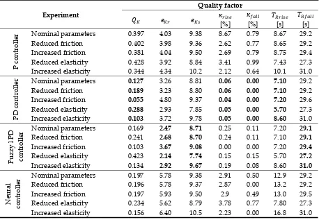
124

Definition 1. Define the normalized variability of the controller output 𝑣 𝑡 as:

125

𝑉 𝑡 = 1

∆𝑣 𝑑𝑣 𝑡

𝑑𝑡 , (1)

where: ∆𝑣 = |𝑣 − 𝑣 | – nominal range of controller output.

126

127

Definition 2. Define the controller's mean time effortover time interval ∆𝑡 as an average normalized

128

variability of the controller output.

129

𝑄 ∆𝑡 = 1

∆𝑡 𝑉 𝑡 𝑑𝑡 = 1 ∆𝑡 1 ∆𝑣 𝑑𝑣 𝑡

𝑑𝑡 𝑑𝑡, (2)

where: ∆𝑡 = 𝑡 − 𝑡 . By changing integration limits in (2), we can define cumulative time effort:

130

131

Definition 3. Define the controller's cumulative effortas an averaged over time normalized variability of the

132

controller output.

133

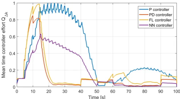
𝑄 𝑡 =1

𝑡 𝑉 𝑡 𝑑𝑡 = 1 𝑡 1 ∆𝑣 𝑑𝑣 𝑡

𝑑𝑡 𝑑𝑡. (3)

In the discrete time domain, the normalized variability can be expressed as:

134

𝑉 𝑘 = 1

∆𝑣 𝑣 − 𝑣 , (4)

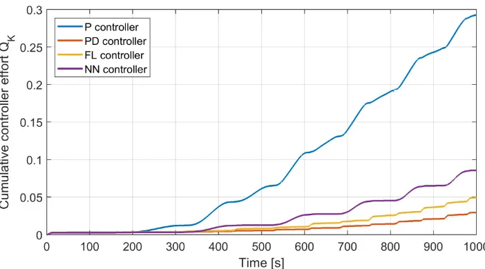
where: 𝑣 – k-th sample of the controller output 𝑣 𝑡 . By analogy to (2), the mean time effort in

135

discrete time domain can be expressed as the averaged sum of the variability of control signal over

136

the number of ∆𝑘 samples:

137

𝑄∆ =

𝑓

∆𝑘 − 1 𝑉 𝑘 =

1 ∆T

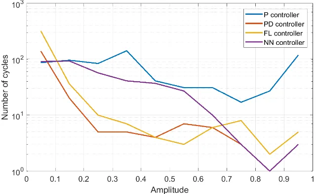
1

∆𝑣 𝑣 − 𝑣 . (5)

where: ∆𝑘 = 𝑘 − 𝑘 ; 𝑓 – sampling frequency of controller output 𝑣 𝑡 ; ∆𝑇 = _∆ – time

138

interval.

139

Remark: The introduction of sampling frequency 𝑓 in (5) avoids deflating/inflating effects of the

140

mean time effort for different sampling frequencies of the same control value.

141

Finally, by analogy to (3), the cumulative effort in the discrete time domain can be expressed as

142

the averaged sum of the variability of control signal over the 𝐾 samples:

143

𝑄 = 𝑓

𝐾 − 1 𝑉 𝑘 =

𝑓 𝐾 − 1

1

∆𝑣 𝑣 − 𝑣 =

1 𝑇

1

∆𝑣 𝑣 − 𝑣 , (6)

where: 𝑇 – time horizon. In practice, in automation systems, the control value is usually

144

normalized. In this case: ∆𝑣 = 1, and therefore respective formulas (1) - (6) appropriately simplify.

145

If we further assume that the movable elements of the electro-pneumatic transducer of

146

positioner approximately reproduce the trajectory of the control signal, then the reduction of the

147

controller's effort leads to a diminishing of the average amplitude and the totalized travel of its

148

moving elements. As a result, it is expected to reduce the intensity of wear of its mechanical

149

components and thus extends MTBF. Figure 4 presents an example of two control strategies for the

150

electro-pneumatic transducer: an aggressive marked with a red line and a conservative marked by

151

the dark blue line. The appropriate cumulative effort values for both strategies in the time horizon

152

eleven-fold reduction in the controller’s effort allows the increase of the permissible number of

154

work cycles due to the significant decrease of their amplitude.

155

156

Figure 4. An example of two control strategies with a strongly differentiated effort. Value of effort

157

for aggressive strategy QK=0.32 and for conservative strategy QK=0.029 [10].

158

3. Research environment

159

The implementation of experimental investigations in a real life scenario is usually costly and

160

time consuming. For this reason, the choice of the structure, parameters and tests of the proposed

161

control strategy was carried out in a simulation. For this purpose, was used a complex,

162

phenomenological model of an electro-pneumatic final control element. This model was prepared

163

and validated especially for assessment model based fault detection and isolation approaches [1].

164

The choice of this model was motivated by its availability [6] and the recognition in the

165

international community of process safety diagnostics. Simulation tests were performed by means of

166

the liquid level control system in which the final control element from [9] was applied. A simplified

167

block diagram of the simulated control system is shown in Figure 5.

168

169

Figure 5. Simplified simulation model of the liquid level control system. Notions: SP_L - level

170

setpoint; PV_L - measured level; CV_L - output of the main controller; SP - position setpoint of the

171

valve stem; PV - position of the valve stem; CV - output of the internal controller; X - position of the

172

valve stem; F - liquid flow rate; L - liquid level in the tank.

173

Applied final control element exhibits strong non-linearity, ambiguity and asymmetry of the

174

static characteristics (Figure 6). In addition, asymmetry and directionality of dynamic characteristics

175

177

Figure 6. Normalized static characteristics of pneumatic actuator of the electro-pneumatic final

178

control element.

179

180

Figure 7. Positive (blue line) and negative (red line) step response of the valve stem displacement of

181

pneumatic actuator.

182

It should be noted that the directionality of dynamic characteristics is a major challenge for the

183

internal positioner’s controller and has significant impact on its variability as well as on effort.

184

Directionality is clearly discernible in the parameter values of the effective transmittance of

185

pneumatic actuator.

186

𝐺 𝑠 = 1,6

12𝑠 + 1𝑒 ,

𝐺 𝑠 = 3

115𝑠 + 1𝑒

(7)

The dead time in the effective transmittance 𝐺 𝑠 results from a mechanical limitation of the

187

positioner’s rod movement and initial compression of the spring of the single-acting pneumatic

188

actuator. In turn, the dead time in the effective transmittance 𝐺 𝑠 follows from a mechanical

189

limitation of the positioner’s rod movement and time required to discharge the pressure in the

190

actuator chamber to the value at which a rod of the actuator begins the return stroke.

191

4. Control quality factors

193

Controller effort is just one of the many control quality factors used in order to evaluate the

194

features of automation systems [1-3]. Therefore, the minimizing of the effort of the controller

195

cannot be separated from the analysis of the impact on other control quality factors. There will be

196

seven control quality indicators analyzed in order to obtain a more complete view of the effects of

197

minimizing effort of the internal controller of positioner:

198

• cumulative effort of the controller 𝑄 according to formula (6) for T=100s;

199

• normalized, average absolute tracking error 𝑒 according to the formula (8). The value of this

200

factor is determined in test when applying a standardized trapezoidal setpoint SP shape with

201

the constant slope equal to 0.025s-1_.

202

𝑒 =𝑓

𝐾 |𝑆𝑃 𝑘 − 𝑋 𝑘 |, (8)

where: 𝑋 – positioner rod displacement;

203

• normalized, average absolute tracking error 𝑒 according to the formula (8). The value of this

204

factor is determined in a test in which a rectangular setpoint with the 5% amplitude and

205

period equal to 40s was applied.

206

• overshoots 𝜅 and 𝜅 obtained respectively for applying positive and negative 60%

207

stepwise function. Overshoot is defined as the ratio of the amplitude of the first transitional

208

control error 𝑒 to the setpoint change 𝑒 and expressed as a percentage.

209

𝜅 =𝑒

𝑒 (9)

• settling times: 𝑇 and 𝑇 for the 60% stepwise setpoint changes appropriately in positive

210

and negative direction Settling time is defined as the time which elapses from the moment of

211

the setpoint change until a positioner’s rod position X settles within ±0,05e tolerance band

212

around the steady state value.

213

5. Methodology

214

Without any doubt, the structure and parameters of internal positioner controller influences the

215

controller effort factors. This paper presents briefly the results of an experimental selection of the

216

structure and parameters of the internal controller of positioner for the control system shown in

217

Figure 4. The four different controller structures were studied namely: classic P and PD as well as

218

fuzzy PD and neural network one. The integral action was not considered in this case because of the

219

necessity of a guarantee system stability and hence assurance of sufficient gain and phase margins.

220

For all investigated control structures there are calculated values of all quality factors

221

presented in Section 4. It was assumed that tracking of the control value of the external controller is

222

the primary role of the final control element. For this reason, all controllers were tuned in order to

223

minimize value of mean absolute tracking error 𝑒 . Some reasonable practical limitations were

224

introduced. For example, the value of proportional gain was limited to 100.

225

The tests of internal positioner controller were carried out for:

226

• nominal values of friction and actuator’s spring elasticity;

227

• friction varying within the range [-50% , + 50%];

228

• actuator’s spring elasticity varying within the range [-50% , + 50%].

229

In order to minimize the simulation time, the tests were performed only for the extreme values

230

of the above mentioned influencing quantities.

231

6. Obtained results

235

The collected quality factors values obtained in the frames of performed simulation tests are

236

presented in Table 1. The best results are highlighted in bold.

237

Table 1. Experimentally obtained values of control quality factors.

238

Experiment

Quality factor

𝑄 𝑒 𝑒 𝜅

[%]

𝜅

[%]

𝑇

[s]

𝑇

[s]

P

con

tro

ller

Nominal parameters 0.397 4.03 9.38 8.67 0.79 8.67 29.2

Reduced friction 0.402 3.98 9.36 2.62 0.77 8.65 29.2

Increased friction 0.381 4.04 9.50 2.69 0.79 8.75 29.4

Reduced elasticity 0.428 3.92 8.84 3.41 0.99 7.43 27.3

Increased elasticity 0.344 4.34 10.2 2.12 0.64 10.1 31.0

PD

contro

lle

r _{Nominal parameters 0.127 3.26 8.81 0.06 0.00 7.10 29.2}

Reduced friction 0.189 3.23 8.80 0.06 0.00 7.10 29.2

Increased friction 0.055 4.80 9.37 0.04 0.00 7.20 29.6

Reduced elasticity 0.288 2.93 7.85 0.05 0.00 5.70 27.3

Increased elasticity 0.103 3.72 9.78 0.05 0.00 8.60 31.0

Fuzzy

l PD

controller

Nominal parameters 0.169 2.47 8.71 0.25 0.11 7.20 29.1

Reduced friction 0.241 2.68 8.70 0.24 0.11 7.10 29.1

Increased friction 0.103 3.67 9.08 0.00 0.00 7.20 29.4

Reduced elasticity 0.423 2.14 7.74 0.15 0.15 5.70 27.2

Increased elasticity 0.134 2.92 9.67 0.19 0.08 8.60 31.0

Neur

al

controller

Nominal parameters 0.197 5.78 9.38 2.91 0.50 12.9 29.2

Reduced friction 0.196 5.78 9.37 2.87 0.00 13.2 29.2

Increased friction 0.197 5.93 9.50 2.9 0.49 13.0 29.5

Reduced elasticity 0.234 5.62 8.79 3.78 0.77 7.80 27.3

Increased elasticity 0.156 6.40 10.5 2.23 0.00 16.8 31.0

239

6.1. Discussion of results

240

Table 1 provides interesting data for discussion. By comparing obtained results for different

241

types of controllers, it is possible to admit that classic proportional-and-derivative controller

242

provides the best control quality by minimal value of controller effort. This applies equally to classic

243

and fuzzy logic based controllers. In turn, neural network controller provides worse control quality

244

factors with comparable drop of the value of controller effort. The worst quality control factors were

245

obtained for proportional controller. The examples of the control outputs having lowest control

246

quality and the highest effort are shown in Figure 8. The outputs were recorded for the 0.0125Hz

247

trapezoidal setpoint excitation shape and the slope equal to 0.025s-1_{. In contrast, Figure 9 depicts the}

248

best results achieved for classic proportional-and-derivative and fuzzy logic controllers.

249

It is clear to see from Figure 8 that lowest control quality controllers generate a significant

250

number of high amplitude oscillations. Additionally, it negatively affects the lifetime of the

251

electro-pneumatic transducer itself and remaining parts of final control element. On the other hand,

252

the outputs of the PD and fuzzy logic controllers presented in Figure 9 are characterized by

253

relatively low number of quickly damped oscillations, which should be considered as highly

254

Figure 8. a) Output of P controller; b) Output of neural network controller.

256

Figure 9. a) Output of PD controller; b) Output of fuzzy logic PD controller.

257

The most important results inferred from the research carried out are shown in Figures 10-13.

258

The comparison of the mean time effort for all four controllers applied in the same control system

259

and working under the same conditions is shown in Figure 10. The mean time effort was calculated

260

here in moving time window with the width equal 10s. From this figure it comes that the principal

261

difference between controllers depends not on the short time effort but on the value of cumulative

262

effort over longer time. This is depicted clearly in Figure 11.

263

264

Figure 10. The comparison of the mean time effort of the four investigated controllers ∆𝑇 = 10𝑠 .

265

The cumulated effort of the four investigated controllers working under the same conditions is

266

268

Figure 11. The cumulative effort of the four investigated controllers in time horizon T=100s.

269

The cumulated effort was calculated for time horizon T varying from 0 to 100s. This plot allows

270

for the easiest and fastest evaluation of the choice of the proper structure of the internal controller

271

in terms of minimizing the effort and energy consumed from the auxiliary air supply source (Figure

272

3). This graph shows that in time window (up to 25s) the cumulative effort of

273

proportional-differentiating controllers is higher than for proportional controllers. However, from a

274

long - term perspective, the situation evidently changes.

275

It is also important to determine how the choice of the control strategy affects the durability

276

and fatigue of the electro-pneumatic transducer. The durability can be characterized indirectly by

277

the distribution of amplitude-cycles (A-S) curve. The appropriate graph for four tested controllers is

278

depicted in Figure 12. This graph was achieved by usage of chirp shaped setpoint. From this graph it

279

shows that controllers with a derivative action generate large number of cycles with relatively small

280

amplitude, and relatively low number of cycles having huge amplitudes. This observation allows

281

further consideration about the application of an additional filter for damping small amplitude

282

cycles. Quasi-constant A-S curve for proportional action controller gives an assumption to forecast

283

earlier fatigue of the driven electro-pneumatic transducer. It is also clear tosee from Figures 11

284

and 13 that in case of chirp setpoint, the cumulative effort of derivative action controllers is also

285

significantly smaller compared to others.

286

287

289

Figure 13. The cumulative effort of the four investigated controllers in 1000s time horizon and chirp

290

setpoint.

291

7. Summary

292

The three practical measures of the control quality that have been proposed in this paper are:

293

the variability, mean time and the cumulative effort of the controller. The simulation tests

294

demonstrate that with the proper selection of the structure and parameters of the internal controller

295

of the final control element, one can achieve two seemingly contradictory outcomes. On the one

296

hand, better quality control, while on the other, simultaneous reduction of the controller effort,

297

which in turn leads to a significant extension of the mean-time-between-failures of the

298

electro-pneumatic transducer. This is of great practical importance because the failures of

299

electro-pneumatic transducers are very prevalent in electro-pneumatic positioners. Additionally, it

300

also has economic benefits because it reduces the energy consumption by the actuators.

301

On the example of a fairly typical liquid level control system, it was shown that the

302

replacement of the algorithm of pneumatic actuator stem position controller from commonly used

303

classic P to PD or fuzzy PD allows more than a three-fold reduction of effort while simultaneously

304

obtaining much better values of quality control factors.

305

It is worth to mention, that frequently P controller is preferred in positioners. This comes from

306

considerations regarding cascade systems where the external controller performs integral action

307

and internal controller proportional action. As follows from the results of investigations presented

308

in this paper, it does not promise neither longer lifetime nor better control quality.

309

It would be advisable in the future to investigate the use of additional controller output

310

filtering to further reduce the actuator effort.

311

References

312

1. Manesis, S.; Nikolakopoulos, G. Introduction to Industrial Automation. Boca Raton, CRC Press, 2018.

313

2. Rodić, A.D. Automation & Control - Theory and Practice. Croatia, In-Tech, 2009.

314

3. Lipták, B.G. (Eds). Instrument Engineers' Handbook - Process Control and Optimization. Taylor & Francis, (2),

315

2006, pp. 2302.

316

4. Pneumatic control valve. Samson. Available online:

317

https://www.samson.de/en/products-applications/product-selector/valves/3321-pneumatic-din/

318

5. Globe Control Valve. Samson: http://www.samsoncontrols.com/product/3241-globe-control-valve.

319

6. DAMADICS RTN Information Website. Available online: diag.mchtr.pw.edu.pl/damadics.

320

7. Blanke, M.; Kinnaert, M.; Lunze, J.; Staroswiecki, M. Diagnosis and Fault-Tolerant Control, Springer, 2016.

321

9. Bartyś, M.; Patton, R.; Syfert, M.; de las Heras, S.; Quevedo, J. Introduction to the DAMADICS actuator

323

FDI benchmark study. Control Engineering Practice 2006, 14(6) pp. 577-596.

324

10. Hryniewicki, B. Development of the control strategy for a highly non-linear and non-stationary final control

325

element. Master thesis: AR_2_st_258971. Warsaw University of Technology, Faculty of Mechatronics, 2018,

326

pp. 1-100, (in polish).

327

328

Author Contributions:

329

Conceptualization, Michał Bartyś; Data curation, Bartłomiej Hryniewicki; Formal analysis, Michał Bartyś;

330

Investigation, Bartłomiej Hryniewicki; Methodology, Michał Bartyś; Project administration, Michał Bartyś;

331

Resources, Bartłomiej Hryniewicki; Software, Bartłomiej Hryniewicki; Supervision, Michał Bartyś;

332

Visualization, Michał Bartyś and Bartłomiej Hryniewicki; Writing – original draft, Michał Bartyś; Writing –

333

review & editing, Michał Bartyś.

334

Funding

335

Conflicts of Interest

336

the study; in the collection, analyses, or interpretation of data; in the writing of the manuscript, or in the

337