An Overview of Machine Learning, Deep Learning and Neural Networks

(1)

CSEIT1833384 | Received : 05 April 2018 | Accepted : 20 April 2018 | March-April-2018 [ (3 ) 3 : 1590-1595]

An Overview of Machine Learning, Deep Learning and Neural

Networks

Pranav Murali

SRM University, Electronics and Communication, Chennai, India

ABSTRACT

Every year millions of data are being generated by people around the world and they have to be processed quickly and efficiently. Mistakes could be made by humans but a computer or a system with a function to perform ,will never. So , it is essential for us to help the computer around us to do tasks that we humans take much more time to implement. This paper covers the picture of the much spoken about machine learning, deep learning and neural networks. At the end of this paper , we will have an understanding of these technologies and a good grasp of the process behind it.

Keywords: Algorithms, regression, computation, networks, neurons, training, data

I. INTRODUCTION

Machine Learning

Machine Learning is a process where a system learns from experience, data and follows instructions to make decisions intuitively and effectively without the need of an actual human. The computer has certain types of algorithms known as Machine Learning Algorithms which are used to solve the problems. There are a few popular algorithms such as

 Logistic Regression

 Nearest Neighbour

 Support Vector Machines

 Decision Trees

We shall talk about these algorithms one by one. But before that, we need to know the essential parameters required for the system to use these machine learning algorithms. The computer can’t just start using these algorithms with a set of input data. It’s not enough if data alone is given to the system but other vital parameters need to be computed and assigned before implementing the algorithm. There are steps involved in a machine learning process such as

 Gathering data : Getting data from multiple sources

 Data Preparation/Manipulation : Merging and converting raw data into user-defined

 Model decision : Decide model based on data such as text/music/sequence/imagery

 Training : Test the model with the data available

 Evaluation : Evaluate the results with respect to the error rate

 Tuning of parameters : Tune the parameters to get the least error rate and best results

 Prediction : Predict the favourable outcome

Logistic Regression

(2)

Figure 1. Regression

Nearest Neighbour

Consider a situation where a variable is given in a 2-Dimensional space and we are supposed to find where it belongs and to which class it belongs. This is an important concept because only when the machine understands where a variable or a parameter belongs, it can categorize the information accurately and helps in better prediction.

Figure 2. Nearest Neighbour plot

Nearest Neighbour is also known as k-NN algorithm where k identifies the nearest neighbours. Consider the above picture, we can see that c is the variable and ‘a’ and ‘o’ are the two different classes. We also see that k=3 and we use this algorithm to find the class of ‘c’. This situation is relatively simple and we see that ‘o’ is the class since there are 2 Os closer to c and only 1 A but in general, we have a formula to determine the class of c which is

Figure 3. Equation of weights of system

Where W function is the system of giving weights to all the points around the variable and determines the relative closeness of each neighbour with respect to the query point. Weights are being used because we assume objects close to each other are similar in nature and also the closest point would have more influence towards the outcome of the system.

Support Vector Machines

In this algorithm, we classify a given set of data as belonging to one or more set of categories. Suppose a training data is given, we use this algorithm to build a model and assign examples to the data. Mapping of the new assigned data with examples is done , which further leads to a representation of all the points in space where the categories are separated by a margin as big as possible. This representation of data in the form of categories ( with assigned examples ) and separation with a margin as big as possible leads to easy prediction of results because we can easily segregate data belonging to specific categories.

Figure 4. Support Vector Machines plot

(3)

Bio-medical fields use SVMs for protein classification. Based on the side of the gap the data falls, categories are predicted.

Decision Trees

A decision tree is nothing but a collection of all the possible results ( outcomes ) when compared to one another in various situations and weighing them correspondingly. It involves factors such as costs , probabilities to plot a decision tree. Decision trees can be drawn using flowcharts or nodes according to the user requirements and understanding capability. Decision tree helps us in classification of a variable which lead to objective results. It has certain advantages like being easy to understand , imparting several other factors in a tree branch when required and mapping of data without much preparation in the initial stages , thus saving a lot of time.

Bagging , Random forest classifiers are examples of types of decision trees that help in classification of data , sampling them and help in reaching decisions. Big picture about machine learning is that these algorithms are used as classifiers to give labels to each set of data and further use mathematics ( probability and statistics ) to assign equations and calculate error rate , weight towards output etc..and fit the best model. Once the algorithm is decided, the machine learning steps as mentioned earlier take place one at a time and we get the results. of neurons. Each neuron in a cell consists of 3 main components: Soma ( body of a neuron ) , Dendrite ( arms of a neuron ) and the Axon ( tail of a neuron ).

Any electrical activity the body possesses is picked up by the dendrite and sent to the Soma. The Soma then further sends this signal to the axon for activity and response. Interconnection between neurons is done by Synapse ( axon of one to dendrite of another ). So, in this way connection between neurons can be strong , medium and weak. Input neurons give output neurons according to the weight of the input neurons given initially.

So what we do from here on is initially gather data.

 Gathering of data

Once data is gathered we need to represent the information in the form of input and output neurons. We don’t have to worry about the weights of the input neurons , the system will take care of it. We randomly assign weights to the neurons but we have to give the possible output neuron parameters.

Then we calculate the error, if the activity ( axon to dendrite signal ) between neurons is 1 , it means the weights assigned are good. If the activity is bad , then the weights need to be updated.

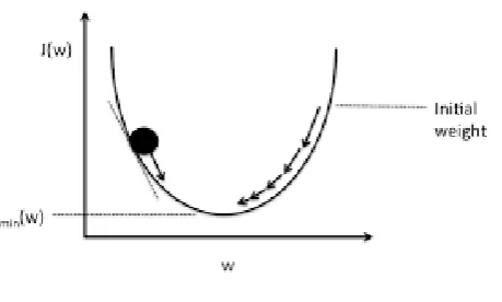
 Gradient Descent

For weights to be updated, we follow the gradient descent method in deep learning. It’s a simple plot of error vs weight and we adjust the weight up and down , check how the error corresponds to each movement.

(4)

As you can see from the figure, the graph shows the plot of gradient descent. The point at which we reach Jmin(W) is the ideal point.

 Back-Propagation

The next step is back-propagation. This is where the weights are adjusted especially the ones with least weight because there is bias towards the neurons with high weights and this causes irregularities.

Figure 6. Back-Propagation

So the above figure is a typical example of how layers of neurons are adjusted so as to get proper biasing of output neurons and appropriate results.

 Deep Network

Now, if a network has more than 3 layers then it is called a deep network. It’s complex in nature and is used for example in image recognition. Take for instance the first layer of input neurons, the pixels are given. The second layer is a combination of all the first layer neurons, we may get eyes. The third layer may get us lips. The fourth maybe nose and so the layers keep getting deep and deep and the neuron layers are complex in nature.

Figure 7. Deep Learning Process

This photo shows how deep learning with layers of networks works for a facial recognition system. From random pixels to final image processing, the neuron network consists of many layers and we use neural network transformations to carry out the processes. So , the next section about neural networks will cover those processes.

III. NEURAL NETWORKS

Neural networks are the message carrying signals of the machine/deep learning process. There are various kinds of neural networks used in our systems. However, we would be talking about the widely used ones which can be incorporated into any model.

 Convolution Neural Networks(CNN)

These are multi layer neural networks used mainly for facial recognition. Let’s assume we have a 2-Dimensional image given as input and the objective is to find out if each pixel present in the image has a ‘X’ or an ‘O’. Now , the basic working of a neural network in the system would be to analyse the value of each pixel. Let’s say the value of pixel X is 1 and that of pixel O is -1. So, the computer individually recognizes the pixels. But, the overall pattern of the image might not make it easier to identify the features of this image.

Figure 8. Computer assumption of pixels

(5)

of the image with each other as you can see in the below diagram

Figure 9. Working of pixels in CNN

This matching is done by using a part of the feature and comparing it to the mapped image done previously.

Figure 10. Filtering in CNN

As you can see, the feature on the top left is compared with an image of X in a 2-Dimensional image mapped previously by the system as default. The math behind the filtering is simple:

Line up the feature and image patch, multiply each pixel by the corresponding image pixel, Add them up and divide by the total number of pixels in the feature. This is carried out across all layers and pixels of the image and when we do that, it becomes convolution. In the end, repeated process of filtering is what we call convolution.

 Feed Forward Neural Networks

These are the simplest form of networks. Used for speech recognition systems. Input layer comes first, followed by intrinsic hidden layers and then the output layers at the end as we go up.

For speech recognition, we need different things said by the same speaker to be dissimilar while same things said by different speakers to be classified similar. Transformations take place between each layer and non-linearity exists between layers of neurons.

Figure 11. Feed Forward Neural Network

 Recurrent Networks

These are networks with directed cycles in their connection. By following the arrows, one can get to the starting point of the data set if needed. They are complicated compared to feed forward network and so are difficult to train. Due to their connectivity, biologically they are more realistic. They have the ability to remember information for a long time in their hidden states.

(6)

IV. CONCLUSION

Thus this paper concludes with the discussion of these popular neural networks. We now have an overall picture of machine learning, deep learning and how it works with the help of neural networks implemented in computation systems to generate results. We saw about the algorithms of machine learning and how such algorithms could be introduced into the process. We then dived into the more complicated deep learning and how a design just like neurons in our nervous system are implemented in systems to form networks and give results.

V. REFERENCES

[1].Jensen, F. V. (1996). An introduction to Bayesian networks

[2].Han, J., & Kamber, M. (2001). Data mining: Concepts and techniques

[3].R Raina A Madhavan AY Ng. Large-scale deep unsupervised learning using graphics processorsJ].

[4].Logistic Regression

http://www.learnbymarketing.com/methods/logi stic-regression-explained/

[5].Nearest Neighbours

http://www.statsoft.com/Textbook/k-Nearest-Neighbors

[6].Data science comparison with big data , https://www.simplilearn.com/data-science-vs-bigdata-vs-data-analytics-article

[7]. E-learning industry,