1338
Sequential Graph Dependency Parser
Sean Welleck New York University
Kyunghyun Cho New York University CIFAR Azrieli Global Scholar
Facebook AI Research
Abstract
We propose a method for non-projective dependency parsing by incrementally pre-dicting a set of edges. Since the edges do not have a pre-specified order, we pro-pose a set-based learning method. Our method blends graph, transition, and easy-first parsing, including a prior state of the parser as a special case. The pro-posed transition-based method success-fully parses near the state of the art on both projective and non-projective languages, without assuming a certain parsing order.
1 Introduction
Dependency parsing methods can be categorized as graph-based and transition-based. Typical graph-based methods support non-projective pars-ing, but introduce independence assumptions and rely on external decoding algorithms. Conversely, transition-based methods model joint dependen-cies, but without modification are typically limited to projective parses.
There are two recent exceptions of interest here. (Ma et al., 2018) developed the Stack-Pointer parser, a transition-based, non-projective parser that maintains a stack populated in a top-down, depth-first manner, and uses a pointer network to determine the dependent of the stack’s top node, resulting in a transition sequence of length2n−
1. Recently, (Fern´andez-Gonz´alez and G´omez-Rodrguez,2019) developed a variant of the Stack-Pointer parser which parses innsteps by travers-ing the sentence left-to-right, selecttravers-ing theheadof the current node in the traversal, while incremen-tally checking for, and prohibiting, cycles.
We take inspiration from both graph-based and
transition-based approaches by viewing parsing as sequential graph generation. In this view, a graph is incrementally built by adding edges to an edge set. No distinction between projective and non-projective trees is necessary. Since edges do not have a pre-specified order, we propose a set-based learning method. Like ( Fern´andez-Gonz´alez and G´omez-Rodrguez,2019), our parser runs in n steps. However, our learning method and transitions do not impose a left-to-right pars-ing order, allowpars-ing easy-first (Tsuruoka and Tsu-jii,2005;Goldberg and Elhadad,2010) behavior. Experimentally, we find that the proposed method can yield a sequential parser with preferred, input-dependent generation orders and performance gains over strong one-step methods.1
2 Graph Dependency Parser
Given a sentencex = x1, . . . , xN, a dependency
parser constructs a graphG = (V, E) with V = (x0, x1, . . . , xN) and E = {(i, j)1, . . .(i, j)N},
wherex0 is a special root node, andE⊂ E forms a dependency tree.2
We describe a family of sequential graph-based dependency parsers. A parser in this family gen-erates asequenceof graphs whereV is fixed and
E=ST t=1Et:
Henc=fenc(x0, . . . xN) (1)
Hthead, Htdep=fV(Henc, E<t, ht−1) (2)
St=fE(Hthead, H dep
t , St−1) (3)
Et=fdec(St, E<t). (4)
Steps (2-4) run forT ≤ N time-steps. At each time-step, firstfV generates head and dependent
1
Code will be made available athttps://github. com/wellecks/nonmonotonic_parsing.
representations for each vertex, Ht· ∈ RV×dH,
based on vertex representations Henc ∈ RV×d, previously predicted edges E<t, and a recurrent
stateht−1 ∈ Rd. ThenfE computes a score for
every possible edge,St ∈ RV×V, and the scores are used byfdecto predict a set of edgesEt.
This general sequential family includes the bi-affine parser of (Dozat and Manning, 2017) as a one-step special case, as well as a recurrent vari-ant which we discuss below.
2.1 Biaffine One-Step
The Biaffine parser of (Dozat and Manning,2017) is a one-step variant, implementing steps (1-4) us-ing a bidirectional LSTM, head and dependent neural networks, a biaffine scorer, and a maximum spanning tree decoder, respectively:
Henc=BiLSTM(x1, . . . , xN)
Hhead, Hdep =MLPh(Henc),MLPd(Henc)
S =BiAffine(Hhead, Hdep)
E =MST(S),
where each row of scores S(i) is interpreted as a distribution overi’s potential head nodes:
p((j →i)|x)∝softmaxj(S(i)),
and MST(·) is an off-the-shelf maximum-spanning-tree algorithm. This model assumes conditional independence of the edges.
2.2 Recurrent Weight
We propose a variant which iteratively adjusts a distribution over edges at each step, based on the predictions so far. A recurrent function generates a weight matrix W which is used to form vertex embeddings and in turn adjust edge scores.
Specifically, we first obtain an initial score matrix
S0using the biaffine one-step parser (2.1), and ini-tialize a recurrent hidden state h0 using a linear transformation of fenc’s final hidden state. Then fV is defined as:
W, ht=LSTM(femb(Et−1), ht−1)
Hthead=embh(0, . . . , N)W
Htdep=embd(0, . . . , N)W,
andfE(Hthead, H dep
t , St−1)is defined as:
S∆t =BiAffine(Hthead, Htdep)
St=St−1+St∆,
wheretranges from 1 toN,W ∈ Rdemb×dH, and
each emb(·) : N→ Rdemb is a learned embedding layer, yielding emb(·)(0, . . . , N)inRV×demb. We use a bidirectional LSTM asfenc.
The scores at each step yield a distribution over all
V ×V edges, which we denote byπ:
π((i→j)|E<t, x)∝softmax(flatten(St)). (5)
Unlike the one-step model, this recurrent model can predict edges based on past predictions.
Inference We must ensure the incrementally de-coded edges E = ST
t=1Et form a valid
depen-dency tree. To do so, we choosefdec to be a de-coder which greedily selects valid edges,
Et=fvalid(St, E<t),
which we refer to as the valid decoder, detailed in AppendixA. We only predict one edge per step
(|Et|= 1), leaving the setting of multiple
predic-tions per step as future work.
Embedding Edges We embed a predicted edge
Et={(i, j)ˆ }as:
femb(Et) =eedge;ehead;edependent eedge=WeH(enci) −WeH(encj)
ehead=embh(i) edependent=embd(j),
whereH(enc·) ∈ Rd are row vectors,W
e ∈ Rde×d is a learned weight matrix, emb(·)are learned em-bedding layers, and;is concatenation.
Future Work The proposed method does not specifically require a BiLSTM encoder, LSTM, or the BiAffine function. For instance, fV could use a Transformer (Vaswani et al., 2017) to out-put states that are linearly transformed intoHhead
and Hdep. Additionally, partial graphs (V, E <t)
edges’ objective, similar to recent work in ma-chine translation with conditional masked lan-guage models (Ghazvininejad et al.,2019). Each call tofV would involve a separate forward pass
which calls a Transformer fenc. The partial tree is encoded via non-masked inputs tofenc. fE
cor-responds to havingV outputs, each a distribution overV edges. The multi-step decoder (Appendix
A) might be used at test time.
3 Learning
In this paper, we restrict to the case of predict-ing a spredict-ingle edge(i, j)ˆ per step, so that the recur-rent weight model generates a sequence of edges with the goal of matching a target edge set, i.e.
SN
t=1(i, j)ˆ t = E. Since the target edgesE are a
set, the model’s generation order is not determined a priori. As a result, we propose to use a learning method that does not require a pre-specified gen-eration order and allows the model to learn input-dependent orderings.
Our proposed method is based on the multiset loss (Welleck et al.,2018) and its recent extensions for non-monotonic generation (Welleck et al.,2019). The method is motivated from the perspective of learning-to-search (Daum´e III et al.,2009;Chang et al.,2015), which involves learning apolicyπθ
that mimics anoracle policyπ∗. The policy maps statesto distributions overactions.
For the proposed graph parser, an action is an edge
(i, j) ∈ E, and a state st is an input sentence x
along with the edges predicted so far, Eˆ<t. The
policy is a conditional distribution overE,
πθ((i, j)|Eˆ<t, x),
such as the distribution in equation (5).
Learning consists of minimizing a cost, computed by first sampling states from a roll-inpolicyπin, then using a roll-out policyπout to estimate cost-to-go for all actions at the sampled states. For-mally, we minimize the following objective with respect toθ:
Ex∼DEs1,...,s|x|∼πinC(πθ, π
out, s
t). (6)
This objective involves sampling a sentence x
from a dataset, sampling a sequence of edges from the roll-in policy, then computing a cost C at each of the resulting states. We now describe
our choices of C, πout, π∗, andπin, and evaluate
them later in the experiments (4).
3.1 Cost Function and Roll-Out
Following (Welleck et al., 2018, 2019) we use a KL-divergence cost:
C(πθ, πout, s) =DKL(πout(·|s)||πθ(·|s)). (7)
We use the oracleπ∗ as the roll-outπout.
3.2 Oracle
Based on the free labels set in (Welleck et al.,
2018), we first define a free edge set containing the un-predicted target edges at timet:
Efreet =E\
t−1
[
t0=1
ˆ
(i, j)t0, (8)
where E0
free = E. We then construct a family
of oracle policies that place non-zero probability mass only on free edges:
π∗((i, j)|Efreet ) = (
pij (i, j)∈Efreet
0 otherwise. (9)
We now describe several oracles by varying how
pij is defined.
Uniform This oracle treats each permutation of the target edge set as equally likely by assigning a uniform probability to each free edge:
πunif∗ ((i, j)|Efreet ) =
( 1
|Et
free|
(i, j)∈Efreet
0 otherwise.
Coaching Motivated by (He et al., 2012;
Welleck et al.,2019), we define a coaching oracle which weights free edges byπθ:
πcoaching∗ ((i, j)|Efreet )∝πunif∗ (·|Efreet )πθ(·|E<t, X).
This oracle prefers certain edge permutations over others, reinforcingπθ’s preferences. The coaching
and uniform oracles can be mixed to ensure each free edge receives probability mass:
βπunif∗ + (1−β)πcoaching∗ , (10)
Annealed Coaching This oracle begins with the uniform oracle, then anneals towards the coach-ing oracle as traincoach-ing progresses by annealcoach-ing the
β term in (10). This may prevent the coaching oracle from reinforcing sub-optimal permutations early in training.
Linearized This oracle uses a deterministic function to linearize an edge setEinto a sequence
Eseq. The oracle selects thet’th element ofEseqat
timetwith probability 1. We linearize an edge set in increasing edge-index order: (i1, j1) precedes
(i2, j2)if(i1, j1) <(i2, j2). This oracle serves as a baseline that is analogous to the fixed generation orders used in conventional parsers.
3.3 Roll-In
The roll-in policy determines the state distribution thatπθ is trained on, which can address the
mis-match between training and testing state distribu-tions (Ross et al.,2011;Chang et al.,2015) or nar-row the set of training trajectories. We evaluate several alternatives:
1. uniform(i, j)∼πunif∗
2. coaching(i, j)∼πθπunif∗
3. valid-policy(i, j)∼valid(πθ)
where valid(πθ)is the set of edges that keeps the
predicted tree as a valid dependency tree. The coaching and valid-policy roll-ins choose edge permutations that are preferred by the policy, with valid-policy resembling test-time behavior.
4 Experiments
In Experiments 4.1 and 4.2 we evaluate on En-glish, German, Chinese, and Ancient Greek since they vary with respect to projectivity, size, and per-formance in (Qi et al.,2018). Based on these de-velopment set results, we then test our strongest model on a large suite of languages (4.3).
Experimental Setup Experiments are done us-ing datasets from the CoNLL 2018 Shared Task (Zeman et al.,2018). We build our implementa-tion from the open-source version of (Qi et al.,
2018)3, and use their experimental setup (e.g.
3https://github.com/stanfordnlp/
stanfordnlp.
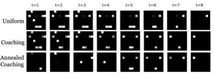
Figure 1: Per-step edge distributions from recur-rent weight models trained with the given oracle.
pre-processing, data-loading, pre-trained vectors, evaluation) which follows the shared task setup. Our model uses the same encoder from (Qi et al.,
2018). For the (Qi et al.,2018) baseline, we use their pretrained models4and evaluation script. For the (Dozat and Manning,2017) baseline, we use the (Qi et al., 2018) implementation with auxil-iary outputs and losses disabled, and train with the default hyper-parameters and training script. For our models only, we changed the learning rate schedule (and model-specific hyper-parameters), after observing diverging loss in preliminary ex-periments with the default learning rate. Our mod-els did not require the additional AMSGrad tech-nique used in (Qi et al.,2018). We evaluate vali-dation UAS every 2k steps (vs. 100 for the base-line). Models are trained for up to 100k steps, and the model with the highest validation unlabeled at-tachment score (UAS) is saved.
4.1 Multi-Step Learning
In this experiment we evaluate the sequential as-pect of the proposed recurrent model by compar-ing it with one-step baselines. We compare against a baseline (‘One-Step’) that simply uses the first step’s score matrix S0 from the recurrent weight model and minimizes (6) for one time-step using a uniform oracle. At test time the valid decoder usesS0for all timesteps. We also compare against the biaffine one-step model of (Dozat and Man-ning,2017) which uses Chu-Liu-Edmonds maxi-mum spanning tree decoding instead of valid de-coding. Since we only evaluate UAS, we disable its edge label output and loss. Finally, we com-pare against (Qi et al., 2018) which is based on (Dozat and Manning, 2017) plus auxiliary losses for length and linearization prediction.
Results are shown in Table1, including results for
4https://stanfordnlp.github.io/
En De Grc Zh
D & M (2017) 91.14 90.38 78.99 86.50
Qi et al.(2018) 92.11 89.46 81.35 86.73 One-Step 91.74 91.07 79.60 86.61 Recurrent (U) 91.92 91.02 79.15 86.69 Recurrent (C) 91.99 91.19 79.93 86.77
Table 1: Development set UAS for single vs. multi-step methods. (U) is uniform oracle and roll-in, (C) is coaching with greedy valid roll-in (β = 0.5). D & M (2017)is an abbreviation for (Dozat and Manning,2017).
a recurrent model trained with coaching (‘Recur-rent (C)’) using a mixture (eq. 10) withβ = 0.5. The one-step baseline is strong, even outperform-ing the uniform recurrent variant on some lan-guages. The recurrent weight model with coach-ing, however, outperforms the one-step and (Dozat and Manning, 2017) baselines on all four lan-guages. Adding in auxiliary losses to the (Dozat and Manning,2017) model yields improved UAS as seen in the (Qi et al.,2018) performance, sug-gesting that our proposed recurrent model might be improved further with auxiliary losses.
Temporal Distribution Adjustment Figure 1
shows per-step edge distributions on an eight-edge example. The recurrent weight variants learned to adjust their distributions over time based on past predictions. The model trained with the uniform oracle has a decreasing number of high probabil-ity edges per step since it aims to place equal mass on each free edge(i, j)∈Eˆfreet . The model trained with coaching learned to prefer certain free edges over others, but with β = 0.5 the uniform term in the loss still encourages placing mass on multi-ple edges per step. By annealingβ, however, the coaching model exhibits vastly different behavior than the uniform-trained policy. The low entropy distributions at early steps followed by higher en-tropy distributions later on (e.g. t ∈ {5,6}) may indicate easy-first behavior.
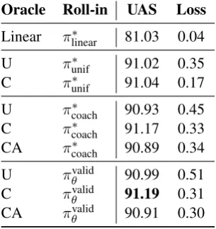
4.2 Oracle and Roll-In Choice
In this experiment, we study the effects of vary-ing the oracle and roll-in distributions. Table (2) shows results on German, analyzed below. Mod-els trained with coaching (C) use a mixture with
β = 0.5, after observing lower UAS in
prelim-Oracle Roll-in UAS Loss
Linear π∗linear 81.03 0.04
U π∗unif 91.02 0.35 C π∗unif 91.04 0.17
U π∗coach 90.93 0.45
C π∗coach 91.17 0.33
CA π∗coach 90.89 0.34
U πvalidθ 90.99 0.51
C πvalid
θ 91.19 0.31
CA πvalidθ 90.91 0.30
Table 2: Varying oracle and roll-in policies on German. (U), (C), (A) refer to uniform, coaching, and annealing, respectively. Theπ∗coachandπvalid
θ
roll-ins are mixtures with a uniform oracle, with
β = 0.5for coaching (C), andβlinearly annealed by 0.02 every 2000 steps for annealing (CA).
inary experiments with lower β. The πcoach∗ and
πθvalid roll-ins use a mixture with β = 0.5 and greedy decoding, which generally outperformed stochastic sampling.
Set-Based Learning The model trained with the linearized oracle (UAS 81.03), which teaches the model to adhere to a pre-specified generation order, significantly under-performs the set-based models (UAS ≥ 90.89), which do not have a pre-specified generation order and can in principle learn strategies such as easy-first.
Coaching Models trained with coaching (C, UAS ≥ 91.04) had higher UAS and lower loss than models trained with the uniform oracle (U, UAS≤ 91.02), for all roll-in methods. This sug-gests that for the proposed model, weighting free edges in the loss based on the model’s distribution is more effective than a uniform weighting.
Annealing the β parameter generally did not fur-ther improve UAS (CA vs. C), possibly due to the annealing schedule or overfitting; despite lower losses with annealing, eventually validation UAS decreasedas training progressed.
Roll-In With the coaching oracle (C), the choice of roll-in impacted UAS, with coaching roll-in (π∗coach, 91.17) and valid roll-in (πθvalid,91.19)
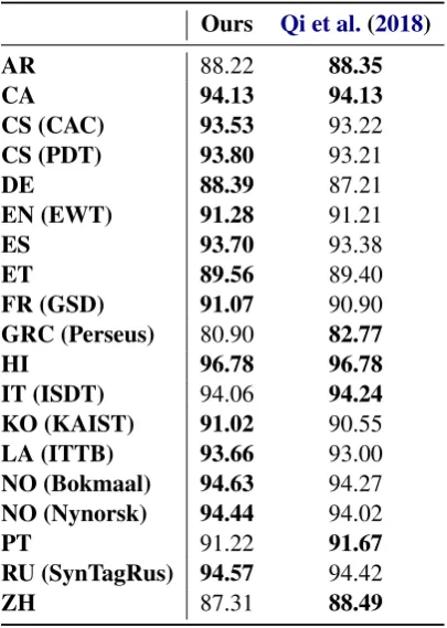
Ours Qi et al.(2018)
AR 88.22 88.35
CA 94.13 94.13
CS (CAC) 93.53 93.22
CS (PDT) 93.80 93.21
DE 88.39 87.21
EN (EWT) 91.28 91.21
ES 93.70 93.38
ET 89.56 89.40
FR (GSD) 91.07 90.90
GRC (Perseus) 80.90 82.77
HI 96.78 96.78
IT (ISDT) 94.06 94.24
KO (KAIST) 91.02 90.55
LA (ITTB) 93.66 93.00
NO (Bokmaal) 94.63 94.27
NO (Nynorsk) 94.44 94.02
PT 91.22 91.67
RU (SynTagRus) 94.57 94.42
ZH 87.31 88.49
Table 3: Test set results (UAS) on datasets from the CoNLL 2018 shared task with greater than 200k examples, plus the Ancient Greek (GRC) and Chinese (ZH) datasets. Bold denotes the high-est UAS on each dataset.
to those preferred by the policy may be more ef-fective than sampling uniformly from the set of all correct trajectories. Based on these results, we use the coaching oracle and valid roll-in for training our final model in the next experiment.
4.3 CoNLL 2018 Comparison
In this experiment, we evaluate our best model on a diverse set of multi-lingual datasets. We use the CoNLL 2018 shared task datasets that have at least 200k examples, along with the four datasets used in the previous experiments. We train a recurrent weight model for each dataset using the coaching oracle and valid roll-in. We compare against (Qi et al., 2018) which placed highly in the CoNLL 2018 competition, reporting test UAS evaluated using their pre-trained models.
Table 3 shows the results on the 19 datasets from 17 different languages. The proposed model trained with coaching achieves a higher UAS than theQi et al.(2018) model on 12 of the 19 datasets, plus two ties.
5 Related Work
Transition-based dependency parsing has a rich history, with methods generally varying by the choice of transition system and feature represen-tation. Traditional stack-based arc-standard and arc-eager (Yamada and Matsumoto, 2003;Nivre,
2003) transition systems only parse projectively, requiring additional operations for pseudo-non-projectivity (G´omez-Rodr´ıguez et al., 2014) or projectivity (Nivre, 2009), while list-based non-projective systems have been developed (Nivre,
2008). Recent variations assume a generation or-der such as top-down (Ma et al.,2018) or left-to-right (Fern´andez-Gonz´alez and G´omez-Rodrguez,
2019). Other recent models focus on unsuper-vised settings (Kim et al.,2019). Our focus here is a non-projective transition system and learning method which does not assume a particular gener-ation order.
A separate thread of research in sequential mod-eling has demonstrated that generation order can affect performance (Vinyals et al.,2015), both in tasks with set-structured outputs such as objects (Welleck et al., 2017, 2018) or graphs (Li et al.,
2018), and in sequential tasks such as language modeling (Ford et al., 2018). Developing mod-els with relaxed or learned generation orders has picked up recent interest (Welleck et al., 2018,
2019;Gu et al.,2019;Stern et al.,2019). We in-vestigate this for dependency parsing, framing the problem as sequential set generation without a pre-specified order.
Finally, our work is inspired by techniques for improving upon maximum likelihood training through error exploration and dynamic oracles (Goldberg and Nivre, 2012, 2013), and related techniques in imitation learning for structured pre-diction (Daum´e III et al.,2009;Ross et al.,2011;
He et al., 2012; Goodman et al., 2016). In par-ticular, our formulation is closely related to the framework of (Chang et al.,2015), where our ora-cle can be seen as an optimal roll-out policy which computes action costs without explicit roll-outs.
6 Conclusion
Yoshimasa Tsuruoka and Jun’ichi Tsujii. 2005. Bidi-rectional inference with the easiest-first strategy for
tagging sequence data. In Proceedings of the
con-ference on human language technology and empirical methods in natural language processing, pages 467– 474. Association for Computational Linguistics.
Ashish Vaswani, Noam Shazeer, Niki Parmar, Jakob Uszkoreit, Llion Jones, Aidan N Gomez, Ł ukasz
Kaiser, and Illia Polosukhin. 2017. Attention is all you
need. InAdvances in Neural Information Processing Systems 30, pages 5998–6008. Curran Associates, Inc.
Oriol Vinyals, Samy Bengio, and Manjunath Kudlur.
2015.Order Matters: Sequence to sequence for sets.
Sean Welleck, Kiant Brantley, Hal Daum III, and
Kyunghyun Cho. 2019. Non-monotonic sequential text
generation.
Sean Welleck, Kyunghyun Cho, and Zheng Zhang. 2017. Saliency-based sequential image attention with
multiset prediction. InAdvances in neural information
processing systems.
Sean Welleck, Zixin Yao, Yu Gai, Jialin Mao, Zheng Zhang, and Kyunghyun Cho. 2018. Loss functions for
multiset prediction. InAdvances in Neural Information
Processing Systems, pages 5788–5797.
H. Yamada and Y. Matsumoto. 2003. Statistical De-pendency Analysis with Support Vector machines. In
The 8th International Workshop of Parsing Technolo-gies (IWPT2003).
Daniel Zeman, Jan Hajiˇc, Martin Popel, Martin Pot-thast, Milan Straka, Filip Ginter, Joakim Nivre, and
Slav Petrov. 2018.CoNLL 2018 shared task:
Multilin-gual parsing from raw text to universal dependencies. InProceedings of the CoNLL 2018 Shared Task: Mul-tilingual Parsing from Raw Text to Universal Depen-dencies, pages 1–21, Brussels, Belgium. Association for Computational Linguistics.
A Sequential Valid Decoder
We wish to sequentially sample E1, E2, . . . , ET
from score matricesS1, S2, . . . , ST, respectively,
such thatE = S
tEtis a dependency tree. A
de-pendency tree must satisfy:
1. The root node has no incoming edges.
2. Each non-root node has exactly one incoming edge.
3. There are no duplicate edges.
4. There are no self-loops.
5. There are no cycles.
We first consider predicting one edge per step |Et|= 1, then address the case|Et| ≥1.
One Edge Per Step Let x = x0, x1, . . . , xN
where x0 is a root node. We define a function
fvalid(St, E<t) → (i, j)which chooses the
high-est scoring edge(i, j)such thatE<t∪ {(i, j)}is a
dependency tree, given edgesE<t and scoresSt.
We representE<tas an adjacency matrixA<t, and
implementfvalid(St, A<t)by maskingStto yield
scoresS˜that satisfy (1-5) as follows:
1. S˜·,0=−∞
2. Ai,j = 1impliesS˜·,j =−∞
3. Ai,j = 1impliesS˜i,j =−∞
4. S˜i,i=−∞for alli
5. Ri,j = 1 implies S˜j,i = −∞, where R ∈
{0,1}N×N is the reachability matrix
(transi-tive closure) ofA. That is, Ri,j = 1 when
there is a directed path fromitoj.5
The selected edge is thenarg max(i,j)S˜i,j.
A full tree is decoded by callingfvalidforT steps,
using the current step scoresStand an adjacency
matrixA<t =St−t0=11{(i, j)t0}.
Multiple Edges Per Step To decode multiple edges per step, i.e.|Et| ≥1, we propose to
repeat-edly callfvalid, adding the returned edge to the
ad-jacency matrix after each call, and stopping once the returned edge’s score is below a pre-defined thresholdτ.
5The reachability matrixRcan be computed with batched
matrix multiplication asPt k=1A
kwheretis the maximum