A Novel Four-Step Weakly Conditionally Stable HIE-FDTD Algorithm and Numerical Analysis

A Novel Four-Step Weakly Conditionally Stable HIE-FDTD

Algorithm and Numerical Analysis

Yong-Dan Kong*, Chu-Bin Zhang, Min Lai, and Qing-Xin Chu

Abstract—A novel four-step weakly conditionally stable hybrid implicit-explicit finite-difference time-domain (HIE-FDTD) algorithm in three-dimensional (3-D) time-domains is presented in this paper, which is suitable for a finer discretization in one dimension. Based on the exponential evolution operator (EEO), the Maxwell’s equations in a matrix form can be split into four sub-procedures. Accordingly, the time step is divided into four sub-steps. In addition, by taking second-order central finite-difference approximation for both the temporal and spatial derivatives, the formulation of the proposed four-step HIE-FDTD method is obtained. The proposed four-four-step HIE-FDTD algorithm is implemented, in which the implicit scheme was applied only in one direction with a fine grid, and the explicit scheme was applied in two other directions with coarser grids. Compared with the existing HIE-FDTD methods, the proposed method has a weaker Courant-Friedrichs-Lewy (CFL) stability condition (Δt ≤ 2Δx/c and Δt≤ 2Δz/c), which means that the proposed method can improve computational efficiency by taking larger time step size. Since the CFLN stability condition of the proposed method is determined by the smaller grid size of the two coarse grid sizes, the proposed method is suitable for analyzing the electromagnetic objects with fine structures in one direction effectively. Besides, the numerical dispersion analysis is given, and the comparisons of the numerical dispersion analysis among the proposed method, traditional FDTD method, ADI-FDTD method, and two existing HIE-FDTD methods are given. Finally, to testify the computational accuracy and efficiency, numerical experiments of the five FDTD methods are presented.

1. INTRODUCTION

Finite-difference time-domain method (FDTD) [1], as one of the main numerical simulation methods in computational electromagnetics, has been developed rapidly since it was presented. However, as FDTD method is an explicit difference algorithm, the time step of the FDTD method is limited by the Courant-Friedrichs-Lewy (CFL) stability condition [2]. Therefore, the computational efficiency of this method is decreased in simulating fine structures or low frequency problems.

To overcome the limitation of CFL stability, several unconditionally stable FDTD algorithms have been proposed in recent years, which can effectively analyze the fine structures. The first proposed unconditionally stable algorithm is alternating-direction implicit (ADI) FDTD [3, 4], which divides a time step into two sub-time steps, and solves three-dimensional Maxwell’s equation by using explicit and implicit alternating methods. However, the dispersion error of the ADI-FDTD method increases with the increase of time step size. Moreover, an error-reduced ADI-FDTD method based on the fourth-order central difference is shown in [5]. Furthermore, the analysis of the numerical stability and dispersion for the high order 3-D ADI-FDTD method is given in [6]. Other unconditionally stable methods, such as

Received 10 April 2019, Accepted 27 June 2019, Scheduled 8 July 2019 * Corresponding author: Yong-Dan Kong ([email protected]).

the Crank-Nicolson (CN) FDTD method [7, 8], split-step (SS) FDTD method [9–12], and locally-one-dimensional (LOD) FDTD method [13–15], have also been developed. They also present large numerical dispersion errors with large time steps.

As a matter of fact, some electromagnetic structures, such as patch antennas, have fine structures only in one or two directions where the fine grids are required rather than in all three directions. In order to study the electromagnetic objects with fine grids in one or two directions, two classes weakly conditionally stability FDTD algorithms have been presented [16–26]. Specifically, the first class is the weakly conditionally stable FDTD (WCS-FDTD) method proposed by Chen and Wang [16], which is suitable for the simulation of electromagnetic field problems with fine structures in two directions. The time step size of this algorithm is determined only by the length of spatial grid in one direction with a coarse grid. Furthermore, Wang et al. developed an efficient one-step leapfrog WCS-FDTD method [17]. The second class is the hybrid implicit-explicit FDTD (HIE-FDTD) method [18–22], which is suitable for investigating electromagnetic field problems with fine structures in one direction. Concretely, the HIE-FDTD method in two-dimensional (2-D) domains is proposed by Huang et al. in [18]. Chen and Wang have extended it to three-dimensional (3-D) domains in [19], and the CFL stability condition is Δt≤1/(c1/Δx2_{+ 1/Δz}2_{) (Here premise that the fine grid is only in the y-direction). Moreover, the} HIE-FDTD method is compared with the ADI-FDTD method in [20], and the results show that the HIE-FDTD method is better than the ADI-FDTD method in both accuracy and efficiency. In practice, Chen and Wang have performed numerical simulation on different antennas [21] and metal shells [22] with fine structures in one direction by using the HIE-FDTD method.

Although the CFL condition of the HIE-FDTD method is relaxed, the numerical dispersion error of the HIE-FDTD method increases as the time step size increases, and this deficiency restricts the application of the FDTD method in calculating practical problems. Recently, to optimize the HIE-FDTD algorithm further, Zhang et al. have proposed a novel HIE-HIE-FDTD method with large time-step size (Δt≤2Δx/cand Δt≤2Δz/c) in 2-D domains [23, 24]. Then, the leapfrog HIE-FDTD method in 3-D domains has been studied by Wang et al. in [25], and the CFL condition of this method is Δt≤Δx/c, Δt≤Δz/c (suppose the fine grid only in the y-direction). In addition, Wang et al. have presented an efficient 3-D HIE-FDTD method with weaker stability condition of Δt≤2/(c1/Δx2_{+ 1/Δz}2_{) [26].}

In this paper, a novel four-step 3-D HIE-FDTD method with weaker stability condition (Δt ≤ 2Δx/c and Δt ≤ 2Δz/c) is developed. First, based on the exponential evolution operator (EEO), the Maxwell’s equations can be split into four sub-procedures, in which the implicit scheme is applied only in one direction with a fine grid, and the explicit scheme is applied in two other directions with coarser grids. Accordingly, the time step is divided into four sub-steps; then the second-order central difference approximation is adopted for time and space derivatives; the formulation of the proposed four-step 3-D HIE-FDTD method is generated. Second, the numerical stability analysis shows that the CFL stability condition of the proposed algorithm is more relaxed than those of existing HIE-FDTD algorithms [19, 25, 26], which implies that the proposed method is more efficient due to the possibility of choosing the larger time step size. The proposed method is suitable for simulating the electromagnetic field problems with fine structures in one direction. Then, this work is significant in further extension of the stability condition of the HIE-FDTD method. Third, the numerical dispersion relation of the proposed method is shown, and the dispersion characteristic is studied. Compared with the ADI-FDTD method, the numerical dispersion error is reduced. Finally, to demonstrate the accuracy and efficiency of the proposed method, numerical experiments are provided. It can be concluded that the proposed method achieves better accuracy even with coarser grids, and the improvement actually leads to higher computational efficiency.

2. NUMERICAL FORMULATIONS OF THE PROPOSED METHOD

In a linear, isotropic, lossless, and non-dispersive medium, the 3-D Maxwell’s curl equations can be written in a matrix form as

∂u

whereu= [Ex, Ey, Ez, Hx, Hy, Hz],

[R] = ⎡ ⎢ ⎢ ⎢ ⎢ ⎢ ⎢ ⎢ ⎢ ⎢ ⎣

0 0 0 0 −_ε∂z∂ _ε∂y∂ 0 0 0 _ε∂z∂ 0 −_ε∂x∂ 0 0 0 −_ε∂y∂ _ε∂x∂ 0 0 _μ∂z∂ −_μ∂y∂ 0 0 0

−_μ∂z∂ 0 _μ∂x∂ 0 0 0

∂

μ∂y −μ∂x∂ 0 0 0 0

⎤ ⎥ ⎥ ⎥ ⎥ ⎥ ⎥ ⎥ ⎥ ⎥ ⎦ (2)

εand μare the electric permittivity and magnetic permeability, respectively.

Here, suppose that the fine mesh is only in the y-direction but not in the x- and z-directions. Therefore, the implicit equations are established only in the y-direction, and the explicit equations are built in x- andz-directions. In other words, the electric and magnetic fields are coupled to each other only in they-direction and decoupled to each other in thex- andz-directions. In such a way, the matrix [R] can be decomposed into four sub-matrices, which are denoted as [M]/2, [N]/2, [M]/2, and [N]/2, respectively. Furthermore, the constructions of matrices [M] and [N] are chosen as

[M] = ⎡ ⎢ ⎢ ⎢ ⎢ ⎢ ⎢ ⎢ ⎢ ⎢ ⎣

0 0 0 0 0 _ε∂y∂ 0 0 0 0 0 −_ε∂x∂ 0 0 0 0 _ε∂x∂ 0 0 _μ∂z∂ 0 0 0 0

− ∂

μ∂z 0 0 0 0 0 ∂

μ∂y 0 0 0 0 0

⎤ ⎥ ⎥ ⎥ ⎥ ⎥ ⎥ ⎥ ⎥ ⎥ ⎦

[N] = ⎡ ⎢ ⎢ ⎢ ⎢ ⎢ ⎢ ⎢ ⎢ ⎢ ⎣

0 0 0 0 −_ε∂z∂ 0

0 0 0 _ε∂z∂ 0 0

0 0 0 −_ε∂y∂ 0 0 0 0 −_μ∂y∂ 0 0 0

0 0 _μ∂x∂ 0 0 0

0 −_μ∂x∂ 0 0 0 0 ⎤ ⎥ ⎥ ⎥ ⎥ ⎥ ⎥ ⎥ ⎥ ⎥ ⎦ (3)

Then, the above choices of [M] and [N] can ensure that the time step size is no longer limited by the fine grid size Δy and determined only by the two coarser grid sizes Δx and Δz. The numerical stability of the proposed method will be analyzed in detail in Section 3.

Then, Equation (1) can be written as ∂u

∂t = [M]

2 u+ [N]

2 u+ [M]

2 u+ [N]

2 u (4)

Suppose that a numerical solution u(t) at a given time tn = nΔt is transported into the next time tn+1= (n+ 1)Δt. Now, from the forward Taylor series development

un+1= 1 + Δt∂ ∂t +

(Δt)2 2!

∂2 ∂t2 +· · ·

un= exp

Δt∂ ∂t

un. (5)

Then, by combining with Eq. (5), the solution to Eq. (4) can be easily found as

un+1 = exp

Δt 2 [M] +

Δt 2 [N] +

Δt 2 [M] +

Δt 2 [N]

un. (6)

The exponential evolution operator (EEO) in Eq. (6) can be reformulated as follows

un+1 = exp _Δt

4 [M] + Δt

4 [N] + Δt

4 [M] + Δt

4 [N]

exp−Δ₄t[M]− Δ₄t[N]−Δ₄t[M]−Δ₄t[N]

un = exp _Δt

4 [M] + Δt

4 [N] + Δt

4 [M] + Δt

4 [N]

exp−Δ₄t[N]−Δ₄t[M]−Δ₄t[N]−Δ₄t[M]u

n_{. (7)}

Note that in the above equation [M] + [N] = [N] + [M], but [M][N]= [N][M].

By using sequential splitting to split these EEOs, the following expression is obtained.

un+1= exp _Δt

4 [M]

exp−Δ₄t[N] ·

expΔ₄t[N] exp−Δ₄t[M] ·

expΔ₄t[M] exp−Δ₄t[N] ·

expΔ₄t[N] exp−Δ₄t[M]u

By using the following Taylor series approximation, exp (δ[M]) =

∞

k=0

(δ[M])k/k!≈1 +δ[M] for |δ| 1. (9)

Eq. (8) can be approximated in the following manner for small Δt

un+1≈

[I] +Δ₄t[M]

[I]−Δ₄t[N] ·

[I] + Δ₄t[N]

[I]−Δ₄t[M] ·

[I] + Δ₄t[M]

[I]−Δ₄t[N] ·

[I] +Δ₄t[N]

[I]−Δ₄t[M]u

n_{. (10)}

Furthermore, the intermediate variables un+1/4, un+2/4, and un+3/4 are introduced between un and

un+1. Then, Eq. (10) can be computed in the following four sub-steps

[I]−Δt 4 [M]

un+1/4 =

[I] + Δt 4 [N]

un (11a)

[I]−Δt 4 [N]

un+2/4 =

[I] + Δt 4 [M]

un+1/4 (11b)

[I]−Δt 4 [M]

un+3/4 =

[I] + Δt 4 [N]

un+2/4 (11c)

[I]−Δt 4 [N]

un+1 =

[I] + Δt 4 [M]

un+3/4 (11d)

where [I] is an identity matrix of 6×6, and Δtis the time step size.

Taking the central difference approximation for both the temporal and spatial derivatives, the calculation equations in the first of two sub-steps are shown as

Sub-step 1:

Ex|n_i+1+1//24, j, k− Δt 4εΔy

Hz|n_i+1+1//24, j+1/2, k−Hz|

n+1/4

i+1/2, j−1/2, k

= Ex|ni+1/2, j, k− Δt 4εΔz

Hy|ni+1/2, j, k+1/2−Hy|ni+1/2, j, k−1/2

(12a) Ey|n_{i, j}+1+1/4/2, k+

Δt 4εΔx

Hz|n_i+1+1//24, j+1/2, k−Hz|

n+1/4

i−1/2, j+1/2, k

= Ey|n_{i, j}+1/2, k+ Δt 4εΔz

Hx|n_{i, j}+1/2, k+1/2−Hx|ni, j+1/2, k−1/2

(12b) Ez|n_{i, j, k}+1/+14 /2−

Δt 4εΔx

Hy|_in+1+1//24, j, k+1/2−Hy|

n+1/4

i−1/2, j, k+1/2

= Ez|n_{i, j, k}+1/2− Δt 4εΔy

Hx|n_{i, j}+1/2, k+1/2−Hx|ni, j−1/2, k+1/2

(12c)

Hx|n_{i, j}+1+1/4/2, k+1/2− Δt 4μΔz

Ey|_{i, j}n+1+1/4/2, k+1−Ey|

n+1/4

i, j+1/2, k

= Hx|ni, j+1/2, k+1/2− Δt 4μΔy

Ez|ni, j+1, k+1/2−Ez|ni, j, k+1/2

(12d)

Hy|n_i+1+1//24, j, k+1/2+ Δt 4μΔz

Ex|_in+1+1//24, j, k+1−Ex|

n+1/4

i+1/2, j, k

= Hy|ni+1/2, j, k+1/2+ Δt 4μΔx

Ez|ni+1, j, k+1/2−Ez|ni, j, k+1/2

(12e)

Hz|_in+1+1//24, j+1/2, k− Δt 4μΔy

Ex|_in+1+1//24, j+1, k−Ex|

n+1/4

i+1/2, j, k

= Hz|ni+1/2, j+1/2, k− Δt 4μΔx

Ey|ni+1, j+1/2, k−Ey|ni, j+1/2, k

Sub-step 2:

Ex|n_i+1+2//24, j, k+ Δt 4εΔz

Hy|_in+1+2//24, j, k+1/2−Hy|

n+2/4

i+1/2, j, k−1/2

= Ex|n_i+1+1//24, j, k+ Δt 4εΔy

Hz|n_i+1+1//24, j+1/2, k−Hz|

n+1/4

i+1/2, j−1/2, k

(13a)

Ey|n_{i, j}+2+1/4/2, k− Δt 4εΔz

Hx|n_{i, j}+2+1/4/2, k+1/2−Hx|

n+2/4

i, j+1/2, k−1/2

= Ey|n_{i, j}+1+1/4/2, k− Δt 4εΔx

Hz|n_i+1+1//24, j+1/2, k−Hz|

n+1/4

i−1/2, j+1/2, k

(13b) Ez|n_{i, j, k}+2/+14 /2+

Δt 4εΔy

Hx|n_{i, j}+2+1/4/2, k+1/2−Hx|

n+2/4

i, j−1/2, k+1/2

= Ez|n_{i, j, k}+1/+14 /2+ Δt 4εΔx

Hy|_in+1+1//24, j, k+1/2−Hy|

n+1/4

i−1/2, j, k+1/2

(13c) Hx|n_{i, j}+2+1/4/2, k+1/2+

Δt 4μΔy

Ez|_{i, j}n+2+1/4, k+1/2−Ez|

n+2/4

i, j, k+1/2

= Hx|_{i, j}n+1+1/4/2, k+1/2+ Δt 4μΔz

Ey|_{i, j}n+1+1/4/2, k+1−Ey|

n+1/4

i, j+1/2, k

(13d)

Hy|n_i+1+2//24, j, k+1/2− Δt 4μΔx

Ez|_in+1+2, j, k/4 +1/2−Ez|

n+2/4

i, j, k+1/2

= Hy|_in+1+1//24, j, k+1/2− Δt 4μΔz

Ex|_in+1+1//24, j, k+1−Ex|

n+1/4

i+1/2, j, k

(13e)

Hz|_in+1+2//24, j+1/2, k+ Δt 4μΔx

Ey|_in+1+2, j/4+1/2, k−Ey|

n+2/4

i, j+1/2, k

= Hz|_in+1+1//24, j+1/2, k+ Δt 4μΔy

Ex|_in+1+1//24, j+1, k−Ex|

n+1/4

i+1/2, j, k

(13f) where b = Δt/2ε, d = Δt/2μ, and Δα(α = x, y, z) is the spatial increment in the α-direction. The operations of sub-step 3 and sub-step 4 are similar to those of sub-step 1 and sub-step 2, which are not described here.

In sub-step 1, it can be seen that the variables of Ex|_in+1+1//24, j, k and Hz|

n+1/4

i+1/2, j+1/2, k are coupled in Equations (12a) and (12f). By substituting Eq. (12f) into Eq. (12a) to eliminate Hz|_in+1+1//24, j+1/2, k in Eq. (12a), we can get the triangular matrix for the solution ofEx|n_i+1+1//24,j,k as

1 +Δt

2

8εμ 1 Δy2

Ex|n_i+1+1//24, j, k− Δt2 16εμ

1 Δy2

Ex|_in+1+1//24, j+1, k+Ex|

n+1/4

i+1/2, j−1, k

= Ex|ni+1/2, j, k− Δt2 16εμ

1 ΔxΔy

Ey|ni+1, j+1/2, k−Ey|ni+1, j−1/2, k−Ey|ni, j+1/2, k+Ey|ni,j−1/2,k

−Δt

4ε 1 Δz

Hy|n_i+1/2, j, k+1/2−Hy|ni+1/2, j, k−1/2

+Δt 4ε

1 Δy

Hz|n_i+1/2, j+1/2, k−Hz|ni+1/2, j−1/2, k

(14) After calculating Ex|n_i+1+1//24, j, k implicitly by using Equation (14), the remaining five field components can be calculated explicitly. Therefore, one implicit and five explicit equations are needed to solve in sub-step 1.

Analogously, for sub-step 2, by substituting Eq. (13d) into Eq. (13c), the solution equation for Ez|n_{i, j, k}+2/+14 /2 can be obtained as

1 +Δt

2

8εμ 1 Δy2

Ez|n_{i, j, k}+2/+14 /2− Δt2 16εμ

1 Δy2

Ez|_{i, j}n+2+1/4, k+1/2+Ez|

n+2/4

i, j−1, k+1/2

= Ez|n_{i, j, k}+1/+14 /2− Δt2 16εμ

1 ΔzΔy

Ey|_{i, j}n+1+1/4/2, k+1−Ey|

n+1/4

i, j−1/2, k+1−Ey|

n+1/4

i, j+1/2, k+Ey|

n+1/4

−Δt

4ε 1 Δx

Hy|_in+1+1//24, j, k+1/2−Hy|

n+1/4

i−1/2, j, k+1/2

+Δt 4ε

1 Δy

Hx|n_{i, j}+1+1/4/2, k+1/2−Hx|

n+1/4

i, j−1/2, k+1/2

(15) It is obvious that one implicit and five explicit equations are also required in sub-step 2. According to the analysis above, four implicit and twenty explicit equations are needed to solve in an entire time step.

3. NUMERICAL STABILITY ANALYSIS

In this section, Fourier method is used for analyzing the numerical stability of the presented method. Assume thatkx,ky, andkz are the propagation constants in thex,y, andzdirections. From time steps of nto n+ 1, the expression of the field component in the spatial spectral domain can be denoted as

U|n_{I, J, K} =Une−j(kxIΔx+kyJΔy+kzKΔz) (16) Substituting Equation (16) into Equations (11a)–(11d), the matrix form of the proposed method in one whole time step is obtained as

Un+1= [Λ4] [Λ3] [Λ2] [Λ1]Un= [Λ]Un (17) where [Λ] is the growth matrix in one whole time step, and [Λ1], [Λ2], [Λ3], and [Λ4] are the growth matrices of sub-steps 1, 2, 3, and 4, respectively. The expressions of [Λ1], [Λ2], [Λ3], and [Λ4] are defined as Eq. (18), where∂/∂α=jPα =−2jsin(kαΔα/2)/Δα,r2_α=bdP_α2,α=x, y, z,A=bdP_y2/ε2_y + 1.

[Λ1] = [Λ3] = ⎡ ⎢ ⎢ ⎢ ⎢ ⎢ ⎢ ⎢ ⎢ ⎢ ⎢ ⎢ ⎢ ⎣ 4 Ay

rxry

Ay 0 0 −

2jr_z

Ay

2jr_z

Ay

rxry

Ay 1−

r2 x

Ay 0

jrz

2 −

jrxryrz

2Ay −

2jrx

Ay

rxrz

Ay

r2 xryrz

4A_y 1−r

2 x

4 −jr2y −jrxr

2 z

2A_y +jr2x jr2xAry_yrz

jrxryrz

2Ay

jrz

2 −

r2 xrz

2Ay −

jry

2 0

rxryrz2

4Ay rAxryz −2jr_z

Ay −

jrxryrz

2A_y jr2x 0 1− r

2 z

Ay

ryrz

Ay

2jry

Ay −

2jrx

Ay 0 0 rAxryz

4 Ay ⎤ ⎥ ⎥ ⎥ ⎥ ⎥ ⎥ ⎥ ⎥ ⎥ ⎥ ⎥ ⎥ ⎦

[Λ2] = [Λ4] = ⎡ ⎢ ⎢ ⎢ ⎢ ⎢ ⎢ ⎢ ⎢ ⎢ ⎢ ⎢ ⎢ ⎣

1− rz2

4

rxryr2z

4Ay rAxryz

jrxryrz

2Ay

r2 xrz

2Ay −

jrz

2

jry

2

0 1− r2z

Ay

ryrz

Ay

2jrz

Ay

jrxryrz

2Ay −

jrx

2 0 r_Ayrz

y

4

Ay −

2jry

Ay

2jrx

Ay 0

0 2_Ajrz

y

2jry

Ay

4

Ay

rxry

Ay 0 −jrz

2

jrxryrz

2A_y

2jr_x

Ay

rxry

Ay 1−

r2 x

Ay 0

jry

2 −jr2x +

r2 xrz

2Ay

jrxryrz

2Ay rAxryz

r2 xryrz

4Ay 1−

r2 x 4 ⎤ ⎥ ⎥ ⎥ ⎥ ⎥ ⎥ ⎥ ⎥ ⎥ ⎥ ⎥ ⎥ ⎦ (18)

In order to maintain the stability of the iterative process, the magnitudes of all the eigenvalues of the matrix [Λ] must be less than or equal to unity. The eigenvalues of the matrix [Λ] can be obtained by Maple 18, as

λ1 = λ2 = 1 (19a)

λ3 = λ4 =λ∗5 =λ∗6 =

C+j√4E2−_C2

2E (19b)

whereC =bd(bdP_x2−4)(r_z2−4)(P_x2(r2_z−4)−4(P_y2+P_z2)) + 2(r_y2+ 4)2,E = (bdP_y2+ 4)2.

It is obvious that the eigenvalues ofλ1 and λ2 are equal to unity, and|λ3|=|λ4|=|λ5|=|λ6| ≤1 can be satisfied when 4E2−C2 ≥0. Then we can get

whereT1 =r_x2−4,T2=r_z2−4,T3 =P_y2+P_z2,T4= (b2d2P_x2P_z2−2bd(2P_x2+P_y2+ 2P_z2) + 8)2.

It can be noticed that T4 ≥ 0 and T3 ≥0, then 4E2−C2 ≥ 0 can be satisfied while T1 ≤ 0 and T2 ≤0. That is to say, when both Δt≤ 2Δx/c and Δt ≤ 2Δz/c are satisfied, the proposed method is stable, where c is the speed of the light in the free space. Here, Δx ≤ Δz is supposed, then the condition of Δt≤2Δz/c can be gotten from Δt≤2Δx/c. Meanwhile, T1 ≤0 andT2≤0 are satisfied. It means that the inequality 4E2−C2 ≥ 0 is true. Consequently, the proposed four-step HIE-FDTD method is conditionally stable, whose CFL stability condition is generated as

Δt≤ 2Δx

c , Δt≤ 2Δz

c (21)

From Equation (21), it can be seen that the time step size of the proposed method is only determined by one spatial increment (the smaller value in the Δx and Δz), and then the proposed method is effective for the problems with the fine structures in the y direction. At the same time, the CFL stability condition of the proposed method is weaker than those of the traditional FDTD method, HIE-FDTD method, leapfrog HIE-FDTD method, and efficient HIE-FDTD method, whose CFL stability conditions are Δt≤1/(c1/Δx2_{+ 1/Δy}2_{+ 1/Δz}2_{) [1], Δt}≤_1/(c1/Δx2_{+ 1/Δz}2_{) [19], Δt} ≤_{Δx/c [25], and} Δt ≤ 2/(c1/Δx2_{+ 1/Δz}2_{) [26], respectively. For comparison, if Δx = Δz = 10Δy is chosen, the} time step radios are Δt1/Δt0 ≈ 20.2, Δt2/Δt0 ≈ 7.14, Δt3/Δt0 ≈ 10.1, and Δt4/Δt0 ≈ 14.3, where Δt1, Δt2, Δt3, Δt4, and Δt0 are the maximum allowed time step sizes of the proposed four-step HIE-FDTD method, HIE-HIE-FDTD method, leapfrog HIE-HIE-FDTD method, efficient HIE-HIE-FDTD method, and traditional FDTD method, respectively. Therefore, as the possibility of selecting the larger time step size, the proposed method has the advantage in computational efficiency.

4. NUMERICAL DISPERSION ANALYSIS

Assume the field to be a monochromatic wave with the angular frequencyω

En_α =EαejωΔtn, Hαn=HαejωΔtn, α=x, y, z (22)

Substituting Equation (22) into Equation (17), we can obtain

ejωΔt[I]−[Λ]Un= 0 (23)

whereUn is related to the initial value U0, and its specific relation is defined asUn=U0ejωΔtn. For a nontrivial solution of Equation (23), the determinant of the coefficient matrix should be zero, and it is shown as follows,

detejωΔt[I]−[Λ]= 0 (24) According to the eigenvalues of [Λ] which are given above, the numerical dispersion relation of the proposed method can be generated as

cos (ωΔt) = bdT1T2

T2P_x2−4T3+ 2A2_y 2A2

y (25)

Assume thatφand θare the angles in the spherical coordinate system, which represents the angle of the propagation direction away from the x-axis and z-axis, respectively. Then kx = ksinθcosφ,

ky = ksinθsinφ, kz = kcosθ, where k = 2π/λ, λ is the wavelength. Substituting them into

the dispersion relation in Eq. (25), the numerical phase velocity vp = ω/k can be obtained. The

cell per wavelength (CPW): λ/Δx. The normalized numerical phase velocity error (NNPVE) is defined as |1 − vp/c| × 100%, and CFLN (CFL number) is defined as CFLN = Δt/Δt0, where

Δt0 = 1/(c1/Δx2_{+ 1/Δy}2_{+ 1/Δz}2_{), and Δt is the time step size adopted by different FDTD} methods.

To demonstrate the numerical dispersion characteristics of the proposed method, the maximum NNPVE of uniform and nonuniform grid systems is presented.

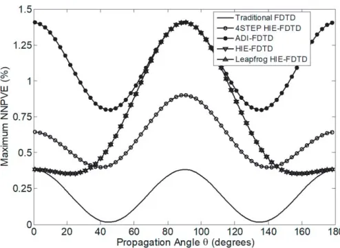
Figure 1. Maximum normalized numerical phase velocity error (NNPVE) versusθ with CFLN = 1.2, CPW = 15 and Δx= Δy= Δzfor the five FDTD methods. (Notice that the maximum NNPVE is the same between HIE-FDTD and leapfrog HIE-FDTD).

than that of the ADI-FDTD method and less than those of the other two HIE-FDTD methods when θ is between 36◦ and 144◦. Furthermore, it is noticed that the maximum NNPVE of the HIE-FDTD method is consistent with that of the one-step leapfrog HIE-FDTD method.

Fig. 2 shows the maximum NNPVE versusθwith CFLN = 3.6, CPW = 15 and Δx= Δz= 5Δyfor the five FDTD methods in the nonuniform grid system. From Fig. 2, it can be seen that the maximum NNPVE of the proposed method is significantly lower than that of the ADI-FDTD method, and this result is similar to that in the uniform grid system. Moreover, the maximum NNPVE of the proposed method is slightly lower than those of the other two HIE-FDTD methods, whenθ is between 40◦ and 140◦.

Figure 2. Maximum NNPVE versus θ with CFLN = 3.6, CPW = 15 and Δx = Δz = 5Δy for the five FDTD methods. (Notice that the maximum NNPVE is the same between HIE-FDTD and leapfrog HIE-FDTD).

Figure 3. Maximum NNPVE versusθwith CPW = 15 and Δx= Δz= (Δy,2Δy,5Δy,10Δy) for the proposed method.

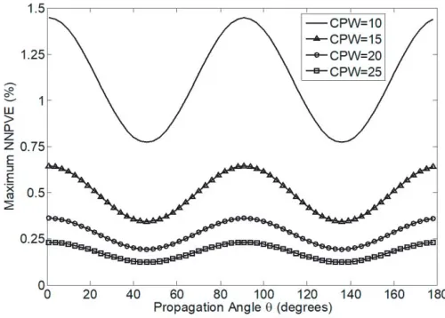
Figure 4. Maximum NNPVE versusθwith CFLN = 3.6, CPW = (10, 15, 20, 25) and Δx= Δz= 5Δy for the proposed method.

the proposed method with different CPW values. As shown in Fig. 4, it is clear that the maximum NNPVE of the proposed method decreases when the CPW value increases. It can be inferred that the maximum NNPVE of the proposed method can be reduced by adopting the fine grid.

5. NUMERICAL RESULTS

at 4.2 mm away from the central point in the x-direction, and the total simulation time is selected to be 5.7735 ns.

Figure 5 shows theEx-field for the five FDTD methods at the observation point with Δx= Δz=

5Δy = 0.6 mm and CFLN = 1 for the traditional FDTD method, CFLN = 3 for other four FDTD methods. From Fig. 5, it can be demonstrated that the result of the proposed method agrees well with that of the traditional FDTD method.

Figure 5. Ex-field for the five FDTD methods with Δx= Δz= 5Δy= 0.6 mm and CFLN = 1 for the

traditional FDTD method, CFLN = 3 for other FDTD methods.

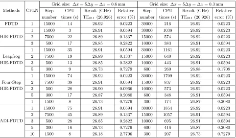
Table 1. The comparisons of the simulation results of the five FDTD methods using the coarse and the fine grid.

Methods CFLN

Grid size: Δx= 5Δy= Δz= 0.6 mm Grid size: Δx= 5Δy= Δz= 0.3 mm Step

number

CPU times (s)

Result (GHz) TE011 (26.926)

Relative error (%)

Step number

CPU times (s)

Result (GHz) TE011 (26.926)

Relative error (%)

FDTD 1 15000 14 26.92 0.0223 30000 216 26.92 0.0223

HIE-FDTD

1 15000 3 26.91 0.0594 30000 1038 26.92 0.0223

2 7500 22 26.89 0.1337 15000 574 26.92 0.0223

3 500 17 26.85 0.2822 10000 383 26.91 0.0594

Leapfrog HIE-FDTD

1 15000 35 26.91 0.0594 30000 1161 26.92 0.0223

2 7500 19 26.89 0.1337 15000 640 26.92 0.0223

3 500 13 26.85 0.2822 10000 443 26.91 0.0594

5 300 9 26.73 0.7279 600 260 26.88 0.1708

Four-Step HIE-FDTD

1 15000 74 26.92 0.0223 30000 1709 26.92 0.0223

2 7500 38 26.91 0.0594 15000 837 26.92 0.0223

3 500 28 26.90 0.0966 10000 573 26.92 0.0223

5 300 17 26.87 0.2080 600 348 26.91 0.0594

1 1500 8 26.73 0.7279 300 174 26.87 0.2080

ADI-FDTD

1 15000 75 26.91 0.0594 30000 1854 26.92 0.0223

2 7500 45 26.89 0.1337 15000 1057 26.91 0.0594

3 500 28 26.85 0.2822 10000 695 26.91 0.0594

5 300 16 26.73 0.7279 600 416 26.87 0.2080

Table 1 indicates the comparisons of the simulation results of the five FDTD methods by using the coarse grid Δx= Δz = 5Δy = 0.6 mm and fine grid Δx= Δz = 5Δy = 0.3 mm with different CFLN values, respectively. For the fine grid and CFLN = 10, a comparison of the proposed method and ADI-FDTD method shows that the former method improves the computational accuracy from 0.7279% to 0.2080% and reduces the CPU time from 207 s to 174 s. Consequently, with the better level of accuracy, the former method saves the CPU time by more than 15.9%. From the results mentioned above, it can be inferred that the proposed method is superior to the ADI-FDTD method in both the computational efficiency and accuracy.

Moreover, for the HIE-FDTD method, leapfrog HIE-FDTD method, and ADI-FDTD method with CFLN = 3, and for the proposed method with CFLN = 2, it can be seen from Table 1 that the proposed method using the coarse grid has the same level of computational accuracy as other three FDTD methods using the fine grid, but the CPU time is reduced from 383 s, 443 s, and 695 s of the HIE-FDTD method, leapfrog HIE-FDTD method, and ADI-FDTD method to 38 s of the proposed method. In other words, with the same level of accuracy, the proposed method can reduce the computational time by increasing the grid size, thus the efficiency of the proposed method is improved. Consequently, with the same level of accuracy, the proposed method has higher computational efficiency than other three FDTD methods.

6. CONCLUSION

A novel four-step HIE-FDTD method with weaker stability condition and higher computational efficiency in 3-D domains has been proposed in this paper. Based on the exponential evolution operator (EEO), the Maxwell’s equations are split into four sub-procedures first, and then the implicit scheme is applied only in one direction with the fine mesh; the explicit scheme is applied in two other directions with the coarser mesh; and the formulation of the proposed method has been generated.

The CFL stability condition of the proposed method is more relaxed than those of existing HIE-FDTD methods. Besides, the maximum NNPVE of the proposed method is less than that of the ADI-FDTD method obviously. Finally, the numerical experiments have demonstrated that the proposed method agrees very well with the traditional FDTD method. Compared with the ADI-FDTD method, the proposed method has a better level of accuracy and higher computational efficiency. Moreover, with the same level of computational accuracy, the proposed method has higher computational efficiency than those of the HIE-FDTD method, leapfrog HIE-FDTD method, and ADI-FDTD method. Therefore, the four-step HIE-FDTD method can be used for solving electromagnetic field problems with fine structures in one direction with higher computational efficiency. In addition, extending the proposed method into the dispersive media and applying it to solve some electromagnetic problems, such as the waveguide, antenna, and electromagnetic compatability (EMC) problems, will be our future work.

ACKNOWLEDGMENT

This work was supported by the National Natural Science Foundation of China under Grant 61671207 and the Fundamental Research Funds for the Central Universities (2015ZM066 and 2017ZD055).

REFERENCES

1. Yee, K. S., “Numerical solution of initial boundary value problems involving Maxwell’s equations in isotropic media,”IEEE Trans. Antennas Propag., Vol. 14, No. 3, 302–307, May 1966.

2. Taflove, A. and S. C. Hagness, Computational Electrodynamics: The Finite-Difference Time-Domain Method, 2nd Edition, Artech House, Boston, MA, 2000.

3. Namiki, T., “A new FDTD algorithm based on alternating-direction implicit method,”IEEE Trans. Microw. Theory Techn., Vol. 47, No. 10, 2003–2007, Oct. 1999.

5. Chen, J., Z. Wang, and Y. C. Chen, “Higher-order alternative direction implicit FDTD method,”

Electron. Lett., Vol. 38, No. 22, 1321–1322, Oct. 2002.

6. Fu, W. and E. L. Tan, “Stability and dispersion analysis for higher order 3-D ADI-FDTD method,”

IEEE Trans. Antennas Propag., Vol. 53, No. 11, 3691–3696, Nov. 2005.

7. Sun, G. and C. W. Trueman, “Efficient implementations of the Crank-Nicolson scheme for the finite-difference time-domain method,”IEEE Trans. Microw. Theory Techn., Vol. 54, No. 5, 2275– 2284, May 2006.

8. Tan, E. L., “Efficient algorithms for Crank-Nicolson-based finite difference time-domain methods,”

IEEE Trans. Microw. Theory Techn., Vol. 56, No. 2, 408–413, Feb. 2008.

9. Lee, J. and B. Fornberg, “A split step approaches for the 3-D Maxwell’s equations,” J. Comput. Appl., Vol. 158, 485–505, 2003.

10. Fu, W. and E. L. Tan, “Development of split-step FDTD method with higher-order spatial accuracy,” Electron. Lett., Vol. 40, No. 20, 1252–1253, Sep. 2004.

11. Chu, Q. X. and Y. D. Kong, “Three new unconditionally-stable FDTD methods with high-order accuracy,” IEEE Trans. Antennas Propag., Vol. 57, No. 9, 2675–2682, Sep. 2009.

12. Kong, Y. D. and Q. X. Chu, “High-order split-step unconditionally-stable FDTD methods and numerical analysis,”IEEE Trans. Antennas Propag., Vol. 59, No. 9, 3280–3289, Sep. 2011.

13. Shibayama, J., M. Muraki, J. Yamauchi, and H. Nakano, “Efficient implicit FDTD algorithm based on locally one-dimensional scheme,”Electron. Lett., Vol. 41, No. 19, 1046–1047, Sep. 2005.

14. Ahmed, I., E. Chua, E. P. Li, and Z. Chen, “Development of three-dimensional unconditionally stable LOD-FDTD method,” IEEE Trans. Antennas Propag., Vol. 56, No. 11, 3596–3600, Nov. 2008.

15. Saxena, A. K. and K. V. Srivastava, “A three-dimensional unconditionally stable five-step LOD-FDTD method,”IEEE Trans. Antennas Propag., Vol. 62, No. 3, 1321–1329, Mar. 2014.

16. Chen, J. and J. Wang, “A novel WCS-FDTD method with weakly conditional stability,” IEEE Trans. Electromagn. Compat., Vol. 49, No. 2, 419–426, May 2007.

17. Wang, J. B., B. H. Zhou, C. Gao, B. Chen, and L. H. Shi, “An efficient one-step leapfrog WCS-FDTD method,”IEEE Antennas Wireless Propag. Lett., Vol. 13, 1088–1091, 2014.

18. Huang, B. K., G. Wang, Y. S. Jiang, and W. B. Wang, “A hybrid implicit-explicit FDTD scheme with weakly conditional stability,” Microw. Opt. Technol. Lett., Vol. 39, No. 2, 97–101, Oct. 2003. 19. Chen, J. and J. Wang, “A 3D hybrid implicit-explicit FDTD scheme with weakly conditional

stability,” Microw. Opt. Technol. Lett., Vol. 48, 2291–2294, Nov. 2006.

20. Chen, J. and J. Wang, “Comparison between HIE-FDTD method and ADI-FDTD mehtod,”

Microw. Opt. Technol. Lett., Vol. 49, No. 5, 1001–1005, May 2007.

21. Chen, J. and J. Wang, “Numerical simulation using HIE-FDTD method to estimate various antennas with fine scale structures,” IEEE Trans. Antennas Propag., Vol. 55, No. 12, 3603–3612, Dec. 2007.

22. Chen, J. and J. Wang, “A three-dimensional semi-implicit FDTD scheme for calculation of shielding effectiveness of enclosure with thin slots,”IEEE Trans. Electromagn. Compat., Vol. 49, No. 2, 354– 360, Feb. 2007.

23. Zhang, Q., B. Zhou, and J. B. Wang, “A novel hybrid implicit-explicit FDTD algorithm with more relaxed stability condition,”IEEE Antennas Wireless Propag. Lett., Vol. 12, 1372–1375, 2013. 24. Zhang, Q. and B. H. Zhou, “A novel HIE-FDTD method with large time-step size,”IEEE Antennas

Propag. Magaz., Vol. 57, No. 2, 24–28, Apr. 2015.

25. Wang, J. B., B. H. Zhou, L. H. Shi, C. Gao, and B. Chen, “A novel 3-D HIE-FDTD method with one-step leapfrog scheme,” IEEE Trans. Microw. Theory Techn., Vol. 62, No. 6, 1275–1283, Jun. 2014.