Study of the Shielding Effectiveness of Double Rectangular
Enclosures with Apertures Excited by an Internal Source
Jian-Hong Hao, Lu-Hang Jiang*, Yan-Fei Gong, and Jie-Qing Fan
Abstract—An analytical formulation has been developed to evaluate the shielding effectiveness (SE) of two coplanar rectangular metallic enclosures with a circular aperture excited by an internal electric dipole source. The formulation consists of three parts: First, the near-field electromagnetic interference (EMI) of the electromagnetic leakage from the aperture is represented by the electric dipole in one enclosure. Then, the aperture equivalent magnetic and electric dipole moments are calculated according to the Bethe’s small aperture coupling theory. Finally, the electric field of the other enclosure is derived by using the equivalent magnetic dipole field, equivalent electric dipole field and the corresponding enclosure’s Green’s functions in the two fields. In this formulation, the electric field of the enclosure can be expressed as a function of the observation point, the aperture’s center point, source point, shape of the aperture and enclosure’s conductivity. The formulation then is employed to analyze the effect of the above factors on the SE. The analytical results have been successfully compared with the full-wave simulation software Computer Simulation Technology (CST) from 0.3∼2.4 GHz.
1. INTRODUCTION
Electromagnetic field coupling into a metallic enclosure through apertures has become an important issue in recent years. The shielding effectiveness (SE) of a mono-enclosure [1–3] or multiple enclosures [4– 6] with apertures has been especially studied by using numerical methods and analytical formulations. Numerical methods, including the finite difference time domain (FDTD) method [7, 8], finite element method (FEM) [9], method of moments (MoM) [10, 11], and transmission-line modeling (TLM) method [12], are robust and accurate but always require large computational resources. Analytical formulations such as the Bethe’s small aperture coupling theory [13–15], equivalent circuit method [1– 3, 16] and BLT equation [6, 17], although approximate, are much faster than numerical methods, and more convenient in investigating the effect of design parameters on the SE. The SE of a shielding enclosure is defined as the ratio of field strengths in the presence and absence of the enclosure.
The SE of double rectangular enclosures with apertures against an external plane wave is investigated in [4–6]. It is far-field electromagnetic interference (EMI), and the field source is placed outside the enclosure. However, there exist lots of situations in which the field source is required to be placed inside the enclosure. The electromagnetic leakage of an apertured rectangular enclosure excited by an internal electric dipole is studied in [15]. The electromagnetic field coupling with a transmission line located in a rectangular enclosure excited by an internal electric dipole is studied in [18]. In fact, with the rapid development of large-scale integrated circuit, the enclosure is always divided into several regions mainly to reduce the near-field EMI from electronic devices and components of adjacent enclosures through the apertures. Unlike far-field EMI, near-field EMI is more complex and destructive. Therefore, it is necessary to study the universal near-field EMI between adjacent enclosures.
In this paper, an analytical formulation has been developed to evaluate the SE of two coplanar rectangular metallic enclosures with a circular aperture excited by an internal electric dipole. First,
Received 25 January 2016, Accepted 21 March 2016, Scheduled 27 March 2016
* Corresponding author: Lu-Hang Jiang ([email protected]).
the near-field EMI of the electromagnetic leakage from the aperture is represented by the electric dipole in one enclosure. Then, the aperture equivalent magnetic and electric dipole moments are calculated according to the Bethe’s small aperture coupling theory. Finally, the electric field of the other enclosure is derived by using the equivalent magnetic dipole field, equivalent electric dipole field and the corresponding enclosure’s Green’s functions in the two fields. In [4], the rectangular aperture coupling with large length-width ratio is studied, and the aperture’s radiation can be represented only with the magnetic polarizability, considering the negligible contribution of the electric polarizability. In our model, both of the magnetic and electric polarizabilities are taken into consideration in order to study the circular aperture coupling. Therefore, the analytical formulation proposed is more accurate in most of the frequency band from 0.3∼2.4 GHz than the model in which only the magnetic polarizability is considered in evaluating the SE of the enclosure.
The rest of the paper is organized as follows. Section 2 presents the geometry and mathematical formulas of the analytical model. Section 3 illustrates the verification with a conventional full-wave simulation tool CST and analyzes the effect of some parameters of the enclosure on the SE. Finally, some conclusions are drawn in Section 4.
2. THEORY
2.1. Analytical Model
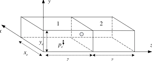
The geometry of the analytical model is shown in Figure 1. It consists of two coplanar rectangular metallic enclosures (enclosure 1 and enclosure 2) with a circular aperture on the planez=zeexcited by an electric dipole in enclosure 1. The dimensions of the enclosures are bothxe×ye×ze. The diameter of the aperture is d, and the center point of the aperture is located at P0(x0, y0, z0). The source
interference is an electric dipole oriented along they-axis located atPs(xs, ys, zs). The SE observation point is located at P(x, y, z) in enclosure 2.
x
y
z
e x
e y
e
z ze
e p
1 2
Figure 1. Double rectangular metallic enclosures with a circular aperture excited by an internal electric dipole.
According to the Bethe’s small aperture coupling theory, usually when the diameter of the circular aperture is shorter than 1/10 wavelength of interest, the leakage field of enclosure 2 can be represented by the aperture equivalent electric and magnetic dipole moments p and m[13]. The equations linking the dipole moments and the unperturbed fields of enclosure 1, when it is totally closed, are [15]
p = αezε0Eu,zez (1)
m = −αmxHu,xex−αmyHu,yey (2) where ε0 is the electric permittivity of vacuum; Eu,z is the unperturbed electric field along thez-axis;
Hu,x and Hu,y are the unperturbed magnetic field along the x-axis and y-axis, respectively; αez, αmx and αmy are the electric polarizability along the z-axis, magnetic polarizability along the x-axis and magnetic polarizability along the y-axis, respectively. The polarizability is dependent only upon the shape and size of the aperture.
For a circular aperture with diameterd, the polarizability is [19]
Eu,z,Hu,x and Hu,y are given by [15]
Eu,z = k−jωμ2(x 0Idl
eyeze) ∞ n=0 ∞ l=0 Γnl y e 2
× {sink1[ye−(y0+ys)] + sgn (y0−ys) sink1(ye− |y0− ys|)} ×sin (k1ye)−1 (4)
Hu,x = (−Idl xeyeze)
∞ n=0 ∞ l=0 Γnl ye 2k1
×[cosk1(y0+ys−ye) + cosk1(|y0− ys| −ye)]×sin (k1ye)−1 (5)
Hu,y = 0 (6)
where ω = 2πf; μ0 is the magnetic permeability of vacuum; k is the free space wavenumber; I and dl
are the current and length of the electric dipole, respectively; nand l are the field mode number along thex-axis and z-axis, respectively.
k1 =
k2−(nπx
e)2−(lπz
e)2 (7)
Γnl = ε0nε0l lπ ze cos lπz0 ze sin lπzs ze sin nπx0 xe sin nπxs xe (8)
whereε0n and ε0l are Neumann factors,ε0n(l)= 1 for n(l) = 0 andε0n(l)= 2 for n(l)= 0.
2.2. Electric Field and SE Calculation for the Magnetic Polarizability
When the equivalent magnetic dipole moment is considered, enclosure 2’s Green’s function is presented as follows [14]:
Gm = − ∞ n=0 ∞ m=0
ε0nε0m
xeye
sin(kxx0) cos(kyy0)
knmsin(knmze)
sin(kxx) cos(kyy)
× {cos [knm(|z+z0| −ze)] + cos [knm(|z−z0| −ze)]} (9)
where ε0m is Neumann factor, ε0m = 1 for m= 0 and ε0m = 2 for m = 0. kx =nπ/xe, ky = mπ/ye,
knm =
k2−k2
x−ky2. m is the field mode number along they-axis. The electric fieldE is related toGm as follows:
E=−jωμ0αmxHu,x(∇ ×Gm) (10)
Substituting Eq. (9) into Eq. (10), the electric field components of enclosure 2 may be derived as follows:
Emx = 0 (11)
Emy = −jωμ0αmxHu,x
∞ n=0 ∞ m=0
ε0nε0m
xeye
sin(kxx0) cos(kyy0)
sin(knmze)
sin(kxx) cos(kyy)
× {sin [knm(ze− |z+z0|)] + sgn(z−z0) sin [knm(ze− |z−z0|)]} (12)
Emz = −jωμ0αmxHu,x
∞ n=0 ∞ m=0
ε0nε0m
xeye
ky sin(kxx0) cos(kyy0) knmsin(knmze)
sin(kxx) sin(kyy)
× {cos [knm(|z+z0| −ze)] + cos [knm(|z−z0| −ze)]} (13)
We can therefore calculate the SE for the magnetic polarizability at observation point P by superposition of the electric field components.
Em =
E2
mx+Emy2 +Emz2 (14)
SEm = −20 log10
|Em| |E0|
(15)
2.3. Electric Field and SE Calculation for the Electric Polarizability
Similarly, when the equivalent electric dipole moment is considered, enclosure 2’s Green’s function is presented as follows:
Ge = ∞ n=0 ∞ m=0 ∞ l=0 c2 xeyeze
cos(kxx0) cos(kyy0) sin(kzz0)
ω2
nml−ω2
cos(kxx) cos(kyy) sin(kzz) (16)
wherec is the velocity of light of vacuum,kz =lπ/ze,ωnml=
k2
x+k2y+k2z−k2
c2.
Equation (16) is a triple series. In order to improve its convergence rate, it is simplified as Equation (18) by using identical Equation (17)
∞
n=1
cosnx n2−a2 =
1 2a2 −
π 2a2
cos(x−n)a
sinπa (0≤x≤2π) (17)
Ge = ∞ n=0 ∞ m=0
ε0nε0m
xeye
cos(kxx0) cos(kyy0)
knmsin(knmze)
cos(kxx) cos(kyy)
× {cos [knm(|z+z0| −ze)]−cos [knm(|z−z0| −ze)]} (18)
The electric fieldE is related toGe as follows:
E=−(jωαeε0Eu,z)× (1/jωμ0ε0)∇
ε0∂Ge
∂z
−jωε0Geez
(19)
Substituting Eq. (18) into Eq. (19), the electric field components of enclosure 2 may be derived as follows:
Eex = −(jωαeε0Eu,z)
1 jωμ0 ∞ n=0 ∞ m=0
ε0nε0m
xeye
kx cos(ksin(xx0) cos(kyy0) knmze)
sin(kxx) cos(kyy)
× {sin [knm(ze− |z+z0|)]−sgn(z−z0) sin [knm(ze− |z−z0|)]} (20)
Eey = −(jωαeε0Eu,z)
1 jωμ0 ∞ n=0 ∞ m=0
ε0nε0m
xeye
ky cos(ksin(xx0) cos(kyy0) knmze)
cos(kxx) sin(kyy)
× {sin [knm(ze− |z+z0|)]−sgn(z−z0) sin [knm(ze− |z−z0|)]} (21)
Eez = −(jωαeε0Eu,z)
1 jωμ0 ∞ n=0 ∞ m=0
ε0nε0m
xeye
knm cos(ksin(xx0) cos(kyy0) knmze)
cos(kxx) cos(kyy)
× {cos [knm(z+z0−ze)] + cos [knm(|z−z0| −ze)]} (22)
We can therefore calculate the SE for the electric polarizability at observation point P by superposition of the electric field components.
Ee =
E2
ex+Eey2 +E2ez (23)
SEe = −20 log10
|Ee| |E0|
(24)
2.4. Electric Field and SE Calculation for Both of the Magnetic and Electric Polarizabilities
We can therefore calculate the total electric field components by superposition of Em components and Ee components
Finally, we can calculate the total SE at the observation point by superposition of the total electric field components
E =
E2
x+Ey2+Ez2 (26)
SE = −20 log10
|E| |E0|
(27)
3. RESULTS AND DISCUSSIONS
In this section, the SE of the observation point is calculated by using the analytical model proposed in Section 2. Various configurations including different positions of the observation point, aperture’s center point and electric dipole, different shapes of the aperture, and different conductivities of the enclosure are studied. So for verifying it, our results are compared with the CST simulation results in the frequency range 0.3 ∼2.4 GHz. It is important to notice that the electric dipole is oriented along they-axis in our model, so only the electric field along they-axis and the magnetic field along thex-axis have been considered in calculating the SE.
In Section 3.1, the SE for the magnetic polarizability, the SE for the electric polarizability, and the total SE for both of the magnetic and electric polarizabilities are calculated, respectively. The dimensions of the double enclosures are both 300 mm×120 mm×300 mm. The aperture radius is r = 5 mm. The aperture’s center point is located at P0 (150, 60, 300) mm. The electric dipole
and observation point are located at Ps (150, 60, 20) mm and P (150, 60, 450) mm, respectively. In Section 3.2, the effect of various parameters of the enclosure on the SE is analyzed.
3.1. Model Validation
Figure 2, Figure 3 and Figure 4 show the calculated SE for the magnetic polarizability, the SE for the electric polarizability and the total SE for both of the magnetic and electric polarizabilities respectively using the analytical model and the results from the CST. It can be seen that three resonant modes, TE101, TE301 and TE303, have been identified corresponding to the enclosure resonant frequencies,
0.71 GHz, 1.58 GHz and 2.12 GHz, respectively. Figure 5 shows the comparison of the calculated SE for the magnetic polarizability, electric polarizability and both of the magnetic and electric polarizabilities. In comparison of Figures 2, 3, 4 and 5, it can be seen that the result of Figure 4 is more accurate than that of Figure 2 and Figure 3 from 0.3∼2.12 GHz, and the result of Figure 2 is more accurate than that
0.3 0.6 0.9 1.2 1.5 1.8 2.1 2.4 -90
-60 -30 0 30 60 90 120 150 180
SE/dB
f/GHz CST
magnetic dipole
Figure 2. Calculated SE for the magnetic polarizability using the analytical model and the result from CST.
0.3 0.6 0.9 1 .2 1.5 1.8 2.1 2 .4 -90
-60 -30 0 30 60 90 120 150 180
SE
/d
B
f/GHz
CST
electric dipole
0.3 0.6 0.9 1.2 1.5 1.8 2.1 2.4 -90
-60 -30 0 30 60 90 120 150 180
SE/d
B
f/GHz
CST
magnetic and electric dipole
Figure 4. Calculated total SE for both of the magnetic and electric polarizabilities using the analytical model and the result from CST.
0.3 0.6 0.9 1.2 1.5 1.8 2.1 2.4 30
40 50 60 70 80 90 100 110 120
SE/d
B
f /GHz
magnetic dipole
magnetic and electric dipole electric dipole
Figure 5. Calculated SE for the magnetic polarizability, the electric polarizability and both of the magnetic and electric polarizabilities.
of Figure 3 and Figure 4 from 2.12∼2.4 GHz. Therefore, it is better to consider both of the magnetic and electric polarizabilities under 2.12 GHz.
3.2. The Effect of Various Parameters on the SE
By keeping the position of the electric dipole and the aperture’s center point unvaried, Figure 6 shows the calculated SE for different observation points of (150, 60, 450) mm, (202, 60, 450) mm and (228, 60, 450) mm. It can be seen that the nearer the observation point is to the side wall, the higher the SE will be. It is because wheny and zof the observation point are unvaried, while xchanges, the electric field depends on the function |sin (nπx/xe)|. If mode nis odd, |sin (nπx/xe)| decreases monotonically with the increase of independent variablex on the interval [150, 300] mm. The variation of the SE is similar forx on the interval [0, 150] mm, considering the symmetry of the double enclosures about the electric dipole and the aperture. Therefore, the nearer the observation point is to the side wall, the lower the
0.3 0.6 0.9 1.2 1.5 1.8 2.1 2.4 20
40 60 80 100 120
SE/
d
B
f/GHz
(150,60,450) (202,60,450) (228,60,450)
Figure 6. Calculated SE for different observation points withP0(x0, y0, z0) = (150, 60, 300) mm and
Ps(xs, ys, zs) = (150, 60, 20) mm.
0.3 0.6 0.9 1.2 1.5 1.8 2.1 .2.4 20
40 60 80 100 120
SE/d
B
f/GHz
(98,60,450) (150,60,450) (254,60,450)
0.3 0.6 0.9 1.2 1.5 1.8 2.1 2.4 20
40 60 80 100 120
SE/d
B
(150,40,150) (150,75,150) (150,100,150)
f/GHz
Figure 8. Calculated SE for different positions of the electric dipole with P0(x0, y0, z0) = (150, 60,
300) mm andP(x, y, z) = (150, 60, 450) mm.
electric field will be, and the higher the SE will be.
By keeping the position of the electric dipole unvaried, Figure 7 shows the calculated SE for different aperture’s center points of (150, 60, 300) mm, (98, 60, 300) mm and (254, 60, 300) mm. In order to keep the observation points on the central axis of the aperture, they are set at (150, 60, 450) mm, (98, 60, 450) mm and (254, 60, 450) mm, respectively. It can be seen that before the second resonant point, the nearer the aperture’s center point is to the side wall, the higher the SE will be. However, that law is not obvious after the second resonant point. In addition, the frequency points where the SE increases rapidly differ in the three graphs. The reason is that the aperture is at zero points of the electric field of the enclosure, which will change for different aperture’s center points.
By keeping the aperture’s center point atP0 (150, 60, 300) mm and the observation point atP (150,
60, 450) mm, Figure 8 shows the calculated SE for different electric dipole positions of (150, 40, 150) mm, (150, 75, 150) mm and (150, 100, 150) mm. It can be seen that the SE remains almost the same except in the frequency range at the very beginning. It is because according to Equations (4) and (5), the change of the independent variableysof the electric dipole contributes little to the unperturbed electric field componentEu,zand the unperturbed magnetic field componentHu,x. Therefore, the graphs almost keep the same in general.
By changing the polarizability of the aperture, Figure 9 shows the calculated SE for the rectangular aperture using the analytical model and the result from CST. It can be seen that the result from the analytical model is in good agreement with that from CST in most of the frequency band from 0.3∼2.4 GHz. Figure 10 shows the comparison of the calculated SE for the rectangular aperture and the circular aperture with the same size. It can be seen that the SE of the circular aperture increases about 15 dB compared with that of the rectangular aperture.
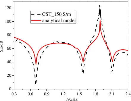
The material of the enclosure is perfect conductor in the above model. Next, the effect of the lossy material on the SE of the enclosure will be investigated. It is assumed that only the incident TEnmwave will be considered in the following research. For a rectangular enclosure, the propagation constants γ1
and γnm are presented as follows [3]:
γ1 =
−β2
0−(1−j)δ
ε0n
xe
kc20+β02
k2
x k2
c0
+ε0m ye
k2c0+β02
k2
y k2
c0
(28)
γnm =
−β2
0−(1−j)δ
ε0n
xe
kc20+β02
k2
x kc20
+ε0l ze
kc20+β02
k2
z kc20
(29)
wherekc0 =
k2
x+ky2 is the cutoff wavenumber of the TEnm mode; β0 =
k2−k2
c0,δ =
0.3 0.6 0.9 1.2 1.5 1.8 2.1 2.4 -100
-50 0 50 100 150
SE/dB
f/GHz
CST_rectangle model_rectangle
Figure 9. Calculated SE for the rectangular aperture using the analytical model and the result from CST.
0.3 0.6 0.9 1.2 1.5 1.8 2.1 2.4 20
40 60 80 100 120
SE
/d
B
f/GHz
model_circle model_rectangle
Figure 10. Calculated SE for circular aperture and rectangular aperture with the same size.
0.3 0.6 0.9 1.2 1.5 1.8 2.1 2.4 0
20 40 60 80 100 120
SE
/d
B
f/GHz
CST_60 S/m analytical model
Figure 11. Calculated SE when the enclosure 1 is perfect and the enclosure 2 is lossy with the conductivity of 60 S/m using the analytical model and the result from CST.
0.3 0.6 0.9 1.2 1.5 1.8 2.1 2.4 0
20 40 60 80 100 120
SE
/d
B
f/GHz
CST_150 S/m analytical model
Figure 12. Calculated SE when the enclosure 1 and enclosure 2 are both lossy with the conductivity of 150 S/m using the analytical model and the result from CST.
material, respectively. The electric field of the lossy enclosure can then be derived by the substitution of the parameters k1 and knm for the perfect enclosure [3].
k1=−jγ1, knm=−jγnm (30)
4. CONCLUSION
An analytical formulation has been developed to evaluate the SE of two coplanar rectangular metallic enclosures with a circular aperture excited by an internal electric dipole source. The electric field components of the observation points are derived according to the Bethe’s small aperture coupling theory and the enclosure’s Green’s function. The results from the analytical model are in good agreement with those from the full-wave simulation software CST in most of the frequency band from 0.3∼2.4 GHz. The results show that the observation point, aperture’s center point, shape of the aperture, and enclosure’s conductivity can all have a significant influence on the SE except the electric dipole source point. It is relatively fast, accurate and convenient to evaluate the SE and analyze the effect of different factors on it by using the analytical formulation proposed in comparison with numerical methods. The results are helpful for guiding the design of more complex electromagnetic shielding enclosures.
ACKNOWLEDGMENT
The authors thank for the funding support from the National Natural Science Foundation (No. 61372050).
REFERENCES
1. Shim, J., D. G. Kam, J. H. Kwon, and J. Kim, “Circuital modeling and measurement of shielding effectiveness against oblique incident plane wave on apertures in multiple sides of rectangular enclosure,” IEEE Trans. Electromagn. Compat., Vol. 52, No. 3, 566–577, 2010.
2. Hao, J.-H., P.-H. Qi, J.-Q. Fan, and Y.-Q. Guo, “Analysis of shielding effectiveness of enclosures with apertures and inner windows with TLM,”Progress In Electromagnetic Research M, Vol. 32, 73–82, 2013.
3. Jiao, C.-Q. and H.-Z. Zhu, “Resonance suppression and electromagnetic shielding effectiveness improvement of an apertured rectangular cavity by using wall losses,”Chin. Phys .B, Vol. 22, No. 8, 1–6, 2013.
4. Song, H., D.-F. Zhou, D.-T. Hou, T. Hu, and J.-Y. Lin, “Hybrid algorithm for slot coupling of double layer shielding cavity,” High Power Laser and Particle Beams, Vol. 20, No. 11, 1892–1898, 2008.
5. Hao, C. and D.-H. Li, “Shielding effectiveness of double-deck cavity with apertures,” Chinese Journal of Radio Science, Vol. 29, No. 1, 114–121, 2014.
6. Luo, J.-W., P.-A. Du, D. Ren, and P. Xiao, “BLT equation-based approach for calculating shielding effectiveness of double layer rectangular enclosures with apertures,”High Power Laser and Particle Beams, Vol. 27, No. 11, 1–6, 2015.
7. Liu, Q.-F., W.-Y. Yin, M.-F. Xue, J.-F. Mao, and Q.-H. Liu, “Shielding characterization of metallic enclosures with multiple slots and a thin-wire antenna loaded: multiple oblique EMP incidences with arbitrary polarizations,” IEEE Trans. Electromagn. Compat., Vol. 51, No. 2, 284–292, 2009. 8. Liu, Q.-F., W.-Y. Yin, J.-F. Mao, and Z.-Z. Chen, “Accurate characterization of shielding
effectiveness of metallic enclosures with thin wires and thin slots,” IEEE Trans. Electromagn. Compat., Vol. 51, No. 2, 293–300, 2009.
9. Shi, Z. and P.-A. Du, “Numerical simulation of near field shielding properties for aperture arrays based on FEM,”Chin. J. Electron., Vol. 37, No. 3, 634–639, 2009.
10. Khorrami, M. A., P. Dehkhoda, R. M. Mazandaran, and S. H. H. Sadeghi, “Fast shielding effectiveness calculation of metallic enclosures with apertures using a multiresolution method of moments technique,” IEEE Trans. Electromagn. Compat., Vol. 52, No. 1, 230–235, 2010.
12. Nie, B.-L., P.-A. Du, Y.-T. Yu, and Z. Shi, “Study of the shielding properties of enclosures with apertures at higher frequencies using the transmission-line modeling method,” IEEE Trans. Electromagn. Compat., Vol. 53, No. 1, 73–81, 2011.
13. Bethe, H. A., “Theory of diffraction by small apertures,” Physical Review Second Series, Vol. 66, 163–182, 1944.
14. Rao, Y.-P., H. Song, and D.-F. Zhou, “Fast estimation of shielding efficiency of cavity with thin slots,”High Power Laser and Particle Beams, Vol. 20, No. 8, 1327–1332, 2008.
15. Li, Y. Y. and C. Q. Jiao, “Analytical formulation for electromagnetic leakage from an apertured rectangular cavity,” PIERS Proceedings, 257–261, Guangzhou, China, Aug. 25–28, 2014.
16. Liu, E.-B., P.-A. Du, and B.-L. Nie, “An extended analytical formulation for fast prediction of shielding effectiveness of an enclosure at different observation points with an off-axis aperture,” IEEE Trans. Electromagn. Compat., Vol. 56, No. 3, 589–598, 2014.
17. Luo, J.-W., P.-A. Du, D. Ren, and B.-L. Nie, “A BLT equation-based approach for calculating the shielding effectiveness of enclosures with apertures,”Acta Phys. Sin., Vol. 64, No. 1, 1–8, 2015. 18. Boutar, A., A. Reineix, C. Guiffaut, and G. Andrieu, “An efficient analytical method for
electromagnetic field to transmission line coupling into a rectangular enclosure excited by an internal source,” IEEE Trans. Electromagn. Compat., Vol. 57, No. 3, 565–573, 2015.