Analysis of a Non-Integer Dimensional Tunnel and Perfect Electric
Conductor Waveguide
Nayab Bhatti and Qaisar A. Naqvi*
Abstract—Solutions to the Maxwell equations for a planar non-integer dimensional perfect electric conductor (NID-PEC) waveguide are obtained. The space within the guide is NID in direction normal to walls of the waveguide. Field behavior within the waveguide is noted for different values of the parameter, D, describing dimension of the NID space. For D= 2, classical results are recorded. The discussion is further extended by treating propagation in a tunnel within unbounded dielectric medium. The space within tunnel is also NID in direction perpendicular to walls of the tunnel. For different values of D field behaviors are also presented. It has been noted that for D= 2 and taking very high values of permittivity ( → ∞) classical results for PEC waveguide are recorded, whereas for → ∞, field behavior within tunnel matches with NID-PEC waveguide.
1. INTRODUCTION
In scientific literature term fractal is used to describe property of auto resemblance on all scales. This term was first coined by Mandelbrot to identify an object that is broken in space or time [1]. One of the intriguing interests of studying fractal is its capacity to model objects with complex structures [2]. Fractal dimension tells how the fractal is confined in the Euclidean space or how it fills the space in which it lies. Fractional order integrals may be used to describe the properties of fractal medium, and fractal medium behaves as continuous medium in non-integer dimensional (NID) space [3]. Consequently continuum models with NID space enable us to model and explain the behavior of fractal medium.
In 1977, Stillinger introduced the concept of NID space and proposed a mathematical basis for this subject and provided expression for generalized Laplace operator [4]. Later on, Palmer and Stavrinou [5] derived equations of motion for NID space. After these valuable initial contributions, the concept of NID space gained attention of researchers and now being used in various subjects of engineering and science [6]. For example, state of atomic bound was explained by the solution of Schrodinger equation [7]. Fractal theory of heterogeneous surfaces [8], Gauss’s law [9], Lagrangian formulation for field systems [10] had also been addressed in non-integer dimensional space. Solutions of Helmholtz’s equation were derived in unbounded NID space for cartesian [11], cylindrical [12] and spherical coordinates [13]. Solutions of Laplaces’s equation for cylindrical coordinates were derived in [14]. Quasi-static analysis of a plasmonic sphere [15], radiation from a two-dimensional buried canonical source [16], scattering from a low contrast buried cylinder [17], and buried strip [18] had also been treated when being immersed in NID space. Sadallah et al. proposed a solution of Euler-Lagrange equation in NID space [19]. Solution to the Maxwell’s equations inside the NID waveguide/transmission line was studied in [20]. Tarasov discussed Gauss’ law, Ampere’s law, and Poisson’s equation for fractal medium [21]. He proposed vector calculus for NID space, i.e., expressions for gradient, divergence, and Laplacian operator were given [22]. He also derived solutions for Poisson’s equation for fractal medium, Euler-Bernoulli fractal beam, and Timoshenko beam equations for fractal material [23]. Reflection and transmission from a
Received 16 January 2018, Accepted 28 February 2018, Scheduled 13 March 2018
* Corresponding author: Qaisar Abbas Naqvi ([email protected]).
planar interface of two non-integer dimensional half spaces were investigated in [24, 27]. Study of fractal continuum electromagnetics on the basis of three-dimensional continuum fractal metric was explained in [26].
In Cartesian coordinate, Laplacian and curl operator in non-integer dimensional space are defined in Appendix A. Maxwell curl equation and Helmholtz’s equation in D-dimensional space, for homogeneous and isotropic medium are given below,
∇D×E = −jωμH (1a)
∇D×H = jωE (1b)
∇2
DE+k2E = 0 (1c)
where k = ω√μ is the wave number. Time dependency exp(jωt) has been managed throughout the discussion.
In this paper, propagation of electromagnetic field in a NID-PEC waveguide and NID tunnel in dielectric medium has been treated one by one. For very high value of permittivity of the dielectric medium hosting the tunnel withD= 2, field behavior matches with the classical PEC waveguide result. For the sake of comparison, first, propagation of TE and TM modes in a PEC parallel plate waveguide is presented.
2. TE/TM-MODE IN PEC WAVEGUIDE
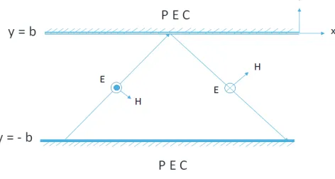
Consider a parallel plate PEC waveguide as shown in Figure 1. Two interfaces of the waveguide are located aty=±b. The medium inside the waveguide is described by the constitutive parametersand
μ. Suppose that transverse electric (TE) (Ex = 0) mode is propagating inside the waveguide. Field inside the waveguide is written as linear combination of two uniform plane waves. Electric and magnetic fields inside the waveguide are written below
Ez = Anexp(−jβx+jhy) +RAnexp(−jβx−jhy)
ηHx = −h
kAnexp(−jβx)[exp(jhy)−Rexp(−jhy)] ηHy = −β
kAnexp(−jβx)[exp(jhy) +Rexp(−jhy)]
whereR is the reflection co-efficient. It may be noted that k±=βxˆ∓hyˆare the two wave vectors.
Figure 1. TE mode in PEC waveguide.
By applying boundary conditions and substituting the values of unknown, the total electric field and magnetic field inside the waveguide may be written as,
Ez = Anexp(−jβx) sin{h(b−y)} (2a)
ηHx = −hkAnexp(−jβx) cos{h(b−y)} (2b)
ηHy = −β
whereh=nπ/2b.
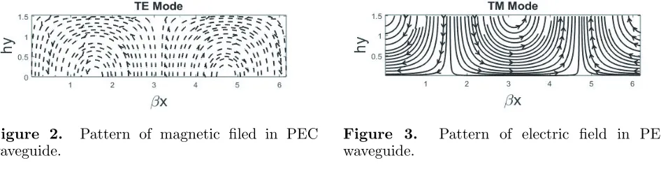
By using above set of equations, patterns of magnetic field lines are obtained as shown in Figure 2 which shows that magnetic field is tangential to the wall of the guide located athy = 1.5.
In order to examine the field behavior within PEC waveguide in xy-plane, here,θ1 =π/6 so that
β/k= cos(π/6), h/k= sin(π/6) are taken for the plot. In Figure 2, magnetic field lines become parallel to the walls of waveguide which shows that the walls are PEC, and the mode is transverse electric. Here, plot is considered for region 0≤y ≤b. It may be noted that symmetry exists for region −b≤y≤0.
Now, suppose that transverse magnetic (TM) (Hx= 0) mode is propagating inside the waveguide. Field inside the waveguide is written as linear combination of two uniform plane waves. The total electric and magnetic field inside the waveguide may be written as,
Ex = h
kAnexp(−jβx) sin{h(b−y)} (3a) Ey = βkAnexp(−jβx) cos{h(b−y)} (3b)
ηHz = Anexp(−jβx) cos{h(b−y)} (3c) By using Eq. (4), patterns of electric field are obtained as shown in Figure 3. It is obvious to note that electric field is normal to the wall of the guide located athy = 1.5.
Figure 2. Pattern of magnetic filed in PEC waveguide.
Figure 3. Pattern of electric field in PEC waveguide.
In Figure 3, electric field lines are perpendicular to the walls of waveguide which shows that the walls are PEC, and the mode is transverse magnetic. Here, again plot is considered for region 0 ≤y ≤+b. The field lines repeat themselves for every change of 2π (rad) in βx. In the remaining part of the discussion NID space will be taken into account, and the result given in the Section 2 will be used for comparison.
3. NID-PEC WAVEGUIDE
Consider a parallel plate PEC waveguide as shown in Figure 1. Two interfaces of the waveguide are located aty=±b. The medium inside the waveguide is described by the constitutive parametersand
μ. It has also been assumed that medium inside the waveguide is NID in direction normal to the walls of the waveguide.
Suppose that transverse electric (TE) (Ex = 0) mode is propagating inside the waveguide. Field inside the waveguide is written as linear combination of two waves propagating towards and away from each interface. These two waves are written below.
E1z = An
2 exp(−jβx)(hy) nH(1)
n (hy)
E2z = An
2 Rexp(−jβx)(hy) nH(2)
n (hy)
E1z is propagating in the +ve y direction whereasE2z is propagating in the−ve y direction. The total
electric field can be written as linear combination of above two waves, i.e.,
Ez = E1z+E2z
Ez = An
2 exp(−jβx)
(hy)nHn(1)(hy) +R(hy)nHn(2)(hy)
where Hn(1)(.) and Hn(2)(.) are the Hankel functions of the first and second kinds with the nth order,
n= 3−2D, 1< D≤2, andR is the unknown.
Corresponding magnetic field may be obtained using,
H = j
ωμ∇D ×E H = j
ωμ
∂ ∂yEz+
(α−1) 2y Ez−
∂ ∂zEy
ˆ
x−
∂ ∂xEz
ˆ
y+
∂ ∂xEy
ˆ
z
Substitutingα=D−1, above equation takes the following form,
H= j
ωμ
∂ ∂yEz+
(D−2) 2y Ez−
∂ ∂zEy
ˆ
x−
∂ ∂xEz
ˆ
y+
∂ ∂xEy
ˆ
z
As electric field contains onlyz-component,
ηH= j
k
∂ ∂yEz+
1 2
D−2
y Ez xˆ−
∂
∂xEz yˆ
where k = ω√μ is the wave number, and η = μ/ is the intrinsic impedance of the medium. Components of the magnetic field are,
ηHx = jh
k An
2 exp(−jβx)
(hy)nHnh(1)(hy) +R(hy)nHnh(2)(hy)
(4b)
ηHy = −β
k An
2 exp(−jβx)
(hy)nHn(1)(hy) +R(hy)nHn(2)(hy)
(4c)
where
H(1)
nh(hy) = Hn(1)−1(hy) +
1 2
D−2
hy Hn(1)(hy) H(2)
nh(hy) = Hn(2)−1(hy) +
1 2
D−2
hy Hn(2)(hy)
Applying boundary condition, unknown is obtained as,
R=−H
(1)
n (hb)
H(2)
n (hb)
(5)
Field expressions for electric and magnetic fields are,
Ez = An
2 exp(−jβx)
(hy)nHn(1)(hy)−H
(1)
n (hb)
H(2)
n (hb)
(hy)nHn(2)(hy)
(6a)
ηHx = jh
k An
2 exp(−jβx)
(hy)nHnh(1)(hy)−H
(1)
n (hb)
H(2)
n (hb)
(hy)nHnh(2)(hy)
(6b)
ηHy = −βkA2nexp(−jβx)
(hy)nHn(1)(hy)−H
(1)
n (hb)
H(2)
n (hb)
(hy)nHn(2)(hy)
(6c)
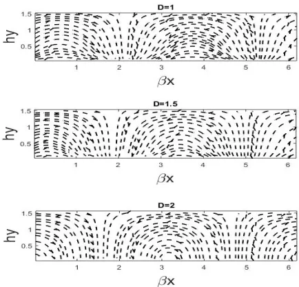
Using above set of equations, patterns of magnetic field for different values ofDare obtained as shown in Figure 4.
In order to examine the field behaviour within NID-PEC waveguide for different values ofDinxy -plane, here,θ1 =π/6 so thatβ/k= cos(π/6), h/k= sin(π/6) are taken for the plots. In all these plots,
Figure 4. Patterns of magnetic field for different values ofD.
4. PLANAR SLAB NID WAVEGUIDE
Consider a planar slab waveguide in unbounded dielectric medium as shown in Figure 5. The medium inside the slab is NID in direction normal to the interfaces of the slab. Two interfaces of the slab are located at y = ±b. The medium inside the slab is described by the constitutive parameters 1 and
μ. Host medium is dielectric, and its constitutive parameters are represented by 2 and μ. Suppose
that a TE wave (Ex = 0) is propagating inside the slab. The whole geometry has been divided into three regions so that the unknown fields can be written using the solution of homogeneous Helmholtz’s equation. Region y > b is titled as region I, −b < y < b titled as region II, and y <−b titled as region III. Non-integer dimension of medium is designated for region II isD.
Figure 5. NID tunnel in a dielectric medium.
Field inside the slab is written as linear combination of two uniform plane waves. The total electric and magnetic fields are given below
E2z = An
2 exp(−jβ1x)
(h1y)nHn(1)(h1y) +R(h1y)nHn(2)(h1y)
(7a)
obtained using the following Maxwell equation
∇D×E2=−jωμ1H2
Using above equation, the following may be obtained as
η1H2x = jhk1 1
An
2 exp(−jβ1x)
(h1y)nHnh(1)(h1y) +R(h1y)nHnh(2)(h1y)
(7b)
η1H2y = −β1
k1
An
2 exp(−jβ1x)
(h1y)nHn(1)(h1y) +R(h1y)nHn(2)(h1y)
(7c)
Field in region I is written below
E1z =T1An
2 exp(−jβ2x−jh2y) (8a)
Corresponding magnetic field may be obtained as
η2H1 =−T1An
2 1
k2
[h2xˆ−β2yˆ] exp(−jβ2x−jh2y) (8b)
Field in region III is written below
E3z =T2An
2 exp(−jβ1x+jh2y) (9a)
Corresponding magnetic field may be obtained as
η2H3=T2An
2 1
k2
[h2xˆ+β2yˆ] exp(−jβ2x+jh2y) (9b)
The unknown coefficients in the above expressions can be determined using the boundary conditions. At y = ±b, tangential components of electric and magnetic field must be continuous. Let field make an angle θ1 normal to the planar interfaces of the slab. The refraction angle θ2 can be determined by
using the following Ibn-Sahl’s law
k1sinθ1 =k2sinθ2
Application of boundary conditions yields
R=−
η1cosθ2Hn(1)(h1b) +jη2cosθ1Hnh(1)(h1b)
η1cosθ2Hn(2)(h1b) +jη2cosθ1Hnh(2)(h1b)
(10)
Plots represent patterns of magnetic field, for different values of2.
5. SPECIAL CASES
5.1. Case 1:
For 2 → ∞, planar slab NID waveguide converts into NID-PEC waveguide. The reflection coefficient
of Eq. (10) is transformed as,
R=−H
(1)
n (h1b)
H(2)
n (h1b)
Corresponding field expressions take the following forms,
E2z = An
2 exp(−jβ1x)
(h1y)nHn(1)(h1y)−H (1)
n (h1b)
H(2)
n (h1b)
(h1y)nHn(2)(h1y)
(11a)
η1H2x = −jhk1 1
An
2 exp(−jβ1x)
(h1y)nHnh(1)(h1y)−H (1)
n (h1b)
H(2)
n (h1b)
(h1y)nHnh(2)(h1y)
(11b)
η1H2y = −β1
k1
An
2 exp(−jβ1x)
(h1y)nHn(1)(h1y)−H (1)
n (h1b)
H(2)
n (h1b)
(h1y)nHn(2)(h1y)
(11c)
5.2. Case 2:
For2 → ∞,D= 2 yields R = exp(2jh1b).
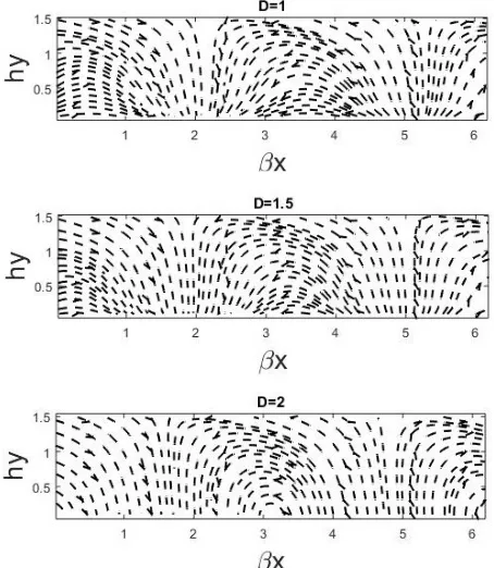
Figure 6. Patterns of magnetic field in NID tunnel (2 = 2).
Figure 7. Patterns of magnetic field in NID tunnel (2 = 4).
Figure 8. Patterns of magnetic field in NID tunnel (2 = 8).
This means that NID tunnel must behave as PEC waveguide.
In order to analyze the field behavior within NID tunnel, plots inxy plane are given taking different values of D and . It is obvious to note that as value of permittivity of the host medium increases, value of tangential component of the magnetic field increases at the walls of the tunnel. This behavior is depicted in Figure 6 to Figure 10. For very high values of the permittivity of host medium, the situation becomes the same as NID-PEC waveguide. In other words, normal component of magnetic field becomes zero at walls of the waveguide. So field lines are parallel to the walls. Keeping permittivity of the host medium constant, the variation in dimension has significant effects on the field pattern within the tunnel/waveguide.
Figure 10. Patterns of magnetic field in NID tunnel (2 = 1000).
6. CONCLUSION
Field expressions for electromagnetic mode propagating inside NID-PEC waveguide and NID tunnel for different values of D are derived. The field inside the waveguide and tunnel are written in terms of plane waves, and unknowns are determined by applying boundary conditions. Derived expressions are reduced to classical result when integer dimension is taken. In all the NID plots, effects of variation in the values of Dare very prominent.
APPENDIX A.
Laplacian operator for non-integer dimensional space having dimension D for cartesian coordinates is defined as [5]
∇2
D = ∂
2
∂x2 +
α1−1
x ∂ ∂x+
∂2
∂y2 +
α2−1
y ∂ ∂y+
∂2
∂z2 +
α3−1
z ∂
In NID space, curl operator for Cartesian coordinate is given below,
∇D×F(x, y, z) =
∂ ∂yFz+
1 2
α2−1
y Fz −
∂ ∂zFy+
1 2
α3−1
z Fy xˆ
+
∂ ∂zFx+
1 2
α3−1
z Fx −
∂ ∂xFz+
1 2
α1−1
x Fz yˆ
+
∂ ∂xFy +
1 2
α1−1
x Fy −
∂ ∂yFx+
1 2
α2−1
y Fx zˆ (A2)
whereF(x, y, z) is a vector function.
Following identities have been used to get the expressions for integer dimensional cases [25].
H(1)
−n = exp(jnπ)Hn(1)(hy) (A3)
H(2)
−n = exp(−jnπ)Hn(2)(hy) (A4)
H(1)
1
2 (hy) =
2
π
exp{j(hy−π2)} √
hy (A5)
H(1)
−1
2(hy) = j
2
π
exp{j(hy−π2)} √
hy (A6)
H(2)
1
2 (hy) =
2
π
exp{−j(hy−π2)} √
hy (A7)
H(2)
−1
2(hy) = −j
2
π
exp{−j(hy−π2)} √
hy (A8)
REFERENCES
1. 1 Mandelbrot, B. B. and J. W. V. Ness, “Fractional brownian motions, fractional noises and applications,” Vol. 10, No. 4, 422–437, 1968.
2. 2 Dimri, V. P. and R. P. Srivastava,Fractal Behaviour of the Earth System, 23–37, Springer Berlin Heidelberg, Hyderabad, 2005.
3. 3 Tarasov, V. E., “Continuous medium model for fractal media,” Physics Letters A, Vol. 336, 167–174, 2005.
4. 4 Stillinger, F. H., “Axiomatic basis for spaces with non-integer dimensions,” Journal of Mathematical Physics, Vol. 18, 1224–1234, 1977.
5. 5 Palmer, C. and P. N. Stavrinou, “Equations of motion in a non-integer-dimensional space,” Journal of Physics A, Vol. 37, 6987–7003, 2004.
6. 6 Zubair, M., M. J. Mughal, and Q. A. Naqvi, Electromagnetic Fields and Waves in Fractional Dimensional Space, Springer-Verlag, New York, 2012.
7. 7 Herrick, D. R. and F. H. Stillinger, “Variable dimensionality in atoms and its effects on the ground state of the helium isoelastic sequence,”Physical Review A, Vol. 11, 42–53, 1975.
8. 8 Pfeifer, P. and D. Avnir, “Chemistry in non-integer dimensions between two and three. I. Fractal theory of heterogeneous surfaces,”Journal of Chemical Physics, Vol. 79, 3558–3565, 1983.
9. 9 Muslih, S. I., M. Saddallah, D. Baleanu, and E. Rabei, “Lagrangian formulation of Maxwell’s field in fractional D dimensional space-time,” Romanian Journal of Physics, Vol. 55, 659–663, 2010. 10. Muslih, S. I., M. Saddallah, D. Baleanu, and E. Rabei, “Lagrangian formulation of Maxwell’s field
in fractional D dimensional space-time,” Romanian Reports of Physics, Vol. 55, 659–663, 2010. 11. Zubair, M., M. J. Mughal, and Q. A. Naqvi, “The wave equation and general plane wave solutions
in fractional space,” Progress In Electromagnetics Research Letters, Vol. 19, 137–146, 2010. 12. Zubair, M., M. J. Mughal, and Q. A. Naqvi, “An exact solution of the cylindrical wave equation
13. Zubair, M., M. J. Mughal, and Q. A. Naqvi, “An exact solution of the spherical wave equation in D-dimensional fractional space,” Journal of Electromagnetics Waves and Applications, Vol. 25, No. 10, 1481–1491, 2011.
14. Naqvi, Q. A. and M. Zubair, “On cylindrical model of electrostatic potential in fractional dimensional space,” Optik-International Journal for Light and Electron Optics, Vol. 127, 3243– 3247, 2016.
15. Noor, A., A. A. Syed, and Q. A. Naqvi, “Quasi-static analysis of scattering from a layered plasmonic sphere in fractional space,” Journal of Electromagnetic Wave and Applications, Vol. 29, No. 8, 1047–1059, 2015.
16. Munawar, Y., M. A. Ashraf, Q. A. Naqvi, and M. A. Fiaz, “Two dimensional green’s function for planar grounded dielectric layer in non-integer dimensional space,”Optik-International Journal for Light and Electron Optics, Vol. 140, 610–618, 2017.
17. Abbas, M., A. A. Rizvi, M. A. Fiaz, and Q. A. Naqvi, “Scattering of electromagnetic plane wave from a low contrast circular cylinder buried in non-integer dimensional half space,” Journal of Electromagnetic Waves and Applications, Vol. 31, No. 3, 263–283, 2017.
18. Naqvi, Q. A., “Scattering from a cylindrical obstacle buried in non-integer dimensional dielectric half space using kobayashi potential method,” Optik-International Journal for Light and Electron Optics, Vol. 141, 39–49, 2017.
19. Sadallah, M., S. I. Muslih, and D. Baleanu, “Equations of motion for Einstein’s field in non-integer dimensional space,”Czechoslovak Journal of Physics, Vol. 56, 323–328, 2006.
20. Khan, S. and M. J. Mughal, “General solution for TEM, TE, and TM waves in fractional dimensional space and its application in rectangular waveguide filled with fractional space,”Journal of Electromagnetic Waves and Applications, Vol. 27, No. 18, 2298–2307, 2013.
21. Tarasov, V. E., “Fractal electromagnetics via non-integer dimensional space approach,” Physics Letters A, Vol. 379, 2055–2061, 2015.
22. Tarasov, V. E., “Vector calculus in non-integer dimensional space and its applications to fractal media,”Journal of Communications in Nonlinear Science and Numerical Simulation, Vol. 21, No. 2, 360–374, 2015.
23. Tarasov, V. E., “Anisotropic fields media by vector calculus in non-integer dimensional space,” Journal of Mathematical Physics, Vol. 55, 083510, 2014.
24. Naqvi, Q. A. and M. A. Fiaz, “Electromagnetic behavior of a planar interface of non-integer dimensional spaces,” Journal of Electormagnetic Waves and Applications, Vol. 31, No. 16, 1625– 1637, 2017.
25. Abramowitz, M. and I. A. Stegun, Handbook of Mathematical Functions with Formulas, Graphs, and Mathematical Tables, U.S. Department of Commerce, 1972.
26. Balankin, A. S., B. Mena, J. Patino, and D. Morales, “Electromagnetic fields in fractional continua,” Physics Letter A, Vol. 377, 783–788, 2013.