Electrostatic Trap for Localisation and Confinement of Likely
Charged Particles
Ildar Tukaev*
Abstract—This paper reviews the motion of a charged particle in the electrostatic field of two coaxial likely charged rings located at some distance from one another. The charges of rings and that of the particle are of the same sign. Initial conditions of motion of the particle relatively to the rings under which the particle overcomes the electrostatic repulsion of rings and localises along a particular circular trajectory laying in the internal space between the rings were determined.
1. INTRODUCTION
We shall determine the term ring as a circle of the R0 radius with the linear density of electrostatic chargeQ/(2πR0). As of March 2016, known methods of localisation and confinement of charged particles in traps using the electrostatic fields are described in [1]. The principles of work of these traps and conditions under which particles are localised and confined there are considered in [2, 3]. The method of localisation and confinement of likely charged particles claimed in this paper is different from other known methods. Its principle is localisation of charged particles in the space between two coaxial electrostatic charged rings (charges of rings and those of particles are like). The electrostatic trap localises particles that have particular initial conditions of motion relatively to the rings; with these conditions, particles overcome the electrostatic repulsion of rings and localise along particular circular trajectories laying within the internal space between the rings. After the particles are localised, they may be confined for a long period of time. The advantage of the method claimed over known those is, first, that the localisation of particles can be performed in vacuum while the energy of particles is spent only for radiation, and second, that the localisation of particles can be performed in the continuous mode without changing the electrostatic field of rings; the latter allows to both localise and confine the charged particles simultaneously. The particles which initial conditions of motion do not match the localisation conditions are ejected from the system of rings.
Localisation of a particle and its confinement in the trap of the constant electrostatic field becomes possible when a force acting on the localising particle from the side of rings changes the direction of its action after it passes the zero value of its magnitude while the position of the particle relatively to the rings is changing — this is the property of intensity of the constant electrostatic field of two coaxial rings under particular conditions.
Therefore, the method claimed in this paper allows to single the particles having the kinetic energy of particular range out from the flow of likely charged those, localise and confine them. As the particles are accumulated, they can be ejected from the trap along the given direction, with that their kinetic energy rises.
Either a method using elliptic integrals or a method using Legendre’s polynomials is usually applied to the purpose of determination of electrostatic potentials [4]. A method using binomial expansion was
Received 22 September 2017, Accepted 24 March 2018, Scheduled 4 April 2018
* Corresponding author: Ildar Tukaev ([email protected]).
applied in this paper in order to determine the electrostatic potential of the system of two rings:
1
(1−x)1/2 = ∞
n=0
(2n)!xn
22n(n!)2, |x|<1, (1)
a method using the values of definite integrals in the form demonstrated herein was applied as well:
2π
0
cos2n(φ)dφ= 2π (2n)! 22n(n!)2,
2π
0
cos2n+1(φ)dφ= 0, n= 0,1, . . . ,∞. (2)
The binomial expansion (1) can be obtained as follows:
(1−x)−1/2 = 1 + ∞
n=1 n
k=1
(−1/2−k+ 1)
n
k=1
k
(−1)nxn= 1 + ∞
n=1 n
k=1
(2k−1)
n
k=1 (2k)
xn
= 1 + ∞
n=1
(2n)!xn n
k=1 (2k)
2 = ∞
n=0
(2n)!xn
22n(n!)2, |x|<1.
The first definite integral in Eq. (2) is obtained analogously to Eq. (1):
2π
0
cos2n(φ)dφ= 2π
n
k=1
(2k−1)
n
k=1 (2k)
= 2π (2n)!
22n(n!)2, n= 0,1, . . . ,∞.
For the second definite integral in Eq. (2) we shall have:
2π
0
cos2n+1(φ)dφ=
2π
0
1−sin2(φ)ncos (φ)dφ= 0, n= 0,1, . . . ,∞.
This method being applied to the purpose of determination of electrostatic potential for calculations while tracing the motion of the particle interacting with coaxial charged rings provides quick results with given accuracy.
2. EQUATIONS OF MOTION OF THE PARTICLE IN THE ELECTROSTATIC FIELD OF TWO RINGS
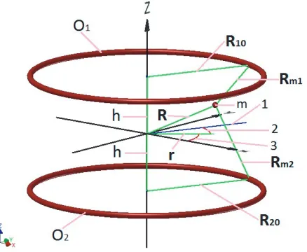
Let us consider the motion of a charged point particle in the electrostatic field of two coaxial likely charged rings located at the distance 2h (h > 0) relatively to one another. The signs of both rings’ and particle’s charges are the same. The radii of rings are equal. The linear charge densities of rings are equal. The planes within which the circles of rings are laying are parallel. The X and Y axes of coordinate system used for consideration of motion of the particle lay in a plane which is parallel to those of circles of rings and located in the middle between the planes of circles of rings. Projections of centres of circles of rings onto theX,Yplane coincide. A positive axisZoriginates from the point of projections of centres of circles of rings to the X,Y plane and is directed toward the O1 ring. The determination order of coordinates is (X, Y, Z). Coordinates of the centre of O1 ring are (0,0, h). Coordinates of the centre ofO2 ring are (0,0,−h). Coordinates of the particle location are (x, y, z).
In order to determine equations of motion of the charged particle under the action of Coulomb forces of charges of rings, we shall use the following variables and constants represented in the CGS system of units:
q is an electric charge of the particle;
R=x+y+z is a radius vector of particle’s location in the X,Y,Zcoordinate system; r=x+y;
ϕ is an angle between the X and rvectors (the direction of angle reference is counter-clockwise from theX axis toward theY axis;
˙
ϕ=dϕ/dtis a projection of vector of angular velocity of rotation of thervector onto theZaxis; R10 is a vector which radiates from the centre ofO1 ring toward the point of this circle;
R20 is a vector which radiates from the centre ofO2 ring toward the point of this circle;
Rm1 is a vector which originates from the point of O1 circle where the R10 comes in to the point of particle’s location;
Rm2 is a vector which originates from the point of O2 circle where the R20 comes in to the point of particle’s location;
φis an angle between the rvector and projection of theR10 vector onto the X,Y plane, equal to that between thervector and projection of theR20vector onto theX,Y plane (projections ofR10 andR20 vectors onto the X,Y plane coincide).
The geometry defined with the symbols introduced above is shown at Figure 1.
Figure 1. m is a particle; 1 is projections ofR10 and R20 vectors on theX,Y plane; 2 is a φangle; 3 is aϕangle.
Using the definition of potential [5], let us find the potential energy of particle in the system of two rings:
U(r, z) = qQ 2π
2π
0
1 Rm1
+ 1
Rm2
dφ, (3)
where:
Rm1 = R−hzˆ−R10, (4)
Rm2 = R+hzˆ−R20, (5)
Rm1 =
R20+ (h−z)2+r2−2rR0cos (φ)
1/2
, (6)
Rm2 =
R20+ (h+z) 2
+r2−2rR0cos (φ)
1/2
. (7)
In Eqs. (4) and (5), ˆz defines a unit vector of positive Z axis, and h is a halved distance between the centres of rings, whereas in Eqs. (6) and (7), R0 is the radius of rings. In Eq. (3), the integration is performed with respect to φ variable, with constants R0, R, h and variables Rm1 and Rm2, which depend on φ. We introduced two dimensionless variables:
˘ r= r
R0, ˘ z= z
R0,
we also introduced a dimensionless constant:
˘ h= h
R0.
(9)
Then we marked all dimensionless variable and constant functions with a semicircle sign above the symbol defining the function. First, the introduction of dimensionless functions allowed to write more compact equations of motion of particle, second, it allowed to calculate the parameters of particle motion trajectory in dimensionless values regardless of particular physical values that determine the motion of particle. In order to shorten the notation of function of electrostatic potential of the system of two rings, we introduced two dimensionless functions of two above-introduced dimensionless variables and one dimensionless constant:
˘
f1 = 1 +
˘ h−z˘
2 + ˘r2
1/2
, f˘2= 1 +
˘ h+ ˘z
2 + ˘r2
1/2
. (10)
For the purpose of determination of integral in Equation (3) using Eqs. (8)–(10), we introduced two auxiliary functions:
˘ k1=
˘ r ˘ f12
, ˘k2 = ˘ r ˘ f22
. (11)
Applying Eqs. (6)–(11):
Rm1 = R0
1 + h R0 −
z R0
2 + r
2
R20
−2 r R0
cos (φ)
1/2
=R0f˘1
1−2˘k1cos (φ)
1/2 ,
Rm2 = R0
1 + h R0 + z R0 2 + r 2 R2 0
−2 r R0
cos (φ)
1/2
=R0f˘2
1−2˘k2cos (φ)
1/2
,
we transformed Eq. (3):
U(r, z) = qQ 2πR0
2π 0 ⎛ ⎜ ⎝ 1 ˘ f1
1−2˘k1cos (φ)
1/2 +
1
˘ f2
1−2˘k2cos (φ)
1/2
⎞ ⎟
⎠dφ. (12)
As follows from Eqs. (8)–(11), if:
˘
z= ˘h, ˘r= 1, (13)
then:
2˘k1= 1, (14)
whereas if:
˘
z=−˘h, r˘= 1, (15)
then:
2˘k2= 1. (16)
For the rest values of ˘z and ˘r, the following condition is fulfilled:
2˘r <1 +
˘ h±˘z
2
+ ˘r2, r˘= 1, |z˘| = ˘h.
Consequently:
0≤2˘k1 <1, 0≤2˘k2 <1, r˘= 1, |z˘| = ˘h.
Thus, while excluding conditions of coincidence of particle location with a point on the circle of one of the rings in Eqs. (13)–(16), we could use the binomial expansion in Eq. (1) for Eq. (12):
U(r, z) = qQ 2πR0
∞
n=0 (2n)! 2n(n!)2
˘ k1n
˘ f1
+ ˘ k2n
˘ f2
2π
0
Using the values of definite integrals in Eq. (2), we integrate Eq. (17):
U(r, z) = qQ R0
∞
n=0
(4n)! 22n((2n)!)2
˘ k12n
˘ f1
+ ˘ k22n
˘ f2
(2n)! 22n(n!)2 =
qQ R0
∞
n=0
(4n)! 24n(2n)! (n!)2
˘ k12n
˘ f1
+ ˘ k22n
˘ f2
. (18)
Substituting the values of auxiliary functions in Eq. (11) to Eq. (18), we obtained the potential energy of the particle in the system of two rings:
U(r, z) = qQ R0
∞
n=0
(4n)!˘r2n 24n(2n)! (n!)2
1 ˘ f14n+1
+ 1
˘ f24n+1
. (19)
Using the generalised coordinates r, z, ϕ and generalised velocities ˙r, ˙z, ˙ϕ correspondingly, let us determine a Lagrangian of the system:
L= m
2
˙
r2+ ˙z2+r2ϕ˙2−U(r, z). (20)
Proceeding from Eq. (20), we obtain an integral of projection of moment of momentum of the particle onto the Z axis:
mr2ϕ˙ =J, J =Const, (21)
we also obtain an integral of energy:
E = m
2
˙
r2+ ˙z2+r2ϕ˙2+U(r, z), E=Const. (22)
Proceeding from Eqs. (22) and (21), we determine a function of squared projection of velocity of the particle onto thervector:
˙
r2= 2E m −z˙
2− J2
m2r2 − 2
mU(r, z). (23)
Using the Lagrangian Eq. (20) and the integral in Eq. (21), we obtain a function of projection of acceleration of the particle onto the rvector:
¨
r= J
2
m2r3 − 1 m
∂U(r, z)
∂r , (24)
From tEq. (20) we also have a function of projection of acceleration of the particle onto theZaxis:
¨ z=−1
m
∂U(r, z)
∂z . (25)
3. ZONES OF PARTICLE LOCALISATION AND CONFINEMENT IN THE TRAP
Using Eqs. (19), (24) and (25), we introduced and defined three dimensionless functions:
˘
U(˘r,z˘) = R0
qQU(r, z) = ∞
n=0
(4n)!˘r2n
24n(2n)! (n!)2
1 ˘ f14n+1
+ 1
˘ f24n+1
,
˘
Fr = mR 2 0
qQ r¨− J2 m2r3
, F˘z = mR 2 0z¨
qQ .
(26)
Then, proceeding from Eqs. (19) and (24), we obtained the following:
˘
Fr =−R 2 0
∂U(r, z)
∂r =−
∂U˘(˘r,z˘)
∂r˘ . (27)
And proceeding from Eqs. (19) and (25), we had the following:
˘
Fz =−R 2 0
∂U(r, z)
∂z =−
∂U˘(˘r,z˘)
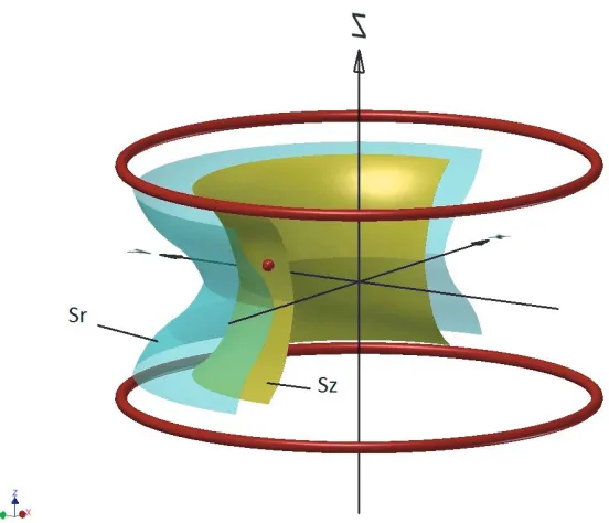
Figure 2. Zones of localisation and ejection of the charged particle during its interaction with two charged rings at ˘h= 0.5.
Graphing the dependence of dimensionless functions ˘Fr in Eq. (27) and ˘Fz in Eq. (28) on the ˘r values at various values of ˘z and ˘h allows for the following conclusions:
Under the ˘h < 2−1/2 condition, there is a particular set of trajectories of motion of the particles, while moving along which the particle will be localised in the internal space between the rings. Particles which trajectories are not in this set will be ejected from the system of rings.
Figure 2 demonstrates two surfaces (Sr and Sz) that split the space between two rings onto three zones. For visual clarity, the surfaces halved by theX,Zplane are shown. The particle located in the area between these surfaces undergoes the action of two forces which are determined by dimensionless functions in Eqs. (27) and (28), provided that ˘h = 1/2: being paralleled to the Z axis, the force is directed toward the X,Y plane; being paralleled to the r vector, it is directed toward theZ axis. At the Sr surface the magnitude of force acting on the particle in parallel to the r vector equals to zero. At the Sz surface the magnitude of force acting on the particle in parallel to the Zaxis equals to zero. In the area contacting to the Sr surface, excluding the space between the Sr and Sz surfaces, the force acting on the particle in parallel to thervector is directed away from theZaxis. In the area contacting to the Sz surface, excluding the space between the Sr and Sz surfaces, the force acting on the particle in parallel to theZaxis is directed away from the X,Y plane. Therefore, in the area between the Sr and Sz surfaces there will exist a particular set of trajectories, while moving along which the particle will be localised. If the particle enters the area beyond the Sz surface, it is repelled from the zone between the rings with the force that is directed parallel to the Z axis and away from the X,Y plane. If the particle enters the area beyond the Sr surface, it is repelled from the zone between the rings with the force that is directed parallel to the rvector and away from the Zaxis.
Only those particles can be localised in the internal space between the rings that are under some particular initial conditions of motion relatively to the charged rings. Particles whose initial conditions of motion do not match the localisation conditions will be ejected from the system of rings.
4. PARTICLE LOCALISATION CONDITIONS
functions of r variable from Eqs. (23) and (24) in order to describe the motion of particle in the X,Y plane:
˙
r2= 2E
m −
J2 m2r2 −
2
mU(r). (29)
¨
r = J
2
m2r3 − 1 m
∂U(r)
∂r . (30)
In this case, while substituting the ˘f1 and ˘f2 with their definitions (10):
U(r, z) = qQ R0
∞
n=0
(4n)!˘r2n 24n(2n)! (n!)2
⎛ ⎜ ⎜ ⎜ ⎝ 1 1 + ˘ h−z˘
2 + ˘r2
2n+1/2 +
1
1 +
˘ h+ ˘z
2 + ˘r2
2n+1/2
⎞ ⎟ ⎟ ⎟ ⎠, (31)
we could consider the potential energy of particle in Eq. (19) as a function of r variable:
U(r) = qQ R0
∞
n=0
2 (4n)! 24n(2n)! (n!)2
˘ r2n
1 + ˘h2+ ˘r22n+1/2
. (32)
The conditions of localisation of the particle on a circular trajectory whose radius is rs within the X,Y plane to be determined from those of equality of both projection of the velocity in Eq. (29) and acceleration in Eq. (30) onto the rvector to zero:
E− J
2
2mr2 s −U
(rs) = 0, J 2
mr3 s −
∂U(rs)
∂rs = 0, 0< rs< R0. (33) Proceeding from Eq. (33), we obtain the value of integral of moment of momentum and that of integral of energy of the particle localised on the circular trajectory whiose radius isrs within the X,Y plane:
Js= mrs3∂U(rs) ∂rs
1/2
, Es = rs 2
∂U(rs)
∂rs +U(rs), 0< rs< R0, (34) expressed via a radius rs of the circular trajectory. Based on Eqs. (21) and (29), using Eq. (34), we obtain an initial angular rotation velocity ˙ϕ0 of the r vector and a projection of initial velocity ˙r0 of the particle onto thervector if the particle starts its motion from the distance r0 from the Zaxis and becomes localised on the circular trajectory whose radius is rs at initial values z0= 0 and ˙z0= 0:
˙
ϕ0= Js
mr02
, r˙0=− 2Es
m −
Js2 m2r2
0
− 2
mU(r0) 1/2
, r0 > rs. (35)
The kinetic energy of particle localised on the circular trajectory whose radius isrs will be determined as follows:
mv2
2 =
Js2 2mr2
s =
rs 2
∂U(rs)
∂rs . (36)
Forrs and r0 values with a particular value of 0<˘h <2−1/2 the following condition shall fulfil:
lim
z→0z <¨ 0, rs ≤r≤r0, (37)
where the ¨z function of r and zwas determined in Eq. (25). While the condition in Eq. (37) fulfils the acceleration alongZof localising particle which is always negative, i.e., it is always directed toward the X,Y plane in the case of small variations of particle location alongZ.
5. PARTICLE LOCALISATION TRAJECTORIES
We defined a dimensionless function: ˘
A= mR0 2qQ
dr dt
2
, (38)
of dr/dtvariable and a dimensionless function:
˘ U(˘r) =
∞
n=0
2 (4n)!
24n(2n)! (n!)2
˘ r2n
1 + ˘h2+ ˘r22n+1/2
, (39)
of ˘r variable. Then we introduced two dimensionless constants:
˘
B = ER0
qQ , C˘ = J2 2mqQR0.
(40)
We rewrote Eq. (29) as follows:
dr dt
2 = 2E
m −
J2 m2r2 −
2
mU(r). (41)
Using Eqs. (38)–(40) and (41), we defined the ˘A function which was previously defined as Eq. (38) through the ˘r variable:
˘
A(˘r) = ˘B− C˘ ˘
r2 −U˘(˘r). (42)
We find continuously the first, second and third derivatives of ˘A(˘r) with respect to ˘r and determine three functions of ˘C, ˘r and ˘h:
dA˘(˘r) d˘r =
2 ˘C ˘ r3 −
dU˘(˘r)
d˘r . (43)
d2A˘(˘r) dr˘2 = −
6 ˘C ˘ r4 −
d2U˘(˘r)
d˘r2 . (44)
d3A˘(˘r) dr˘3 =
24 ˘C ˘ r5 −
d3U˘(˘r)
dr˘3 . (45)
We equate to zero the values of both the ˘A(˘r) function and its first and second derivatives of Eqs. (42) to (44), and then we form a system of three algebraic equations relatively to three unknowns ˘B, ˘C, ˘
rs =rs/R0 that depend on the value of ˘h:
1. B˘ = C˘ ˘ r2
s + ˘U(˘rs), 2. ˘ C = ˘r
3 s 2
dU˘(˘rs) d˘rs , 3.
3 ˘ rs
dU˘(˘rs) d˘rs =−
d2U˘(˘rs) dr˘2
s . (46)
We equate to zero the value of the third derivative of ˘A(˘r) function and obtain the following inequality:
12 ˘ r2
s
dU˘(˘rs)
d˘rs =
d3U˘(˘rs)
dr˘3
s , (47)
that we shall use for determination of range of values ˘h for which both the system of Equations (46) and the inequality of Eq. (47) are valid. The system of Equations (46) and the inequality of Eq. (47) determine conditions under which the ˘A(˘r) function of Eq. (42) has an inflection point at which the value of function equals zero. As also follows from these conditions, the function in Eq. (43) has an extremum in the point of inflection of function in Eq. (42), at this extremum point the function in Eq. (43) equals zero as well. The function in Eq. (42) is a dimensionless function of the squared radial velocity of particle (the radial velocity is a projection of velocity onto the rvector):
˘
A(˘r) = mR0 2qQ
dr dt
2
The function in Eq. (43) is a dimensionless function of radial acceleration of particle (the radial acceleration is a projection of acceleration onto the rvector):
dA˘(˘r) dr˘ =
mR20
qQ d2r dt2.
Therefore, in the point of inflection of the ˘A(˘r) function in Eq. (42) the radial velocity and radial acceleration of particle shall equal zero. The particle being under the initial conditions of motion determined from Eqs. (46) and (47), with negative value of initial radial velocity shall overcome the repulsion of rings, and its trajectory will gradually transform to circle with particular constant values of ˘rs and ˙ϕ.
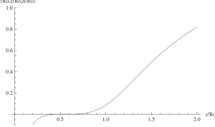
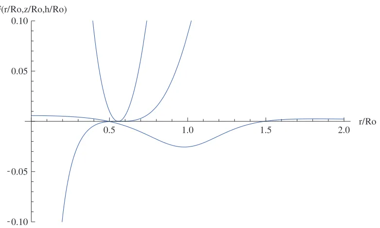
The dynamics of particle which moves from the dimensionless distance to the origin of coordinate system of ˘r0 = 2 (˘r0 = r0/R0) toward the rings and has a trajectory that transforms to circle as determined by conditions in Eqs. (46) to (47) with ˘h = 1/2 is demonstrated in Figures 3 to 5. The figures show the graphs of three functions:
– the graph in Figure 3 determines the values of function of squared dimensionless radial velocity of particle depending on the distance to the origin of coordinate system (the ˘A(˘r) function in Eq. (42) for which the values of constants ˘B and ˘C were obtained from the system of Equations (46) with ˘
h= 1/2);
– the graph in Figure 4 determines the values of function of dimensionless radial acceleration of particle depending on the distance to the origin of coordinate system (the dA˘(˘r)/d˘r function in Eq. (43));
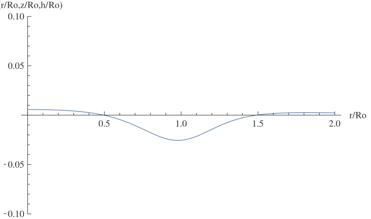
– the graph in Figure 5 determines the values of function of dimensionless force acting on the particle in parallel to the Zaxis (if the values are negative, then the forces strain the particle to theX,Y plane) depending on the distance to the origin of coordinate system with ˘z= 0.01 and with ˘h= 1/2 (the ˘Fz function in Eq. (28)).
0.5 1.0 1.5 2.0 r/Ro
0.2 0.4 0.6 0.8 1.0
F(r/Ro,z/Ro,h/Ro)
Figure 3. The graph of function of squared dimensionless radial velocity of particle.
0.5 1.0 1.5 2.0 r/Ro 0.2
0.4 0.6 0.8 1.0
F(r/Ro,z/Ro,h/Ro)
Figure 4. The graph of function of dimensionless radial acceleration of particle.
0.5 1.0 1.5 2.0 r/Ro
- 0.10 - 0.05 0.05 0.10
F(r/Ro,z/Ro,h/Ro)
Figure 5. The graph of function of dimensionless force acting on the particle in parallel to theZaxis.
Being a dependency of ˘r on ϕ, the particle’s motion in the X,Y plane could be routed using the equation obtained from Eq. (42), substituting dt in the ˘A function, which was defined as in Eq. (38), withdϕ obtained from Eq. (21):
dr˘ dϕ
2 = r˘
4
˘ C
˘ B−
˘ C ˘
r2 −U˘(˘r)
, (48)
using the Taylor formula:
˘
r(ϕn+1) = ˘r(ϕn) + K
k=1 1 k!
∂k˘r(ϕn)
∂ϕkn (ϕn+1−ϕn)
0.5 1.0 1.5 2.0 r/Ro
- 0.10 - 0.05 0.05 0.10
F(r/Ro,z/Ro,h/Ro)
Figure 6. The dynamics of localisation of charged particle during its interaction with two charged rings.
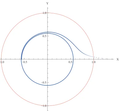
The trajectory of localising particle whose initial conditions of motion are determined from the system of Equations (46) with ˘h= 0.5 and with initial ˘r0= 1.4 is demonstrated in Figure 7. This trajectory was traced using Eqs. (48) and (49) across the points with K = 2 with angular step ϕn+1−ϕn = 3π/1000 while ϕ varied from 0 to 3π. The unit radius circle at Figure 7 is a projection of circles of charged rings onto the X,Y plane whose dimensionless radii are determined as ˘R0 =R0/R0. The overall sum of moduli of corrections to the values of ˘r calculated with K = 2 for all points used for tracing the trajectory do not increase the value of 0.010254 if the ˘r values were calculated withK = 10.
The analytical research and numerical simulations demonstrate that circular trajectories of localisation of particles within the X,Y plane are determined by dimensionless radii of trajectories within the range of values ˘rmin ≤r˘s <r˘max where ˘rmin is the inflection point of the ˘A(˘r) function in Eq. (42) for which the values of constants ˘Band ˘Cto be calculated based on the system of Equations (46) under the condition in Eq.(47), and the value ˘rmaxis determined from the equation ˘C = 0 with particular values of ˘h.
The initial conditions of motion of particle, which is localised on the circular trajectory with dimensionless radius ˘rswithin theX,Yplane, being expressed via the ˘Band ˘Cconstants are determined according to the following algorithm:
0<˘h <2−1/2, r˘min≤˘rs<r˘max, U˘(˘rs) = ∞
n=0
2 (4n)! 24n(2n)! (n!)2
˘ rs2n
1 + ˘h2+ ˘r2 s
2n+1/2. (50)
The value of ˘rmin is a real positive root of algebraic equation obtained from the Equation 3 of Eq. (46):
3 x
∂U˘(x)
∂x +
∂2U˘(x)
∂x2 = 0, 0< x <1, (51)
with regard to an unknown x. The value of ˘rmax is a real positive root of algebraic equation obtained from Equation 2 of Eq. (46):
∂U˘(x)
-1.0 -0.5 0.5 1.0 X
- 1.0 - 0.5 0.5 1.0 Y
Figure 7. The trajectory of localising particle with ˘h = 0.5, ˘B ≈ 1.84007, ˘C ≈ 0.00565, and with ˘
r0 = 1.4.
also with regard to an unknownx. The values of ˘B and ˘C constants are determined from Equations 1 and 2 of Eq. (46) as:
˘ B = C˘
˘ r2
s + ˘U(˘rs), ˘ C = r˘
3 s 2
∂U˘(˘rs)
∂˘rs . (53)
Then from Eqs. (38) and (42), we shall obtain the value of initial radial velocity and from Eq. (40) that of initial angular velocity of particle:
˙ r0 =−
2qQ mR0
˘ B− C˘
˘ r02
−U˘(˘r0)
1/2
, ϕ˙0=
2qQC˘ mR30r˘40
1/2
, r˘0= r0
R0.
(54)
The values of ˘r0 are determined by the condition in Eq. (37).
6. CONCLUSION
on which the particle was localised (for example, the trajectory shown at Figure 7). However, if the particle spends its energy for radiation, then it will pass to more sustainable trajectory, and for the removal of particle from it the latter shall be energised more than it required for the removal of it from the initial circular trajectory for the value of energy lost by the particle due to radiation. If theZaxis of the trap is vertical, then the gravitational acceleration of particle along theZaxis can be compensated with that from an external electrostatic field which will help to confine the particle within the X,Y plane. External electrostatic fields can be used for creation of constant negative acceleration of the particle along theZaxis, excluding the need in the conditions in Eq. (37).
If we have a source that periodically emits particles with the same charges, same masses, same magnitudes of velocity and along the same direction, we can adjust parameters of electrostatic trap so that the particles of source are localised on the same circular trajectory and move along it with the same magnitudes of velocity. The distances between the neighbour particles and magnitudes of their relative velocities will depend on the number of particles localised on this trajectory. Changing the distance between the rings or charges of rings, one can form beams of likely charged particles which relative velocities inside the beam are small. The beams can be ejected both within theX,Y plane and along the Zaxis.
Therefore, the results of analytical and numerical research of trajectories of motion of charged particles during their interaction with two likely charged rings demonstrate the following theoretical opportunities:
– localisation of likely charged particles under particular initial conditions of motion relatively to the charged rings in the space between them if the sign of particles’ charges is the same as of those of the rings;
– the long-continued confinement of likely charged particles in the localised state;
– formation of beams of likely charged particles with the small emittance, with given kinetic energy, and with given direction of motion relatively to the system of charged rings.
REFERENCES
1. Eseev, M. K. and I. N. Meshkov, “Traps for storing charged particles and antiparticles in high-precision experiments,”Phys.-Usp., Vol. 59, 304–317, 2016.
2. Major, F. G., V. N. Gheorghe, and G. Werth, Charged Particle Traps, Physics and Techniques of Charged Particle Field Confinement, Springer, Berlin, 2005.
3. Werth, G., V. N. Gheorghe, and F. G. Major, Charged Particle Traps II: Applications, Springer, Berlin, 2009.
4. Gluck, F., “Axisymmetric electric field calculation with zonal harmonic expansion,” Progress In Electromagnetics Research B, Vol. 32, 319–350, 2011.