Electronic Thesis and Dissertation Repository
6-20-2016 12:00 AM
The Development And Application Of A Statistical Shape Model Of
The Development And Application Of A Statistical Shape Model Of
The Human Craniofacial Skeleton
The Human Craniofacial Skeleton
Mark A C Neuert
The University of Western Ontario
Supervisor
Dr. Thomas R. Jenkyn
The University of Western Ontario
Graduate Program in Mechanical and Materials Engineering
A thesis submitted in partial fulfillment of the requirements for the degree in Doctor of Philosophy
© Mark A C Neuert 2016
Follow this and additional works at: https://ir.lib.uwo.ca/etd
Recommended Citation Recommended Citation
Neuert, Mark A C, "The Development And Application Of A Statistical Shape Model Of The Human Craniofacial Skeleton" (2016). Electronic Thesis and Dissertation Repository. 3905.
https://ir.lib.uwo.ca/etd/3905
This Dissertation/Thesis is brought to you for free and open access by Scholarship@Western. It has been accepted for inclusion in Electronic Thesis and Dissertation Repository by an authorized administrator of
ii
Biomechanical investigations involving the characterization of biomaterials or improvement of implant design often employ finite element (FE) analysis. However, the contemporary method of developing a FE mesh from computed tomography scans involves much manual intervention and can be a tedious process. Researchers will often focus their efforts on creating a single highly validated FE model at the expense of incorporating variability of anatomical geometry and material properties, thus limiting the applicability of their findings. The goal of this thesis was to address this issue through the use of a statistical shape model (SSM).
A SSM is a probabilistic description of the variation in the shape of a given class of object. (Additional scalar data, such as an elastic constant, can also be incorporated into the model.) By discretizing a sample (i.e. training set) of unique objects of the same class using a set of corresponding nodes, the main modes of shape variation within that shape class are discovered via principal component analysis. By combining the principal components using different linear combinations, new shape instances are created, each with its own unique geometry while retaining the characteristics of its shape class.
iii
iv
Chapter 1: Mark Neuert – sole author
Chapter 2: Mark Neuert – study design, data collection, data analysis, sole author; Claudia Blandford – study design, data collection, data analysis; Tom Jenkyn – study design, reviewed manuscript
Chapter 3: Mark Neuert – study design, data collection, data analysis, sole author; Claudia Blandford – study design, data collection, data analysis; Tom Jenkyn – study design, reviewed manuscript
Chapter 4: Mark Neuert – study design, data collection, data analysis, sole author; Meg Clynick – data collection, data analysis; Erica yang – data collection, data analysis; Ryan Willing – provided software used to calculate CFS symmetry scores; Tom Jenkyn – study design, reviewed manuscript
Chapter 5: Mark Neuert – study design, data collection, data analysis, sole author; Claudia Blandford – study design, data collection, data analysis; Timothy Burkhart – reviewed manuscript; Tom Jenkyn – study design, reviewed manuscript
v
They say that no man is an island unto himself. I’ve spent many sleepless nights wrestling with this thesis, and I’m grateful for everyone who has been in my corner.
I’d like to thank all the mentors I’ve encountered throughout my academic career. My first encounter with research was as an undergraduate at the University of Alberta, and I’d like to thank Dr. Jason Carey for showing me that research can be a fun and meaningful endeavor. I’d like to thank my Master’s supervisor, Dr. Cynthia Dunning, for inspiring within me the confidence to tackle unknown questions with confidence and fearlessness. Finally, I’d like to thank my current supervisor Dr. Tom Jenkyn, for all the support he’s provided to me throughout my PhD, and for being there when I really needed him.
I’d like to thank all my colleagues. Ryan Willing, the technical support and feedback you provided was much appreciated, as were your “Scrubs” quotes. Claudia Blandford, you were my teammate, partner in crime. You were part of the reason I came on to this project, and your impact on me has been immeasurable. Tim Burkhart, your feedback and stats help has been so appreciated, and I’m glad you remained in the BTL so I didn’t have an empty lab space to go to. Finally, Anne McDonald, thanks for challenging me so much. You’ll make a great doctor!
vi
I dedicate this thesis to my father, John, my mother, Sylvia, and my love, Tara.
“God only knows what I’d be without you.”
vii
Table of Contents
Abstract ... ii
Co-Authorship Statement (where applicable) ... iv
Acknowledgments... v
Dedication ... vi
Table of Contents ... vii
List of Tables ... xii
List of Figures ... xiv
List of Abbreviations ... xix
1 A Proposal to use Statistical Shape Modeling to Implement a Combined Monte Carlo and Finite Element Analysis of the Human Craniofacial Skeleton ... 1
1.1 Motivation and Objectives ... 1
1.2 Background ... 2
1.2.1 The Skull ... 2
1.2.2 Finite Element Modeling (FEA) ... 5
1.2.3 Probabilistic Methods and FEA in Biomechanics ... 7
1.2.4 Statistical Shape Modeling (SSM) ... 10
1.3 Outline of Research Performed ... 17
viii
1.3.3 SSM of the human CFS ... 19
1.3.4 Monte Carlo Analysis of Zygoma Fracture ... 20
1.4 Significance... 21
1.5 References ... 22
2 Validation of a Finite Element Model of the Human Craniofacial Skeleton Through Modal Analysis ... 26
2.1 Introduction ... 26
2.2 Methods... 28
2.2.1 Experimental Resonant Frequency Acquisition... 28
2.2.2 Model Creation ... 29
2.2.3 Mesh Evaluation ... 29
2.2.4 Materials Assignment ... 30
2.2.5 Boundary Conditions ... 31
2.2.6 Data Analysis ... 31
2.3 Results ... 32
2.3.1 Rigid Body Motion ... 32
2.3.2 Mesh Evaluation ... 32
2.3.3 Resonant Frequencies ... 35
ix
2.5 Conclusion ... 44
2.6 References ... 45
3 Development of a Mesh Morphing Algorithm Applied to the Craniofacial Skeleton . 48 3.1 Introduction ... 48
3.2 Methods... 51
3.2.1 Mesh Morphing Algorithm ... 51
3.2.2 Morphed Mesh Quality and Performance ... 58
3.3 Results ... 60
3.3.1 Mesh Morphing ... 60
3.3.2 Model Validation ... 62
3.4 Discussion ... 65
3.5 Conclusion ... 69
3.6 References ... 70
4 Validation of a Statistical Shape Model of the Human Craniofacial Skeleton ... 73
4.1 Introduction ... 73
4.2 Methods... 75
4.2.1 Statistical Shape Model... 75
4.2.2 Validation of SSM Generated Geometry ... 80
x
4.3.2 Validation of SSM Generated Geometry ... 88
4.4 Discussion ... 94
4.5 Conclusion ... 98
4.6 References ... 99
5 Implementation of a Statistical Shape Model of the Craniofacial Skeleton in a Monte Carlo Analysis of Zygomatic Fracture ... 102
5.1 Introduction ... 102
5.2 Methods... 105
5.2.1 FE Model creation... 105
5.2.2 Fracture Categorization ... 107
5.2.3 Correlation Between Model Features and Incidence of Fracture ... 109
5.3 Results ... 111
5.3.1 Fracture Categorization and Historical Comparison ... 111
5.3.2 Correlation Between Model Features and Incidence of Fracture ... 113
5.4 Discussion ... 115
5.5 Conclusion ... 119
5.6 References ... 121
6 Conclusion ... 124
xi
6.3 Significance... 128
6.4 Future Directions ... 129
6.5 References ... 132
Appendix A – Reprinting Permissions ... 133
Bryan et al. ... 133
Cootes et al. ... 134
Li et al. ... 135
Willing et al. ... 136
Yoganandan et al. ... 137
Zingg et al. ... 138
Appendix B – Detailed Specimen Information ... 139
Appendix C – Mesh Morphing and Natural Frequency Results for Non-Experimental Craniofacial Specimens ... 140
Appendix D – Pseudocode for the Morphing Algorithm... 143
xii
Table 2-1 - Percent change in numerically derived resonant frequency values across different mesh densities for each specimen. ... 33
Table 2-2 – Difference between experimental and calculated resonant frequency values for each specimen in terms of root mean square error, average percent error, and absolute % error. ... 35
Table 2-3 – Intra-class correlations between experimental and calculated resonant frequencies. ... 35
Table 2-4 – Average deviation and standard deviation values of frequency pairs corresponding to Bland-Altman plots. ... 39
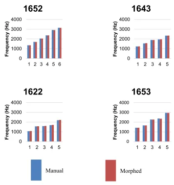
Table 3-1 – Difference between resonant frequency values calculated using manually created and morphed meshes in terms of root mean square error, average percent error, and absolute % error. ... 63
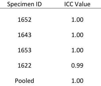
Table 3-2 – Intra-class correlations calculated for resonant frequency values as calculated using manually created and morphed meshes ... 63
Table 3-3 – Average deviation and standard deviation values of frequency pairs corresponding to Bland-Altman plots. ... 65
Table 4-1 – List of craniometric measures used in the geometric validation of SSM produced skull sample... 84
Table 4-2– Howells (sub-populations) and SSM correlation matrices. All off-diagonal correlations were significant at p < 0.01. ... 90
xiii
Table 4-5 – ICC values comparing automated and manual CFS metric measurements. .. 92
Table 5-1 – Summary of results from multivariate multiple linear regression analysis. Significant effects are bolded. The Model Significance row lists each independent variable’s p-value for the entire linear model. The Between-Subjects Effects row lists each independent variable’s p-value for a corresponding dependent variable, with beta values underneath in brackets. ... 114
xiv
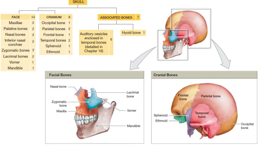
Figure 1-1 – The bones of the Cranium and Skull. Figure from Human Anatomy ©2012, Benjamin Cummings, p. 141 ... 3
Figure 1-2 – Fracture classification system as described by Zingg et al23. ... 5
Figure 1-3 – Discretization of a skull from 3-D geometry into a finite element mesh. ... 6
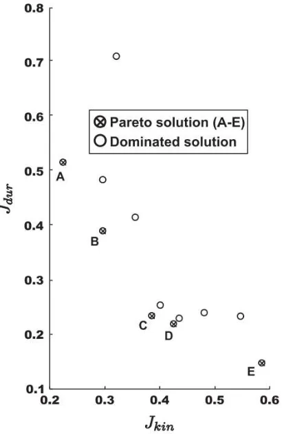
Figure 1-4 – Pareto Curve points from Willing et al.26 Traveling along the pareto solution
points, optimizing for kinematics (decreasing the value Jkin) necessitates a less optimal
solution for durability (increasing the value of Jdur) ... 8
Figure 1-5 – 5-95% knee force-displacement corridors in the anterior-posterior direction. The curves were generated in a Monte Carlo analysis where 200 unique FE models using unique ligament parameters, such as insertion points and stiffness29. ... 9
Figure 1-6 – Studies employing FE analysis of skull biomechanics. Each only used a single craniofacial geometry, focusing on parametric analyses of other parameters, such as suture formation or material properties. Figure adapted from Li et al41. ... 10
Figure 1-7 – Shape instances within an allowable shape space, along with the average shape . The shape space in this figure is represented by a 3-D ellipsoid volume for illustrative purposes, however, in reality, shape domains are commonly of many more dimensions. ... 12
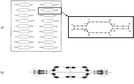
Figure 1-8 – a) A training set of electrical resistors, taken from Cootes et al. 199542, with
a set of 32 landmarks used to define each resistor in the training set. b) The average shape of the resistors showing the spread of selected individual landmarks. ... 12
xv
Figure 1-10 – The impact of varying the weighting of the largest and most influential eigenmode on resistor shape from the example in Cootes 199542. Note how each resistor is
still of the same class (i.e. is still resistor-shaped), but has a unique geometry. ... 15
Figure 1-11 – The influence on shape and material distribution due to varying the weighting of the first and most influential eigenmode between − ≤ ≤ in a statistical shape model of the femur10. It is apparent that this eigenmode mostly scales the femur axially,
with some effect on cortical thickness. ... 16
Figure 2-1 - Resonant frequency values for specimen 1641 using mesh densities with 1) no restriction on maximum edge length 2) maximum edge length restricted to 2 mm 3) maximum edge length restricted to 1 mm... 33
Figure 2-2 - Mesh element distributions for a) radius ratio ( ), b) mean ratio ( ), and c) element condition ( ) number. ... 34
Figure 2-3 – Comparison of numerically and experimentally derived resonant frequency values for each CFS specimen. ... 36
Figure 2-4 - Bland-Altman plot comparing experimental (gold standard) and calculated values for all resonant frequencies of all specimens. The average error is -206 Hz with a standard deviation of 296 Hz. The blue line is the average deviation and the red lines represent a 95% confidence interval (±1.96σ). ... 37
Figure 2-5 – Bland-Altman plots comparing experimental (gold standard) and calculated values for all resonant frequencies for individual specimens. The blue line is the average deviation and the red lines represent a 95% confidence interval (±1.96σ). ... 38
xvi
the are determined going from to , will be determined for to . ... 53
Figure 3-2 – 2-D illustration of mesh untangling process. a) Tangled elements (red) are identified, and their connected nodes (light blue) grouped into a sub-set. b) Proceeding serially through the node sub-set, a sub-mesh is created (green and red) by selecting all elements connected to the current node (dark blue). c) The untangling algorithm operates on the sub-mesh by minimizing the sum of the inverse element scores of the submesh, simultaneously untangling elements and improving element quality. d) The algorithm moves to the next node in the sub-set (dark blue). If the submesh produced by this node is already untangled, the algorithm proceeds to the next node. ... 57
Figure 3-3 – Averaged cumulative distribution curves of ρ, κ, and η for morphed (red) and manually created (black) meshes. For all measures, maximum corridor width was 0.02 for manual meshes and 0.05 for morphed meshes... 61
Figure 3-4 – Comparison of resonant frequency values as calculated using manually created and morphed meshes. ... 62
Figure 3-5 – Pooled Bland-Altman plot comparing the resonant frequencies using manually created (gold standard) and morphed meshes. The blue line represents the average deviation with red lines representing a 95% confidence interval. ... 64
Figure 3-6 – Bland-Altman plots of FE calculated resonant frequencies using manually created (gold standard) and morphed meshes. The blue line represents the average deviation with red lines representing a 95% confidence interval. ... 64
xvii
highlighted. ... 77
Figure 4-2 – Representation of the average skull shape from the training set. ... 82
Figure 4-3 – Eigenvalue decay representing the accumulated percentage of shape and stiffness variation inherent in the SSM training set. ... 85
Figure 4-4 – Visualizations of +/-2σ (green/red) of the first 9 (E1-E9) eigenvectors for CFS geometry ... 86
Figure 4-5 – Visualizations of +/-2σ of the first 9 (E1-E9) eigenvectors for CFS stiffness distribution ... 87
Figure 4-6 – Comparison of symmetry scores between SSM produced CFS models and a population of 32 specimens from Willing et al using a whisker plot. The red line represents the median, the lower and upper blue boundaries represent the 25th and 75th percentiles
respectively, and the whiskers extend to the most extreme values. ... 88
Figure 4-7 – Scatterplots of the relationship between cranial braedth (XCB) and a) facial breadth (ZYB), facial height (NPH), and cranial length (GOL). ... 89
Figure 4-8 – Comparison of normalized craniometric measurement distributions using a) all Howells data and b) Howells specimens of European descent. Measurement values (mm) are on the x-axis, with proportion of total population on the y-axis. ... 91
Figure 4-9 – Bland-Altman plots comparing CFS dimensions measured using manual and automated methods (mm). ... 93 Figure 5-1 –a) Loading node set and b) load direction axis used for the FE simulations. ... 106
xviii
Figure 5-4 – Inferior view of the craniofacial skeleton showing craniometric measurements
investigated for association with craniofacial fractures ... 110
Figure 5-5 - Proportion of finite element simulation resulting in at least one ROI experiencing fracture. ... 111
Figure 5-6 – Breakdown of fracture types as predicted by finite element simulations. . 112
Figure 5-7 - Representative examples of FE simulations resulting in fractures of types A1, A2, A3, and B/C... 112
Figure C-1 - Averaged cumulative distribution element quality curves of ρ, κ, and η for morphed (red) and manually created (black) meshes. For all measures, maximum corridor width was 0.02 for manual and 0.05 for morphed meshes. ... 141
Figure C-2 – Bland-Altman plot comparing the FE calculated free vibration natural frequency values using manually created (the gold standard reference) and morphed meshes. ... 142
Figure D-1 – Pseudocode for Morph ... 144
Figure D-2 – Pseudocode for calc_def_field_subset ... 145
Figure D-3 – Pseudocode for calc_disp_field ... 146
Figure D-4 – Pseudocode for diffusion_main ... 147
xix CFS – Craniofacial skeleton.
EUL/EUR – Location of the left/right euryons, the most extremely lateral points on the cranial braincase.
FE – Finite element (as in Finite Element Mesh).
G – Location of the glabella, a smooth, raised region on the frontal bone just above the nasion and between the eyebrows.
GOL – Cranial length (Gonion-Opisthocranion distance).
Hz – Hertz, unit of measure for frequency.
MC – Monte Carlo (as in Monte Carlo Analysis).
N – Location of the nasion, the point in the midline of the face where the nasal and frontal bones intersect.
NPH – Facial height (nasion-prosthion distance).
O – Location of opisthocranion, the most extremely posterior point on the cranium in the
SSM – Statistical shape model.
P – Location of prosthion, the most anterior point on the maxillary alveolar process in the sagittal plane.
XCB – Cranial breadth (distance between the euryons).
ZYB – Facial breadth (distance between the zygions).
1
A Proposal to use Statistical Shape Modeling to
Implement a Combined Monte Carlo and Finite Element
Analysis of the Human Craniofacial Skeleton
1.1 Motivation and Objectives
The human craniofacial skeleton (skull) is the primary structure protecting the brain from external trauma. There is growing evidence that facial fractures are associated with both minor and major brain damage1, and considering that in 2007, the management of skull
fractures topped $1 billion in the United States alone2, the importance of understanding the
mechanics of skull impact and fracture has never been more apparent.
Through various modes of instrumentation, researchers have attempted to measure the forces, strains, and accelerations characterizing skull fracture3–9; however, many of these
studies are necessarily destructive, making it difficult and expensive to explore different combinations of fracture conditions. Furthermore, the amount of detail that can be acquired from physical experiments is limited, as transducers such as strain gauges only collect data at discrete locations.
To address this issue, probabilistic methods have been used to incorporate geometric variability in FE analysis. Statistical shape modeling (SSM) quantifies the primary modes of shape variation in a sample (or “training set”) of a given class of object (e.g. the skull) using principal component analysis (PCA). By exploring the shape space as defined by the space’s principal components, a unique shape instance can be created. Applied to FE analysis, SSM can automate the generation of an arbitrary number of FE meshes, each with a unique size and shape. This approach has already been used in analyses of the femur10– 12, shoulder13, and knee14. The objective of and motivation behind this thesis is to use SSM
as a tool to incorporate the geometric and material variability in FE analysis of the craniofacial skeleton (CFS), and to demonstrate the utility of such a model to improve real-world biomechanical surrogates.
1.2 Background
1.2.1 The Skull
1.2.1.1 Anatomy & Structure
Figure 1-1 – The bones of the Cranium and Skull. Figure from Human Anatomy
©2012, Benjamin Cummings, p. 141
The bones of the face provide additional attachment points for facial muscles, and support features of the digestive and respiratory tracts. These include the maxillae, palatine bones, nasal bones, inferior nasal conchae, lacrimal bones, the vomer, mandible, and the zygomatic bones15.
1.2.1.2 Fracture of the Zygoma
The zygoma forms the prominent structure on the upper check, just inferior and lateral to the orbit. It forms one of the main buttress structures of the face, transmitting force from the dentition to the cranial base, and as such, it is made of dense cortical bone.
This is primarily due to its exposed position on the side of the face, making it particularly vulnerable in cases of assault or sporting incidents. The zygoma is also commonly fractured as a result of the face impacting the steering wheel due to vehicular collisions, an occurrence which persists despite the development of safety design features such as energy-absorbing wheels and airbags17.
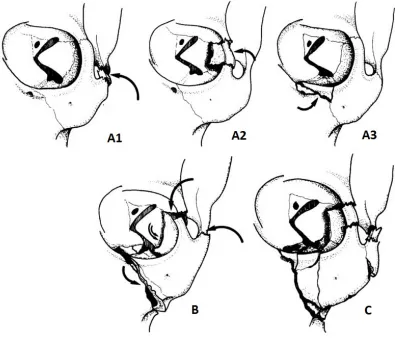
Despite several attempts to classify fractures of the zygoma18–21, no single classification
system that has been widely adopted due to the many ways in which fractures can present22.
The most favored system is that developed by Zingg et al, which accounts for the three-dimensional nature of zygomatic fracture (which often includes dislocation), and describes fracture with respect to the zygoma’s articulations with other major bones of the face23,24.
Figure 1-2 – Fracture classification system as described by Zingg et al23.
1.2.2 Finite Element Modeling (FEA)
1.2.2.1 What Is FEA?
mesh fineness. In general, a fine mesh (i.e., many small elements) is more accurate than a coarse mesh (i.e., fewer large elements), creating a trade-off between model accuracy and computation time; however, computer hardware has developed to the point where FE meshes composed of millions of elements can be solved in a matter of hours.
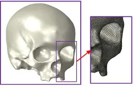
Figure 1-3 – Discretization of a skull from 3-D geometry into a finite element mesh.
1.2.2.2 FEA in Biomechanics
Once a FE model is validated, input parameters can be changed relatively easily (and cheaply) in computer software. This sort of flexibility facilitates parametric analysis, where model inputs are varied, or perturbed, to quantify their effects on corresponding outputs25.
Parametric analysis has been quite fruitful in the field of biomechanics, yielding a valuable tool in the characterization of design objectives in orthopaedic implants26, improving the
understanding of the elastic properties of bone 27, and predicting the response of bone to
different implant designs28, to name just a few applications.
1.2.3 Probabilistic Methods and FEA in Biomechanics
The existence of variability in biomechanical parameters such as anatomic geometry, material properties, and the insertion points of ligaments and tendons, is a pervasive issue in biomechanical research. It is important to acknowledge that this variability has a large effect on the outcomes of patient interventions such as orthopaedic joint replacement or reconstructive surgery. As a result, biomechanical studies that don’t account for the full spectrum of parameter values may be limited in their application.
in a Pareto Curve (Figure 1-4), which describes the limit where changing design parameters to improve one design objective necessarily reduces performance in a competing objective.
Parametric analyses of biomechanical
systems
reveal how outcomes might change with respect to inputs, which can yield very useful information. However, just as important is the determination of the likelihood of any particular outcome. An FE analysis is a deterministic model, however the inputs exist as probabilistic distributions, which need to be accounted for when considering whether or not a specific combination of variables, and thus a specific outcome, is likely to occur.Figure 1-5 – 5-95% knee force-displacement corridors in the anterior-posterior direction. The curves were generated in a Monte Carlo analysis where 200 unique FE models using unique ligament parameters, such as insertion points and
stiffness29.
The Monte Carlo (MC) method is one approach researchers have taken to incorporate parameter probability. In MC analysis, input parameters are sampled randomly from their respective probabilistic distributions, with the resulting distribution of the output variable(s) characterizing the likelihood of a given result. For example, Baldwin et al.
performed 200 FE analyses of the knee joint while randomly varying ligament stiffness, reference strain, and attachment point locations to generate 5-95 percentile corridors describing the force-displacement behavior of anterior-posterior and internal-external laxity in the knee joint (Figure 1-5)29. MC analysis has also been applied to study the
influence of material properties in cervical spine on disc annulus stress30, as well as
activation levels of lower limb muscles on knee loading31, and other examples involving
1.2.4 Statistical Shape Modeling (SSM)
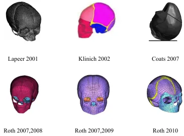
Variation of mesh-independent inputs, such as insertion points or material properties, can be incorporated into a FE model simply by specifying a configuration vector in a programming script. However, accounting for variation in anatomical shape is a much more challenging problem because making an individual FE mesh from a CT scan is a tedious procedure. While commercial software packages provide sophisticated algorithms for extracting and meshing geometry from medical images, bone shapes are highly irregular, and a quality mesh requires much manual intervention. Thus, many FE investigations of the skull use small samples (some as few as one), putting more effort into increasing the accuracy and fidelity of a single model at the expense of the ability to generalize due to under-representation of geometric variability35–40 (Figure 1-6).
Lapeer 2001 Klinich 2002 Coats 2007
Roth 2007,2008 Roth 2007,2009 Roth 2010
While much can be gained from a single, thoroughly validated model, there is great potential in creating tools that would allow FE analyses to incorporate geometric variability. Recently, researchers have turned to Statistical Shape Modeling to achieve this. Statistical Shape Modeling (SSM) is a procedure originally developed in image processing that has been used to describe shape variation inherent in a particular class of object42. By
training a single mesh topology to a set of training objects that are of the same class, a SSM can automatically produce new unique geometries within that shape class.
1.2.4.1 Implementation of SSM
In SSM, m objects of the same class (e.g.m skulls) form a training set, or representative sample, and are subsequently discretized using a set of corresponding landmarks. After first describing all instances in a common coordinate system (hence eliminating variation in position among training set instances, which is rarely of interest), each instance is recorded as a unique point, in a domain called an allowable shape space. The shape space consists of ×n dimensions, where n is the number of landmarks used to discretize a shape andd is the number of degrees of freedom required to define each landmark:
= , , , … , , … × , = 1 …
The average shape of the m training set objects is calculated as in Figure 1-7. Figure 1-8 illustrates this procedure using a simple 2-D example involving training the outline of a set of electrical resistors, as it was presented in the seminal shape modeling paper by Cootes
et al.42. Each resistor is defined using 32 corresponding landmarks (i.e., n = 32), where
= 1
Figure 1-7 – Shape instances within an allowable shape space, along with the average shape . The shape space in this figure is represented by a 3-D ellipsoid volume for illustrative purposes, however, in reality, shape domains are commonly of many more dimensions.
a)
b)
Principal component analysis (PCA) is then used to describe the variation between the training set objects within the shape space. First, the deviation of each object from is calculated:
= − (3)
from which a covariance matrix is calculated:
= 1 (4)
The eigenvectors , and corresponding eigenvalues , of are:
= (5)
Figure 1-9 – The modes of variation of points within the shape space are defined by three principal components in this simplified 3-dimentional example. Since the thickness of the space in the direction of PC3 is small (the 3-D volume is squished into a thin disk) compared to PCs 1 and 2, most of the variation of the data occurs with respect to PCs 1 and 2, and the 3-D shape space can be approximated as a 2-D circle without sacrificing much information of the total variability in the shape space.
Combining the average shape plus a linear combination of eigenvectors creates a unique shape within the shape space:
= + (6)
Figure 1-10 – The impact of varying the weighting of the largest and most influential eigenmode on resistor shape from the example in Cootes 199542. Note how each resistor is still of the same class (i.e. is still resistor-shaped), but has a unique geometry.
1.2.4.2 SSM in Biomechanics
Due to computing constraints at the time of its development, early implementations of SSM in biomechanics used only 2-dimensional landmarks (d = 2)43,44. Since computing
capabilities have progressed, 3-D, 4-D, and higher dimensional landmarks (dimensions higher than three involve assigning scalar values, such as temperature, concentration, or density to nodes in addition to coordinates) have been incorporated as well.
Using a training set of 21 femurs, Bryan et al.10 used SSM to drive a Monte Carlo analysis
Figure 1-11 – The influence on shape and material distribution due to varying the weighting of the first and most influential eigenmode between − ≤ ≤ in a statistical shape model of the femur10. It is apparent that this eigenmode mostly scales the femur axially, with some effect on cortical thickness.
Statistical shape modeling has also been applied to systems of multiple structures. Yang et al.13 applied SSM to the primate shoulder, modeling humerus and scapula alignment, while
Baldwin et al. 14 applied SSM to soft tissue structures, predicting variations in cartilage
thickness and alignment in the knee joint.
There is currently only one study41 which applies SSM to the skull. The training set for this
model contained infants of 0–3 months of age, a developmental period that displays extreme changes shape. The goal of this study was to understand how certain craniometric measurements of the skull related to one another over time during early human development.
with other landmarks. Skull thickness was also of interest, and thus thickness values were manually measured at each landmark, requiring further manual intervention. These requirements resulted in a much increased time requirement to develop the training set as compared to previously described automated studies investigating the femur10.
1.3 Outline of Research Performed
The goal of this thesis is to develop computational tools necessary to create and validate a SSM of the CFS of the adult human, to use these tools to automatically generate unique FE meshes of the CFS, and to use these meshes in a MC analysis investigating the relationship between CFS geometry, bone density distribution, and the structural characteristics of specific craniofacial features. In achieving these objectives, not only will the full potential of computational automation in biomechanical studies incorporating geometric variability be demonstrated, but these tools will be fully transferable to investigations involving other anatomical parts of interest. These objectives will be accomplished in a series of four studies.
1.3.1 Validation of a FE Model of Facial Impact
The first study will involve the creation of FE meshes capable of representing the elastic response of the human CFS. This will not only serve to create baseline models upon which to build a SSM, but also serve as a compliment to the recently completed development of a customized craniofacial impact device (of which the author has played a major role).
natural frequencies of these models will be extracted in a modal analysis and the results compared to previously collected experimental values.
The hypothesis of this study is that finite element modelling can accurately predict the natural frequencies of existing human CFS specimens, thus establishing a set of baseline FE meshes validated with respect to their ability to model the geometry and material properties of physical skulls, upon which a SSM will be built.
1.3.2 Creation of a Mesh Morphing Algorithm for the Human CFS
In order to create a SSM of the human CFS, a means of describing the training set of CFS geometries using FE meshes with corresponding nodes and elements will need to be established.
establishing a means of morphing one mesh to other geometries without compromising on FE performance.
The hypothesis of this study is that there will be no appreciable difference in the results of an FE analysis whether using a mesh produced from morphing a baseline mesh to an arbitrary target geometry of the same class (i.e. another CFS geometry), or using a mesh created manually from contemporary methods.
1.3.3 SSM of the human CFS
Once a means of morphing a baseline mesh to target geometries has been shown to create meshes suitable for use in a FE analysis, a mechanism with which to build a training set for a SSM will have been established.
The morphed meshes produced in the second study will thus comprise this training set in the establishment of a SSM of the human CFS. (Note that the second study will only involve five specimens, so in order to increase the available number of eigenmodes in the SSM, new specimens will need to be sourced, their geometries extracted, and the baseline mesh mapped onto them as was done with the original set of specimens in the second study.) Elastic modulus values will also be incorporated into the SSM by interpolating a value for each mesh node from mesh elements.
The hypothesis of this study is that the sample of SSM produced CFS meshes will accurately reflect the diversity of geometries observed in the human population, both with respect to the magnitudes of individual measurements, as well as in terms of how these measurements vary with respect to one another.
1.3.4 Monte Carlo Analysis of Zygoma Fracture
Once it has been established that meshes produced by the SSM a) produce geometry representative of the variability observed in the human population and b) perform just as well in a FE analysis as meshes made from current manual techniques, the SSM will be used to demonstrate how it can be applied as an alternative to in-vitro experimentation in biomechanical investigations establishing safety standards.
A previous investigation used in-vitro testing to predict the fracture probability of the zygoma in terms of applied load used a sample of eighteen cadaveric specimens, and a qualitative fracture criteria based on a subjective 1-5 scale to indicate fracture severity. In the fourth study, the 1000 SSM produced CFS meshes develop in the previous studies will be used in an FE analyses modeling the experimental setup of these past experiments. Using a fracture criteria based on maximum principal strain, the predicted threshold 50% probability fracture force will be applied in the FE analysis, and the percentage of models experiencing fracture will be compared to the predicted 50% criterion. Further to this, an investigation into the relationship between fracture of select craniofacial structures and craniometric measurements and/or bone density distribution will be performed46.
constructive feedback on the state of modern surrogates used in craniofacial impact studies.
1.4 Significance
1.5 References
1. Grant AL, Ranger A, Young GB, Yazdani A. Incidence of major and minor brain injuries in facial fractures. J Craniofac Surg. 2012;23(5):1324-1328. doi:10.1097/SCS.0b013e31825e60ae.
2. Allareddy V, Allareddy V, Nalliah RP. Epidemiology of facial fracture injuries. J Oral Maxillofac Surg. 2011;69(10):2613-2618. doi:10.1016/j.joms.2011.02.057. 3. Yoganandan N, Pintar F a, Sances A, et al. Biomechanics of skull fracture. J
Neurotrauma. 1995;12(4):659-668.
http://www.ncbi.nlm.nih.gov/pubmed/8683617.
4. Yoganandan N, Pintar F a. Biomechanics of temporo-parietal skull fracture. Clin
Biomech (Bristol, Avon). 2004;19(3):225-239.
doi:10.1016/j.clinbiomech.2003.12.014.
5. Blackman E. Helmet Protection against Traumatic Brain Injury : A Physics Perspective.
6. Delye H, Verschueren P, Depreitere B, et al. Biomechanics of frontal skull fracture.
J Neurotrauma. 2007;24(10):1576-1586. doi:10.1089/neu.2007.0283.
7. Oyen O, Melugin M, Indresano T. Strain Gauge Analysis of the Frontozygomatic Region of the Zygomatic Complex. J Oral Maxillofac Surg. 1996;54:1092-1095. 8. Raymond D, Van Ee C, Crawford G, Bir C. Tolerance of the skull to blunt ballistic
temporo-parietal impact. J Biomech. 2009;42(15):2479-2485.
http://www.scopus.com/inward/record.url?eid=2-s2.0-70350389164&partnerID=40&md5=e293f5e921a22151b472a524ef06714c.
9. Verschueren P, Delye H, Depreitere B, et al. A new test set-up for skull fracture characterisation. J Biomech. 2007;40(15):3389-3396. doi:10.1016/j.jbiomech.2007.05.018.
10. Bryan R, Nair PB, Taylor M. Use of a statistical model of the whole femur in a large scale, multi-model study of femoral neck fracture risk. J Biomech. 2009;42(13):2171-2176. doi:10.1016/j.jbiomech.2009.05.038.
11. Bryan R, Nair PB, Taylor M. Influence of femur size and morphology on load transfer in the resurfaced femoral head: A large scale, multi-subject finite element study. J Biomech. 2012;45(11):1952-1958. doi:10.1016/j.jbiomech.2012.05.015. 12. Bryan R, Mohan PS, Hopkins A, Galloway F, Taylor M, Nair PB. Statistical
13. Yang YM, Rueckert D, Bull AMJ. Predicting the shapes of bones at a joint: application to the shoulder. Comput Methods Biomech Biomed Engin. 2008;11(1):19-30. doi:10.1080/10255840701552721.
14. Baldwin M a, Langenderfer JE, Rullkoetter PJ, Laz PJ. Development of subject-specific and statistical shape models of the knee using an efficient segmentation and mesh-morphing approach. Comput Methods Programs Biomed. 2010;97(3):232-240. doi:10.1016/j.cmpb.2009.07.005.
15. Martini FH, Timmons MJ, Tallitsch RB. Human Anatomy. 7th ed. Benjamin Cummings; 2012.
16. Bhatt V, Green J, McVeigh K, Monaghan A, Dover S. Contemporary management of orbitozygomatic complex trauma. Trauma. 2011;14(2):99-107. doi:10.1177/1460408611400806.
17. Yoganandan N, Pintar FA, Reinartz J, Sances A. Human facial tolerance to steering wheel impact: A biomechanical study. J Safety Res. 1993;24(2):77-85. doi:10.1016/0022-4375(93)90002-5.
18. Knight JS, North JF. The classification of malar fractures: An analysis of displacement as a guide to treatment. Br J Plast Surg. 1960;13(C):325-339.
19. Manson PN. Orbital fractures. Man Intern Fixat Cranio-fac Skelet. 1998:139-147. 20. Jackson IT. Classification and treatment of orbitozygomatic and orbitoethmoid
fractures. The place of bone grafting and plate fixation. Clin Plast Surg. 1989;16(1):77-91. http://www.scopus.com/inward/record.url?eid=2-s2.0-0024557911&partnerID=tZOtx3y1.
21. Larsen OD, Thomsen M. Zygomatic Fractures: I. A Simplified Classification for Practical Use. Scand J Plast Reconstr Surg. 2009;12(1):55-58. doi:10.3109/02844317809010480.
22. Bhatt V, Green J, McVeigh K, Monaghan a., Dover S. Contemporary management of orbitozygomatic complex trauma. Trauma. 2011;14(2):99-107. doi:10.1177/1460408611400806.
23. Zingg M, Laedrach K, Chen J, et al. Classification and treatment of zygomatic fractures: A review of 1,025 cases. J Oral Maxillofac Surg. 1992;50(8):778-790.
http://www.scopus.com/inward/record.url?eid=2-s2.0-0026732626&partnerID=40&md5=8250a5c25143081c84931e4e8c235028. 24. Adj ART, Imble FRWK. Fractured Zygomas. Aust N Z J Surg. 2003;73:49-54. 25. Prendergast PJ. Finite element models in tissue mechanics and orthopaedic implant
http://www.scopus.com/inward/record.url?eid=2-s2.0-0031239169&partnerID=40&md5=5f0789717a0a33a520618e2317cf5c5c.
26. Willing R, Kim IY. Quantifying the competing relationship between durability and kinematics of total knee replacements using multiobjective design optimization and validated computational models. J Biomech. 2012;45(1):141-147. doi:10.1016/j.jbiomech.2011.09.008.
27. Austman RL, Milner JS, Holdsworth DW, Dunning CE. The effect of the density-modulus relationship selected to apply material properties in a finite element model of long bone. J Biomech. 2008;41(15):3171-3176. doi:10.1016/j.jbiomech.2008.08.017.
28. Sharma GB, Debski RE, McMahon PJ, Robertson DD. Effect of glenoid prosthesis design on glenoid bone remodeling: Adaptive finite element based simulation. J Biomech. 2010;43(9):1653-1659. http://www.scopus.com/inward/record.url?eid=2-s2.0-77953534348&partnerID=40&md5=aba1acb1c20980d51b38bb490be526ed. 29. Baldwin M a, Laz PJ, Stowe JQ, Rullkoetter PJ. Efficient probabilistic
representation of tibiofemoral soft tissue constraint. Comput Methods Biomech Biomed Engin. 2009;12(6):651-659. doi:10.1080/10255840902822550.
30. Ng HW, Teo EC. Probabilistic design analysis of the influence of material property on the human cervical spine. J Spinal Disord Tech. 2004;17(2):123-133. http://www.ncbi.nlm.nih.gov/pubmed/15260096.
31. McLean SG, Huang X, Su A, Van Den Bogert AJ. Sagittal plane biomechanics cannot injure the ACL during sidestep cutting. Clin Biomech. 2004;19(8):828-838. doi:10.1016/j.clinbiomech.2004.06.006.
32. Taddei F, Martelli S, Reggiani B, Cristofolini L, Viceconti M. Finite-element modeling of bones from CT data: sensitivity to geometry and material uncertainties.
IEEE Trans Biomed Eng. 2006;53(11):2194-2200.
doi:10.1109/TBME.2006.879473.
33. Strickland MA, Browne M, Taylor M. Could passive knee laxity be related to active gait mechanics? An exploratory computational biomechanical study using probabilistic methods. Comput Methods Biomech Biomed Engin. 2009;12(6):709-720. doi:10.1080/10255840902895994.
34. Reinbolt JA, Haftka RT, Chmielewski TL, Fregly BJ. Are patient-specific joint and inertial parameters necessary for accurate inverse dynamics analyses of gait? IEEE Trans Biomed Eng. 2007;54(5):782-793. doi:10.1109/TBME.2006.889187.
35. Klinich KD, Hulbert GM, Schneider LW. Estimating infant head injury criteria and impact response using crash reconstruction and finite element modeling. Stapp Car Crash J. 2002;46:165-194.
subjected to uterine pressures during the first stage of labour. J Biomech. 2001;34(9):1125-1133.
37. Roth S, Raul J-S, Ruan J, Willinger R. Limitation of scaling methods in child head finite element modelling. Int J Veh Saf. 2007;2(4):404-421.
38. Roth S, Raul J-S, Willinger R. Biofidelic child head FE model to simulate real world trauma. Comput Methods Programs Biomed. 2008;90(3):262-274.
39. Roth S, Raul J-S, Willinger R. Finite element modelling of paediatric head impact: Global validation against experimental data. Comput Methods Programs Biomed. 2010;99(1):25-33.
40. Roth S, Vappou J, Raul J-S, Willinger R. Child head injury criteria investigation through numerical simulation of real world trauma. Comput Methods Programs Biomed. 2009;93(1):32-45. doi:10.1016/j.cmpb.2008.08.001.
41. Li Z, Hu J, Reed MP, et al. Development, validation, and application of a parametric pediatric head finite element model for impact simulations. Ann Biomed Eng. 2011;39(12):2984-2997. doi:10.1007/s10439-011-0409-z.
42. Cootes TF, Taylor CJ, Cooper DH, Graham J. Active Shape Models-Their Training and Application. Comput Vis Image Underst. 1995;61(1):38-59.
43. Smyth PP, Taylor CJ, Adams JE. Vertebral Shape : Automatic Measurement with Active Shape Models. 1999.
44. Hutton TJ, Cunningham S, Hammond P. An evaluation of active shape models for the automatic identification of cephalometric landmarks. Eur J Orthod. 2000;22(5):499-508. http://www.ncbi.nlm.nih.gov/pubmed/11105406.
45. Howells WW. Howells’ Craniometric Data On The Internet. Am J Phys Anthropol. 1996;441442.
46. Bouguila J, Zairi I, Khonsari RH, et al. [Fractured zygoma: a review of 356 cases].
2
Validation of a Finite Element Model of the Human
Craniofacial Skeleton Through Modal Analysis
2.1 Introduction
Finite element analysis (FEA) is a popular simulation tool used in biomechanics to perform investigations that cannot be evaluated analytically due to complex geometry, material properties, and other nonlinearities inherent in biomechanical systems. These numerical simulations provide a means of exploring the impact of several interacting variables simultaneously in a way that is often more time- and cost-effective than in-vitro
alternatives. Furthermore, FEA allows for the visualization of field variables which can provide a unique perspective not possible with many physical sensing systems. Advances in computer hardware and analysis software have made this tool ever more available to researchers, resulting in more robust orthopaedic implant designs, a better understanding of the function of anatomical structures, and an ability to investigate injury mechanisms.
The utility of a model depends on its ability to replicate physical phenomena; that is, before a FE model can be used to predict outcomes in the physical world, it must at minimum reproduce existing physical data to some standard of accuracy. Furthermore, a model is most useful if it displays robustness by maintaining accuracy in the face of changing input conditions. In recent years, there has been an increased emphasis on the validation of biomechanical studies incorporating FE analysis, particularly reporting of mesh element quality and mesh density independence1.
the entire physical object throughout the analysis domain. Modal FE analyses are one way to do this2. A modal analysis seeks to find a structure’s natural frequencies of vibration and
corresponding mode shapes, which are respectively the frequencies at which a structure vibrates when subject to a sharp impulse, and the physical oscillation pattern of those vibrations. These characteristics are functions of an object’s mass and stiffness distributions, as well as its geometry, all of which are acquired from CT images. Thus, a modal analysis provides a means of evaluating a FE model’s performance, taking into account how well its geometry, density distribution, and stiffness represent those of the physical object it is simulating.
Early investigations using modal analyses to validate FE models of human bone focused on the lower extremities and used homogeneous material properties3,4. Later studies
incorporated inhomogeneous and orthotropic material models which were able to replicate mode shapes and resonant frequency values derived from accelerometer data5,6.
Neugebauer7 performed an experimental modal analysis of the hemi-pelvis using optical
vibrometry, which was followed up by Scholz who evaluated various density-modulus material relationships in their ability to reproduce experimental results8.
Due to its applications in audiology and craniofacial injury, the vibrational response of the craniofacial skeleton (CFS) has a long history of experimental investigation9–11; however,
calculation of resonant frequencies and visualization of mode shapes have often used idealized geometries, or limited analysis to the cranium12–15. Recent experimental data
using strain gauges to determine the vibrational response of the craniofacial skeleton to blunt impact16 has provided an opportunity for FE model validation. This study is presented
be used to validate FE models of the same experimental CFS specimens. It is hypothesized that the FE models of the CFS will be validated using the experimental resonant frequency values.
2.2 Methods
2.2.1 Experimental Resonant Frequency Acquisition
The results of previous craniofacial impact tests were used to validate the FE models created in the present study16. For context, the testing procedure will be briefly reviewed
(note that while 6 skulls were originally tested, only 5 had data of sufficient quality to validate FE models.)
Five fresh frozen cadaveric head specimens (mean 78.2 yrs, std. dev. 12.6 yrs; 2 female, 4 male) were stripped of soft tissue via surgical dissection and denuded using a colony of Dermestidae beetles. The mandibles were discarded, and strain gauges applied bilaterally to the cranium on the parietal and frontal bones, on the supra-orbital rim, lateral orbital rim, infra-oribital rim, nasal bone, zygomatic arches, and maxilla. One additional gauge was placed just superior to the glabella for 17 total strain gauges.
Two holes were drilled into the occiput lateral of the foramen magnum to allow the placement of two carriage bolts. The bolts protruded inferiorly from the cranium and were fixed to the occiput with an assembly of lock nuts, washers, and rubber grommets, allowing a flexion-extension degree of freedom simulating that between the occiput and C1 vertebrae.
there would be no interference between the two. The whole potting assembly was then secured to the impact apparatus using a custom jig and subjected to a series of sub-fractural impacts across five different impact locations on the cranium and face.
The strain gauge voltage signals were sampled at 50 kHz filtered to 5 kHz with a low-pass filter in order to capture the short impact duration. The time signal was transformed into the frequency domain using the Fast Fourier Transform (FFT) algorithm, and resonant frequency values were identified from peaks in the single-sided amplitude spectrum.
2.2.2 Model Creation
CT scans of each specimen were taken prior to experimental testing (GE Discovery CT750 HD, 80 kV, 450 mAs). Scans were imported into Mimics® v. 16.0 (Materialise®, Leuven, Belgium), where a mask of the CFS geometry was created using both automatic and manual segmentation procedures. Bone and sinus cavities were included in the mask, while the inner cranial cavity was left hollow. Triangular surface meshes were then created in 3-Matic® v. 8.0 (Materialise®, Leuven, Belgium).
2.2.3 Mesh Evaluation
2.2.3.1 Convergence
2.2.3.2 Quality
Mesh quality was quantified by calculating radius ratio ( ), mean ratio ( ), and element condition number ( ) for all mesh elements:
= 3 = | | =/ | ||Σ|3
Where, and are respectively the radii of the element insphere and circumsphere17, is
the nodally invariant Jacobian matrix18–20, and | |, Σ, and are respectively the Frobenius
norm, adjoint, and determinant of . Each of these measures are invariant under translation, rotation, reflection, and uniform scaling, and attain a maximum value of 1 for equilateral and 0 for degenerate (0-volume) tetrahedrons, making them suitable measures of mesh quality independent of the scale or geometry of the feature being modeled17,19–21. Each
measure has a different geometrical interpretation: can be considered a measure of aspect ratio21, a measure of element distortion17, and the distance of an element from the set
of inverted elements18,19.
2.2.4 Materials Assignment
The equation = 2017.3 . , where and are respectively elastic modulus (MPa) and apparent density (g/cm3), was developed from experimental tests involving the pelvis22 and
has shown better performance among density-modulus relations in FE investigations involving flat bone23. Strain rate effects were ignored because vibrationally induced strains
would be negligibly small24.
segmented and modeled; rather, the model relied on the density-modulus relationship to indicate strength stiffness. Thus, elements corresponding to air added no contribution to the stiffness of the structure, while those that contained some bone volume provided some stiffness. Due to the incredibly thin structure of sinus bones, these approximations were assumed to not impact the results of any FE analysis not directly testing the response of these bones.
The CT scans used were taken with a clinical scanner known to be calibrated regularly to the Hounsfield scale. Thus, density values were related to HU under the assumption of a linear relationship where -1024 and 0 HU corresponded to 0.0 g/cm3 and 1.0 g/cm3,
respectively.
2.2.5 Boundary Conditions
Prior to potting, the drill holes used to insert the carriage bolts and the cranial surface on each specimen were digitized using an Optotrak Certus® (NDI, Waterloo, ON, Canada). This allowed for the drill holes to be registered in the coordinate system of the FE mesh so that the nodes corresponding to the boundary of the drill holes could be selected and set to a pinned boundary condition.
2.2.6 Data Analysis
compare the ability of experimental and computational methods of calculating resonant frequency values25.
2.3 Results
2.3.1 Rigid Body Motion
For each specimen, the FE simulation calculated four resonant frequencies that were between ~50 and 700 Hz, well below the lowest resonant frequency collected experimentally. Observing the mode shapes calculated by the FE analysis revealed that these four modes corresponded to rigid body motion of the CFS about its occiput boundary condition in flexion-extension, lateral, internal-external rotations, well as inferior-superior translation. Since these modes would not cause bone deflection at the strain gauge sites, they were not detected via strain gauge instrumentation, and were not considered in comparisons between experimental resonant frequency values.
2.3.2 Mesh Evaluation
standard deviation cumulative distribution corridors of element quality metrics ρ, η, and κ for all meshes. The 10th percentile values (i.e. values which 90% of mesh elements
exceeded) for ρ, η, and κ are 0.66, 0.72, and 0.70, respectively
Figure 2-1 - Resonant frequency values for specimen 1641 using mesh densities with 1) no restriction on maximum edge length 2) maximum edge length restricted to 2 mm 3) maximum edge length restricted to 1 mm.
Table 2-1 - Percent change in numerically derived resonant frequency values across different mesh densities for each specimen.
Specimen Number of Elements in Mesh Cases frequency across mesh densities Average (±stdev) % change in
1622 306,381 -747,216 2.3% (0.9%)
1652 227,512 -717,085 1.7% (0.7%)
1643 268,434 -665,362 1.5% (1.2%)
1641 245,844 -640,183 2.7%(0.9%)
1653 306,381 -747,216 1.4% (0.7%)
0 500 1000 1500 2000 2500 3000
Mesh 1 Mesh 2 Mesh 3
Fr eq ue nc y ( Hz
) Mode 5
a)
b)
c)
Figure 2-2 - Mesh element distributions for a) radius ratio ( ), b) mean ratio ( ), and c) element condition ( ) number.
10th percentile = 0.72
10th percentile = 0.70
2.3.3 Resonant Frequencies
Table 2-2 lists the absolute percent error (2.3% – 18.2%) and RMSE (88.4 – 599.5 Hz) between computed and experimental resonant frequencies for each specimen. Intraclass correlation coefficients ranged between 0.66 and 0.99 individually, with a value of 0.83
for all skulls pooled together (Table 2-3). Graphical comparisons of experimental and FE frequency values are presented in Figure 2-3.
Table 2-2 – Difference between experimental and calculated resonant frequency values for each specimen in terms of root mean square error, average percent error, and absolute % error.
Specimen ID RMSE Ave % error Ave |% error|
1652 88.4 0.6% 2.3%
1643 599.5 -16.2% 18.2%
1641 136.1 2.0% 7.4%
1653 401.1 -12.8% 12.8% 1622 296.0 -11.8% 13.3%
Table 2-3 – Intra-class correlations between experimental and calculated resonant frequencies.
Specimen ID ICC Value
1652 0.99
1643 0.66
1641 0.98
1653 0.86
1622 0.81
Figure 2-3 – Comparison of numerically and experimentally derived resonant frequency values for each CFS specimen.
0 1000 2000 3000 4000
1 2 3 4 5 6
Fr eq ue nc y (H z)
1652
0 1000 2000 3000 40001 2 3 4 5
Fr eq ue nc y (H z)
1643
0 1000 2000 3000 40001 2 3 4 5
Fr eq ue nc y (H z)
1641
0 1000 2000 3000 40001 2 3 4 5
Fr eq ue nc y (H z)
1653
0 1000 2000 3000 40001 2 3 4 5
A Bland-Altman plot (Figure 2-4) yielded an average error for all specimens of -206 Hz (standard deviation 296 Hz), indicating simulated resonant frequency values tended to underestimate experimental values overall. Looking at Bland-Altman plots for individual specimens (Figure 2-5), a consistent negative bias was observed for the simulation versus experimental results. Table 2-4 lists the average and standard deviations of the frequency pair deviations corresponding to the Bland-Altman plots.
Table 2-4 – Average deviation and standard deviation values of frequency pairs corresponding to Bland-Altman plots.
Specimen ID Average Deviation (Hz) Standard Deviation (Hz)
1652 23.4 95.4
1643 462.2 426.8
1641 -11.2 151.7
1653 -348.6 221.9
1622 -231.7 206.1
Pooled -206.0 296.5
2.3.4 Mode Shapes
5 Maxilla and face stretching and compressing
away/towards cranium
6 Maxilla and face twisting side to side wrt the cranium
7 Maxilla and face stretching and
compressing away and towards cranium, individual maxilla twisting out wrt one another, bulging of temporal bones
8 Face and cranium rotating on superior-inferior axes with respect to skull, the connection of face to cranium seems to be a node
9 Lower maxilla translating side to side with top of face and rest of cranium seemingly motionless. Large zygoma strains
10 Maxillae rotating on a-p axis
2.4 Discussion
Resonant frequency analysis has been used to validate FE models in both long2–4,6 and flat
bones8. While there have been several experimental investigations into the resonant
frequencies of the human CFS9–11, as well as investigations using in-vitro strain gauge data to
validate FE models of the CFS26,27, these approaches have not yet been combined. This study
used experimentally determined resonant frequency values to validate FE models of the human CFS, and has presented a visualization of the calculated mode shapes using accurate human geometry.
While there is much room for improvement in terms of matching experimental and FE resonant frequency values, the results obtained from this analysis
Overall, there were mixed results with respect to the agreement between calculated and experimental resonant frequency values. ICC values ranged from poor (0.66) to excellent (0.99). The Bland-Altman plot show that the calculated data generally tended to underestimate experimental values.
Average percent error between simulated and experimental resonant frequency values was found to range between -16.2% - 2%, with an average of -10.8% over all specimens and resonant frequencies. This represents an improvement in accuracy when compared to the results of Scholz et al., who in a comparable study using experimental resonant frequency values of the pelvis reported overall percent differences in modal frequency values between -15.5% and -45.0%8. Notable in this comparison is the fact that Scholz et al. tested three
material models of bone that were derived from long bone data28–30, concluding that their large
models produced for long bone. While the present study did not look at the pelvis specifically, the CFS is still considered flat bone, and the reduced error values observed as compared to Scholz et al. add further support to the hypothesis that density-modulus relationships used in material models of bone for FE analysis are highly dependent on anatomical location and the type of bone they are intended to represent30. For these reasons, it was concluded that the results
of this FE analysis are representative of the state of the art within the field for similar analysis types at time of writing, and are suitable to use as a basis for further mesh morphing and statistical shape modeling procedures.
Resonant frequency values varied widely between specimens, which was expected considering the general anatomic variability present in the human population. However, there was a distinct similarity in the motion of mode shapes for corresponding mode numbers across specimens, suggesting an underlying consistency in the geometric structure and density distribution of human CFS anatomy. This motion was dominated by the facial skeleton translating and/or rotating with respect to the cranial skeleton, highlighting the relative flexibility of the facial bones compared to the cranium. This suggests that any kinetic energy dissipated through vibrations of CFS would largely be through the structures of the face rather than the cranium, particularly with the added mass of soft tissue. This would support current hypotheses of the face as an energy absorption device that might dissipate energy from impacts, protecting the brain from injury much like the crumple zone of a vehicle protects its occupants31.
impact environments. Furthermore, their low weight and stiffness compared to the CFS would not appreciably alter its vibrational characteristics. However, strain gauges measure deflection only, not displacement, and as such could not be used to calculate the modal assurance criterion (MAC) values to quantitatively compare experimental and calculated mode shapes. This would require a means of measuring the displacement of the skull at multiple locations on the CFS. Ideally, this would be achieved using non-contact measurement methods such as a scanning laser vibrometer, which collects data at many points across the target surface, the coordinates of which can be imported to FE models32. Another alternative would be the use of triaxial
accelerometers, which while much less expensive than vibrometry systems, could potentially alter the vibrational characteristics of the system being measured through their added mass. Also, the experimental data on which the analysis in this study was based was acquired from dry skulls. While this might make the results of this specific FE analysis less complex, as no damping or influence from soft tissue was incorporated, it limits the direct clinical applicability of the data.
These deficiencies notwithstanding, the results produced in this study still serve as a validation of FE models of the human CFS, lending to a deeper understanding of its biomechanics that are applicable to several branches of applied research. In the field of acoustics and audiology, the structural vibrational modes of the craniofacial skeleton play an important role in bone-conducted sound10,33,34. It has also been hypothesized that the vibrational characteristics of the
human CFS could lead to better understanding of the mechanisms and risk of mild traumatic brain injury11. While many safety standards for sporting and industrial helmets use reduction
mechanisms other than linear acceleration are at play35–37. Incorporation of vibration reduction
strategies observed in the structure of the woodpecker’s skull have been successfully used to reduce failure of micro electro-mechanical systems (MEMS) due to impact38,39, and the current
research might guide a similar approach in the design of human protective equipment.
2.5 Conclusion
2.6 References
1. Burkhart T a, Andrews DM, Dunning CE. Finite element modeling mesh quality, energy balance and validation methods: A review with recommendations associated with the modeling of bone tissue. J Biomech. 2013:1-12. doi:10.1016/j.jbiomech.2013.03.022. 2. Taylor WR, Roland E, Ploeg H, et al. Determination of orthotropic bone elastic
constants using FEA and modal analysis. J Biomech. 2002;35(6):767-773. doi:10.1016/S0021-9290(02)00022-2.
3. Orne D, Young DR. The effects of variable mass and geometry, pretwist, shear deformation and rotatory inertia on the resonant frequencies of intact long bones: a finite element model analysis. J Biomech. 1976;9(12):763-770.
http://www.scopus.com/inward/record.url?eid=2-s2.0-0017032298&partnerID=tZOtx3y1.
4. Hobatho MC, Darmana R, Pastor P, Barrau JJ, Laroze S, Morucci JP. Development of a three-dimensional finite element model of a human tibia using experimental modal analysis. J Biomech. 1991;24(6):371-383. doi:10.1016/0021-9290(91)90026-J.
5. Perillo-Marcone A, Taylor M. Effect of varus/valgus malalignment on bone strains in the proximal tibia after TKR: An explicit finite element study. J Biomech Eng. 2007;129(1):1-11. http://www.scopus.com/inward/record.url?eid=2-s2.0-34248173027&partnerID=40&md5=7ad6e70edb969b19729c6fe0bdc28aed.
6. Couteau B, Hobatho M-C, Darmana R, Brignola J-C, Arlaud J-Y. Finite element modelling of the vibrational behaviour of the human femur using CT-based individualized geometrical and material properties. J Biomech. 1998;31(4):383-386. doi:10.1016/S0021-9290(98)00018-9.
7. Neugebauer R, Werner M, Voigt C, et al. Experimental modal analysis on fresh-frozen human hemipelvic bones employing a 3D laser vibrometer for the purpose of modal parameter identification. J Biomech. 2011;44(8):1610-1613. doi:10.1016/j.jbiomech.2011.03.005.
8. Scholz R, Hoffmann F, von Sachsen S, Drossel W-G, Klöhn C, Voigt C. Validation of density-elasticity relationships for finite element modeling of human pelvic bone by modal analysis. J Biomech. 2013;46(15):2667-2673. doi:10.1016/j.jbiomech.2013.07.045.
9. Khalil TB, Viano DC, Smith DL. Experimental analysis of the vibrational characteristics of the human skull. J Sound Vib. 1979;63(3):351-376.
10. Hakansson B, Brandt A, Carlsson P. Resonance frequencies of the human skull in vivo.
J Acoust Soc Am. 1994;95(3):1474-1481.
11. Willinger R, Taleb L, Kopp C-M. Modal and Temporal Analysis of Head Mathematical Models. J Neurotrauma. 1995;12(4):743-754.
12. Engin AE, Liu YK. Axisymmetric response of a fluid-filled spherical shell in free vibrations. J Biomech. 1970;3(1):11-22. doi:10.1016/0021-9290(70)90047-3.