Efficient Tone Mapped Image Quality Index for High Dynamic Range Image Compression

Efficient Tone Mapped Image Quality Index for High

Dynamic Range Image Compression

Arusuru Vinodkumar & Dr. D. Gowri Shankar Reddy

M.Tech, Sri Venkateswara University, Tirupati, Chitturu District Assistant Professor, Sri Venkateswara University, Tirupati, Chitturu District

Abstract: Tone mapping operators (TMOs) aim to

compress high dynamic range (HDR) images to low dynamic range (LDR) ones so as to visualize HDR images on standard displays. Most existing TMOs were demonstrated on specific examples without being thoroughly evaluated using well-designed and subject validated image quality assessment models. A recently proposed tone mapped image quality index (TMQI) made one of the first attempts on objective quality assessment of tone mapped images. Here, we propose a substantially different approach to design TMO. Instead of using any predefined systematic computational structure for tone mapping (such as analytic image transformations and/or explicit contrast/edge enhancement), we directly navigate in the space of all images, searching for the image that optimizes an improved TMQI. In particular, we first improve the two building blocks in TMQI—structural fidelity and statistical naturalness components— leading to a TMQI-II metric. We then propose an iterative algorithm that alternatively improves the structural fidelity and statistical naturalness of the resulting image. Numerical and subjective experiments demonstrate that the proposed algorithm consistently produces better quality tone mapped images even when the initial images of the iteration are created by the most competitive TMOs. Meanwhile, these results also validate the superiority of TMQI-II over TMQI1_.

Keywords: High dynamic range image, image quality

assessment, tone mapping operator, perceptual image processing, structural similarity, statistical naturalness.

I.INTRODUCTION

T HERE is increasing interest in high dynamic range (HDR) images, HDR imaging systems, and HDR displays. The visual quality of high dynamic range images is vastly higher than that of conventional low-dynamic-range (LDR) images, and the significance of

the move from LDR to HDR has been compared to the momentous move from black and-white to color television [1]. In this transition period, and to guarantee compatibility in the future, there has been a need to develop methodologies to convert an HDR image into its „best‟ LDR equivalent. For this conversion, tone mapping operators (TMOs) have attracted considerable interest. Tone mapping operators have been used to convert HDR images into their LDR associated images for visibility purposes on non-HDR displays

Tone mapping operators (TMOs) fill in the gap between HDR imaging and visualizing HDR images on standard displays by compressing the dynamic range of HDR images [2]. TMOs provide a useful surrogate for HDR display technology, which is currently still expensive. Regardless of how fast HDR display technology penetrates the market, there will be a strong need to prepare HDR imagery for display on LDR devices [2]. In addition, compressing the dynamic range of an HDR image while preserving its structural details and natural appearance is by itself is an interesting and challenging problem for human and computer vision study.

In recent years, many TMOs have been proposed [3]–[9].Most of them were demonstrated on specific examples without being thoroughly evaluated using well-designed and subject-validated image quality assessment (IQA) models. With multiple TMOs at hand, a natural question is: which TMO produces the best quality tone mapped LDR image? This question could possibly be answered by subjective evaluation [10]–[13], which is expensive, time consuming, and perhaps most importantly, can hardly be used to guide automatic optimization procedures.

visual experience. IQA metrics enable high quality image selection and guarantees good visual experience. The most reliable and accurate IQA metric is the users‟ subjective assessment. However, the procedure of subjective assessment is highly complicated. Thus, this process cannot be used in real-time application. Therefore, numerous objective IQA metrics are proposed. The most important goal of an objective IQA metric is to achieve high consistency with the subjective assessment results. According to the availability of reference images, three types of objective IQA metrics are presented: full-reference [14]–[16], reduced-reference [17] – [19], and no-reference [20]–[22] IQA metrics. In this paper, we mainly describe the FR-IQA metrics, which are most related to our paper. With respect to the FR-IQA problem, the reference image usually considered a distortion-free image and possessing perfect quality is available and used for comparison with the distorted target image to assess the quality of the target image.

In this paper, we propose a novel TMO that utilizes an improved TMQI as the optimization goal. Specifically, we first develop an improved TMQI, namely TMQI-II, that overcomes the limitations underlying the structural fidelity and statistical naturalness components in TMQI. Experiments show that the improved structural fidelity and statistical naturalness terms better correlate with the subjective data. We then propose an iterative optimization algorithm for tone mapping. Substantially different from existing TMOs, we do not pre-define a computational structure that involves analytic image transformations and/or explicit gradient/edge estimation and enhancement operations. Instead, we directly operate in the space of all images. Starting from any given image as the initial point, we move it towards the direction that improves TMQI-II. In each iteration, we alternately improve the structural fidelity and statistical naturalness of the resulting image. Numerical and subjective experiments show that this iterative algorithm consistently produces better quality tone mapped images even when the initial images are created by the most competitive state-of-the-art TMOs. Meanwhile, the superiority of TMQI-II over TMQI is also verified through this process.

II. DETAILED STUDY ABOUT TONE MAPPING:

Tone Mapping is a practice used in image processing and computer graphics to map one set of colors to another to approximate the appearance of high dynamic range images in a medium that has a more limited dynamic range .Tone mapping is done by an operator and they can be classified on the basis of their operation on the image.

GENERAL STEPS INVOLVED IN TONE MAPPING:

The main objective of tone mapping is to replicate the given scene or an image close to the real world brightness matching the human view in the display devices. Appropriate metrics are chosen for various input images depending on the application. In tone mapping the contrast distortions are weighted according to the individual visibilities approximated by Human Visual Systems. An objective function based tone map is created. There are different filters like Bayer‟s filters and other filters are used for tone mapping. These filters can also be extended to videos. The purpose of using the tone mapping operator can be in a different way as in some cases the image has to be aesthetically pleasing and while other application they need to reproduce as many as details as in the medical images . The goal of creating the image vary from application to application depending upon the need .It is not only restricted to the application but also the display devices which is not able to reproduce the full range of luminance values.

ITERATIVE TONE MAPPING BY OPTIMIZING TMQI-II:

Where S and N is denote the structural fidelity and statistical naturalness measures, respectively. The parameters α and β determine the sensitivities of the two terms, and 0≤a≤1 adjusts the relative importance between them. Both S and N are upper bounded by 1 and thus TMQI is also upper bounded by 1.

As one of the first attempts on quality evaluation of images across dynamic ranges, TMQI achieved remarkable success, but as will be shown later, it also has significant limitations. Here, we propose an improved TMQI, namely TMQI-II, that overcomes the limitations to better correlate with subjective evaluations. Details of TMQI-II will be elaborated later along with the discussions regarding the structural fidelity and statistical naturalness components.

Assuming TMQI-II to be the quality criterion of tone mapped images, the problem of optimal tone mapping can be formulated as

Where Y has a much lower dynamic range than X. Solving (2) for Y opt is a challenging problem due to the complexity of TMQI-II and the high dimensionality (the same as the number of pixels in the image). Therefore, we resort to numerical optimization and propose an iterative approach. Specifically, given any initial imageY0, we move it towards the direction in the space of images that improves TMQI-II. To accomplish that, we first improve the structural fidelity S using a gradient ascent method and then enhance the statistical naturalness N by solving a parameter optimization problem for a point wise intensity transformation. These two steps constitute one iteration and the iterations continue until convergence.

A. Structural Fidelity Update

The structural fidelity of TMQI is computed using a sliding window across the entire image, which results in a quality map that indicates local structural detail preservation. Let x and y be two image patches within the sliding window in the HDR and tone mapped images, respectively. The local structural fidelity measure is defined as

where σx, σy and σxy denote the local standard

deviations (std) and covariance between the two corresponding patches, respectively. C1 and C2 are two small positive constants to avoid instability. The first component is modified from the local contrast comparison term in SSIM [15]. It suggests that the HDR and tone mapped image patches should keep the same contrast visibility; otherwise, the contrast of the tone mapped image patch should be penalized, which corresponds to either artificially creating visible contrast or failing to preserve visible contrast. The second component is the same as the structure comparison term in SSIM [15]. The overall structural fidelity measure of the image is computed by averaging all local structural fidelity measures

Where xi and yi are the i-th patches in X and Y, respectively, and Mis the total number of patches.

In TMQI [19], to assess the visibility of local contrast, the local std σ undergoes a nonlinear function motivated by a contrast sensitivity model

Where τσ is a threshold determined by the contrast sensitivity function [20] and θσ =τσ/3 [21].

contrast visible in the HDR image due to oversensitivity to noise. This explains the corresponding dark areas of the structural fidelity map in Fig. 1(b) (where brighter indicates higher structural fidelity). Second, different local patches in the HDR image may have substantially different dynamic ranges, which correspond to different thresholds τσ. In other words, a single τσ is insufficient to account for the local contrast visibility of the HDR image.

High Dynamic range HDR images are achieved even in mobile phone, due to the recent advances in the field of HDR. Tone mapping operator converts the HDR image into LDR images which can be visualized clearly There are various operators available in the HDR tool box In. this paper we have demonstrated the all the tone mapping operators dividing them as local and global as given in the early literature studies. The various results of the operators are shown in the paper with the subjective analysis.

The above analysis suggests that a contrast visibility model adapted to local luminance levels is desired for the HDR image. In particular, we follow [22] and choose σ/μ, namely the coefficient of variation, as an estimate of local contrast in the HDR image, where μ is the local mean. This estimate is adapted to local luminance levels, and thus is qualitatively consistent with Weber‟s law, which has been widely used to model luminance masking in the human visual system. An additional benefit of this estimate is that it is invariant to linear contrast stretch, which is a frequently used preprocessing step for HDR images. The reason follows directly from the local luminance adaptation that cancels out the scale factors in the numerator and the denominator. Fig. 1(c) shows an example of the structural fidelity map from the

modified structural fidelity term, which captures the contrast visibility of the HDR and the tone mapped images more reasonably. Table I also demonstrates the superiority of the modified structural fidelity term on the subjective database [19] using Spearman‟s rank-order correlation coefficient (SRCC) and Kendall‟s rank order correlation coefficient (KRCC) as the evaluation criteria.

Given the modified structural fidelity term, we adopt a gradient ascent algorithm similar to [23] and [24] to improve the structural fidelity of the resulting image Yk from the k-th iteration. To do that,

we compute the gradient of S(X,Y) with respect to Y, denoted by ∇YS(X,Y) and update the image by

Where λ is the step size To compute the gradient

∇YS(X, Y), we start from the local structural fidelity and rewrite (3) as

Where

Fig. 1. Tone mapped “Belgium house” image and its structural fidelity maps. (a) Initial image created by Reinhard‟s algorithm [3]. (b) and (c) Structural fidelity maps generated by TMQI and TMQI-II respectively, where brighter

indicates higher structural fidelity.

Where 1 is a Nw-vector with all entries equal to 1. The

gradient of the local structural fidelity measure with respect to y can then be expressed as

Where

Noting that

we have

Plugging (8), (9), (10), (11), (19), (20), (21) and (22) into (15), we obtain the gradient of local structural fidelity. Finally, we compute the gradient of the overall structural fidelity measure with respect to the tone mapped image Y by summing over all the local gradients

Where xi =Ri (X) and yi =Ri(Y) are the i-th image

patches, Ri is the operator that takes the i-th local patch from the image, and RT

i places the patch back into the

corresponding location in the image.

B. Statistical Naturalness Update

about 3000 natural images by a Gaussian density function Pm and a Beta density function Pd, respectively [19]. Based on the independence characteristic of image brightness and contrast [22], the two density functions are multiplied to obtain the overall statistical naturalness measure [19]

Where K is the normalization factor.

The above statistical naturalness model has two limitations. First, Pm and Pd are assumed to be completely independent of image content, which is an over simplification. The model suggests that to be highly statistically natural, the tone mapped image of dynamic range [0,255] should have μ around 116 and σ around 65 which correspond to the peaks in Pm and Pd, respectively [19]. However, each image may have a different μ and σ to look perfectly natural depending on its content. Second, the model is derived from high quality images, with no information about what an unnatural image may look like.

The quality of HDR images is superior to the conventional images that we get through the normal cameras with low sensors. From direct sunlight to faint nebula the hdr images have best luminance value depending on the light source .It is a challenging task to produce the high dynamic range in the photography with and the images taken by lesser dynamic range devices. The change in the resolution that is from high dynamic to low dynamic can be obtained by generating a intermediate map known as the radiance map. The fidelity of the high dynamic range image will be much higher than the conventional images .Improvements in the technology helps us to improve the sensors used in the capturing devices which intern improves the range of the image but these devices are very expensive. Every customer cannot be expected to buy expensive devices. It is also difficult to make low budget devices due to the stiff competition. So it is very essential to derive a algorithm or an operator to convert this high dynamic range devices to low dynamic range images .The general procedure of doing this is by applying Tone Mapping Operators (TMOs). Technology on the subject of the tone mapping of standstill images has

been meticulously explored. Solutions have been designed to overcome the flickering problem. These solutions use temporally close frames to smooth out abrupt changes of luminance. There are different tone mapping operators available. The strength and weakness of these operators can be evaluated only by a systematic assessment .there are extensive approaches available to evaluate the methods. The real world scene and the tone mapped image scene can be evaluated directly by psychophysical testing.

Here we propose an image dependent statistical naturalness model based on a subjective experiment to better quantify the unnaturalness of tone mapped images. First, we estimate the overall luminance and global contrast directly from the HDR image, denoted by μe and σe, respectively. To do that, we approximate the overall luminance level of the HDR image to its log-mean luminance, which has been successfully used in previous studies [3], [4], [25], [26]. The use of logarithmic function assumes that most structural detail in the HDR image live in a low dynamic range and thus it is reasonable to boost lower luminance levels while compress higher luminance levels. The quantity is computed by

Where X(i, j)is the luminance of the HDR image at location (i, j), |X| is the cardinality and is a small positive constant to avoid instability. Next, the luminance is scaled by

and

Where L is the dynamic range of the tone mapped image. Here, the high luminance is further compressed by a factor of X s . This inevitably causes detail loss in high luminance areas. Nevertheless, our goal here is to roughly estimate μe and σe that are relevant to a natural appearance of the tone mapped image. As for the detail loss, it can typically be well captured by the structural fidelity term. This estimation of initial luminance level of the LDR image is closely related to previous works [3], [27], [28].

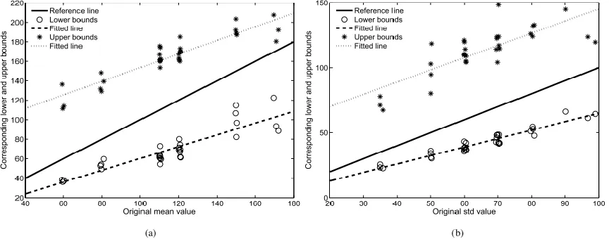
μe and σe are only rough estimates of the desired μ and σ values. For each LDR image, there should be certain ranges of μ and σ values surrounding μe and σe, within which the naturalness of the image is not degraded. To verify this and to provide a quantitative model, we conducted a subjective experiment, in which observers were asked to gradually decrease and then increase μ of the test LDR images until they saw significant degradation in

naturalness. A lower bound μl and a upper bound μr for each LDR image were thus recorded. The same procedure is used to obtain a lower std bound σl and a upper std bound σr for each LDR image. We selected 60 natural LDR images from the LIVE database [29] with different μ and σ values that cover diverse natural contents. A total of 25 naive observers, including 15 males and 10 females aged between 22 and 30, participated in the experiment. The four bounds for each LDR image are averaged over all 25 observers. Fig. 2 summarizes the experimental results, where we observe that the relationships between μ and the values of μl and μr are approximately linear. This motivates us to fit two linear models to predict μl and μr on the basis ofμ. The fitted models have slopes k1=0.60,k2=0.70 and interceptsb1=−0.14,b2=83.61 for μl and μr, respectively. The R 2 statistics of the two linear models are 0.8008 and 0.8465 respectively, which indicate that the linear models explain most variances in the subjective data. Perhaps the most interesting finding in this experiment is when μof an image is relatively small, μr –μ is much large than μ−μl. By contrast, the situation is reversed when μ of an image is large. In words, the acceptable luminance changes without significantly tampering an image‟s visual naturalness

Fig. 2. Subjective experiment results on the naturalness of mean and std values. The asterisks in (a) and (b) represent the upper bounds, given by the average subject, of the mean and std of test images, respectively. The corresponding

dotted lines are lease square fitted lines. The circles in (a) and (b) represent the lower bounds, given by the average subject, of the mean and std of test images, respectively. The corresponding dashed lines are lease square fitted

saturate at both small and large luminance levels. Similarly, σl and σr of a test LDR image can also be fitted by two linear models using σ as the predictor. The fitted lines for σl and σr have slopesk3=0.65,k4=0.94 and interceptsb3=−0.08, b4=51.40, respectively.

Based on the method described above, given an HDR image, we first estimate μe and σe and then predict μl , μr, σl and σr of the tone mapped image. The μ and σ values of a natural looking tone mapped image should at least fall in [μl,μr]and [σl,σr], and if possible, close to μe and σe. We quantify the drop from μe and σe to their lower and upper bounds using Gaussian cumulative distribution functions (CDF). Specifically, the likelihood of a tone mapped image to be natural given its mean μ is computed by

Where τ1 and θ1 are uniquely determined by two points (μl,0.01) and (μe,1) on the Gaussian CDF curve.

Correspondingly,τ2 andθ2 are uniquely determined by two points (μr,0.01)and(μe,1)on the Gaussian CDF curve. Similarly, the likelihood of a tone mapped image to be natural given its std σ is computed by two points(μl,0.01) and (μe,1) on the Gaussian CDF curve. Correspondingly,τ2 andθ2 are uniquely determined by two points (μr,0.01)and(μe,1)on the Gaussian CDF curve. Similarly, the likelihood of a tone mapped image to be natural given its std σ is computed by

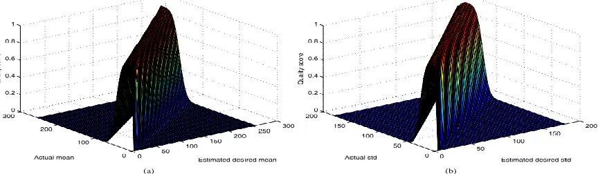
Where τ3 and θ3 are uniquely determined by two points (σl,0.01) and (σe,1) on the Gaussian CDF curve, and τ4 and θ4 are uniquely determined by two points (σr,0.01) and (σe,1) on the Gaussian CDF curve. The surfaces of Pm and Pd are plotted in Fig. 3.

It can be observed that μ and σ of the tone mapped image of high naturalness should be close to μe and σe, which correspond to the peaks along the diagonal lines.

Fig. 3. The surfaces of Pm and Pd in TMQI_II. (a) Pm(b) Pd. It suggests that the μ and σ of the natural looking tone mapped image should to close to μe and σe, which correspond to the peaks along the diagonal lines. The models

give heavy penalty when |μ−μe| or |σ−σe| is large.

It can be observed that μ and σ of the tone mapped image of high naturalness should be close to μe and σe, which correspond to the peaks along the diagonal lines. The models give heavy penalty when |μ−μe| or |σ−σe| is large.

Since 0≤Pm, Pd ≤1,N also lies in[0,1]. The superiority of the modified statistical naturalness term over that in TMQI is verified by improved correlation with respect to subjective evaluations as shown in Table I.

To continue with the iterative optimization procedure upon structural fidelity update, we start with the intermediate image ˆ Y k in Eq. (6) and improve the statistical naturalness to achieveYk+1through a three-segment equipartition monotonic piecewise linear function

This is essentially a point-wise intensity transformation with its parameters a and b(where 0 ≤a≤b≤L) chosen so that μ and σ ofYk+1 ={y i k+1 for all i} better approximate μe and σe of the desired tone mapped image.

To solve f or a and b, we first estimate the mean and std values ofYk+1 by

whereˆ μk and ˆ σk are the mean and std of ˆ Yk, respectively. λm and λd are step sizes that control the updating speed. Finding the parameters a and b is then converted to solving the following constrained optimization problem

Where η adjusts the weights between the mean and std terms. We adopt a standard gradient projection algorithm [30], [31] with a maximum of 30 iterations to solve this problem. Once the optimal values of a and b are obtained, they are plugged into (32) to create the resulting imageYk+1,which is subsequently fed into the (k+1)-th iteration.

TABLE I

PERFORMANCE EVALUATION OF THE STRUCTURAL FIDELITY AND STATISTICAL NATURALNESS TERMS IN TMQI AND TMQI-IION THE DATABASE[19]

The only difference lies in Eq. (33), where μe and σe are replaced with two constants corresponding to the peaks of fixed Pm and Pd models in TMQI.

We have five free parameters in the proposed algorithm. For fair comparison between TMQI and TMQI-II, we use the same set of parameters in all experiments, which are =0.1,λ=0.3,λm=λd =0.03 and η=1, respectively. A by-product of the above derivation of the iterative TMO algorithm is a renewed index, TMQI-II, given by

A by-product of the above derivation of the iterative TMO algorithm is a renewed index, TMQI-II, given by where both S and N measures have been improved upon those in TMQI. A number of parameters are inherited from TMQI. These includeC1 =0.01,C2 =10 and the threshold of the contrast visibility for tone mapped images τσ =2.6303. Throughout our study, we set the threshold of contrast visibility for HDR images τσ =0.06 and k =0.12. As for the model parameters in TMQI-II, we set a =0.5,α=1 and β=1, which emphasize the equal importance between structural fidelity and statistical naturalness terms.

III. EXPERIMENTAL RESULTS

To fully demonstrate the potentials of the proposed iterative algorithm, we select a wide range of HDR images, containing both indoor and outdoor scenes, human and static objects, as well as day and night views. The initial images for this algorithm are also generated by many different TMOs, ranging from simple ones such as Gamma mapping (γ =2.2) and log-normal mapping to state-of-the-art ones such as Durand‟s method [32], Mantiuk‟s method [33], Drago‟s method [4] and Reinhard‟s method [3]. The last one is considered one of the best TMOs based on several independent subjective tests [12], [19].

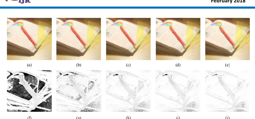
Fig. 4. Tone mapped “Desk” images and their structural fidelity maps. (a) Initial image created by Reinhard‟s algorithm [3]. (b)-(e) Images created using iterative structural fidelity update only. (f)-(j) Corresponding structural

fidelity maps of (a)-(e), where brighter indicates higher structural fidelity. All images are cropped for better visualization. (a) initial image (b) after 10 iterations (c) after 50 iterations (d) after 100 iterations (e) after 200 iterations (f) initial image, S =0.689 (g) 10 iterations, S=0.921 (h) 50 iterations, S=0.954 (i) 100 iterations, S=0.961

(j)200iterations,S=0.966.

Fig. 5. Tone mapped “Cornell box” images. (a) Initial image created by Gamma mapping (γ =2.2). (b)-(d) Images created using iterative statistical naturalness update only. (a) Initial image, N =0.000. (b) 10 iterations, N =0.0001.

(c) 30 iterations, N =0.0329. (d) 50 iterations, N =0.8355.(e) 100 iterations, N =0.9962.

In Fig. 5, the initial “Cornell box” image is created by the Gamma mapping (γ=2.2), and we apply the proposed iterative algorithm but using statistical naturalness updates only.

With the iterations, the overall brightness and contrast of the image are significantly improved, leading to a more visually appealing and natural-looking image. Table II lists the TMQI-II comparison between the initial images and the corresponding

optimization results on the “Woman” image initialized by Gamma mapping, which creates dark background with missing structures. Both TMQI and TMQI-II optimized images recover the structures of the background such as the white door, the yellow board and the photo frame, and present a better overall brightness. However, the TMQI optimized image suffers from heavy noise in homogenous areas such as in the wall and on the floor. The boosted noise artifact are likely due to the structural fidelity term in TMQI, which treats all local areas in the HDR image as contrast visible. In comparison, the TMQI-II optimized image is much cleaner and sharper. Fig. 7 shows the comparison of TMQI and TMQI-II optimization results on the “Clock building” image. The initial image created by log-normal mapping preservers most

structures but looks unrealistic due to its blanched appearance. This problem is largely alleviated in the TMQI-II optimized image, where the overall brightness and contrast of the image are significantly improved, leading to a more visually appealing and natural-looking image. By contrast, the TMQI optimized image suffers from excessive contrast between the lights and the bricks on the wall. This problem is likely rooted in its statistical naturalness term, which drags μ and σ of all tone mapped images towards 116 and 65 regardless of their contents and luminance levels [19]. This is inappropriate for a night scene like “Clock building” which desires lower μe and σe (In TMQI-II, μe =101 and σe =48). Moreover, annoying noise appears in the sky region of the TMQI optimized image.

TABLE II

Fig. 6. Tone mapped “Woman” images. (a) Initial image created by Gamma mapping. (b) TMQI optimized image. (c) TMQI-II optimized image

Fig. 6. Tone mapped “Woman” images. (a) Initial image created by Gamma mapping. (b) TMQI optimized image. (c) TMQI-II optimized image Fig. 8 shows the comparison of TMQI and TMQI-II optimization results on the “Bristol bridge” image with

Fig. 7. Tone mapped “Clock building” images. (a) Initial image created by log-normal mapping. (b) TMQI optimized image. (c) TMQI-II optimized image.

Fig. 8. Tone mapped “Bristol bridge” images. (a) Initial image created by Reinhard‟s method [3]. (b) TMQI optimized image. (c) TMQI-II optimized image.

Fig. 9. Tone mapped “Grove” images. (a) Initial image created by Drago‟s method [4]. (b) TMQI optimized image. (c) TMQI-II optimized image.

In Fig. 8(c), the proposed iterative algorithm using TMQI-II recovers these fine details and makes them much sharper. Moreover, the overall appearance is softer and thus more pleasant. In Fig. 8(b), we can see that the iterative algorithm using TMQI heavily boosts noise in the sky and cloud regions, which leads to quality degradation when compared with the initial

image. This also reveals the problem of TMQI in quality assessment of tone mapped images.

and sharpened. The overall appearance is also more vivid. However, in Fig. 9(b), the iterative algorithm using TMQI over stretches the global contrast, which

darkens the tree trunks and whitens the leafs and the sky. This affects the naturalness of the initial image and leads to quality degradation.

TABLE III

MEANOPINIONSCORES OFTONEMAPPEDIMAGES

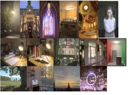
To further verify the effectiveness and consistency of the proposed algorithm, we conducted another subjective experiment. In particular, we select 15 HDR images that contain various natural scenes shown in Fig. 10 and adopt Gamma mapping, log-normal mapping and Reinhard‟s method [3] to tone-map them to 15×3=45 LDR images. We then use them as initial images of the iterative algorithm and obtain 45 TMQI optimized images and 45 TMQI-II optimized images, respectively. Eventually, we obtain 15 sets of tone mapped images, each of which contains 9 images. 24 naive subjects (9 males and 15 females aged between 22 and 30) were asked to give an integer score between 0 and 10 for the perceptual quality of each tone mapped image, where 0 denotes the worst quality and 10 the best. The final quality score for each individual image is computed as the average of subjective scores, named mean opinion score (MOS), from all subjects. The results are listed in Table III, from which we have several interesting observations. First, using TMQI-II as the optimization goal, the proposed algorithm leads to consistently perceptual

gain for all three different types of initial images. By contrast, the perceptual gain obtained by optimizing TMQI is much less, when initial images are created by Gamma and log-normal mapping. Indeed, the quality of TMQI optimized images decreases when the initial images are created by Reinhard‟s method [3]. Second, the best quality image on average is TMQI-II optimized with the initial image created by Reinhard‟s method [3]. Note that because the image space is extremely complicated and the proposed algorithm can only guarantee to find a local optimum; thus better initial images often lead to better local optima, which correspondingly have better perceptual quality.

Fig. 10. HDR test images used in the subjective experiment. The images shown here are TMQI-II optimized with initial images created by Reinhard‟s

method [3] .

TABLE IV

STATISTICAL SIGNIFICANCE MATRIX BASED ON THE HYPOTHESIS TESTING.“1”MEANS THAT THE ROW CATEGORYIS STATISTICALLY BETTER THAN THE COLUMN CATEGORY.“0”MEANS THAT THE

COLUMN CATEGORY IS STATISTICALLY BETTER THAN THEROW CATEGORY. “MEANS THAT THE ROW AND COLUMN CATEGORIES ARE STATISTICALLY INDISTINGUISHABLE. G:GAMMAMAPPING INITIALIZED;L:LOG NORMAL MAPPING INITIALIZED;R:REIN HARD‟SMETHOD[3] INITIALIZED; (I):

TMQI OPTIMIZED AND(II): TMQI-II OPTIMIZED

Specifically, we treat the MOS values of each column in Table III as one category. The null hypothesis is that the MOS values in one category is statistically indistinguishable (with 95% confidence) from those in another category. The test is carried out for all possible combinations of pairs of categories, and the results are summarized in Table IV, from which we can see that TMQI-II optimized images have statistically significantly better MOS values in all cases.

In summary, we believe that the proposed iterative optimization procedure provides a strong test

that not only verifies the superiority of TMQI-II over TMQI in predicting the perceptual quality of tone mapped images but also shows that the robustness and usefulness of TMQI-II to guide the optimization process with a variety of initial images.

different initial images as the starting points. There are several useful observations. First, both measures increase monotonically with iterations. Second, the proposed algorithm converges in all cases regardless of using simple or sophisticated TMO results as initial images. Third, different initial images may result in different converged images. From these observations, we conclude that the proposed iterative algorithm is well behaved, but the high-dimensional search space is complex and contains many local optima, and the proposed algorithm may be trapped in one of them.

The computation complexity of the proposed algorithm increases linearly with the number of pixels in the image. Our un optimized MATLAB implementation takes around 4 seconds per iteration for a 341×512 image on a computer with an Intel Quad-Core 2.67 GHz processor.

Fig. 11. Structural fidelity as a function of iteration with initial “woods” images created by different TMOs

Fig. 12. Statistical naturalness as a function of iteration with initial “woods” images created by different TMOs

IV. CONCLUSION AND FUTURE WORKS

We propose a novel approach to design TMOs by navigating in the space of images to find the optimal image in terms of an improved TMQI or TMQI-II. TMQI-II overcomes the limitations underlying the structural fidelity and statistical naturalness components in TMQI and thus has better correlation with subjective quality evaluation. Optimizing TMQI-II is based on an iterative approach that alternates between improving the structural fidelity preservation and enhancing the statistical naturalness of the image. Numerical and subjective experimental results show that both steps contribute significantly to the improvement of the overall quality of the tone mapped image. The proposed algorithm further verifies the superiority of TMQI-II over TMQI. Finally, our experiments show that the proposed method is well behaved, and effectively enhances image quality from a wide variety of initial images, including those created from state-of-the-art TMOs.

The current work opens the door to a new class of tone mapping approaches. Many topics are worth further investigations. First, as is the case for any algorithm operating in complex high-dimensional spaces, the current approach only finds local optima. Deeper understanding of the search space is desirable to better solve the optimization problem. Second, the current implementation is computationally costly and requires a large number of iterations to converge. Fast search algorithms are necessary to accelerate the iterations. Third, objective quality assessment of tone mapped images still has much space to improve. In the future, better objective IQA models may be incorporated into the proposed framework to create better quality tone mapped images.

REFERENCES

[2] E. Reinhard, W. Heidrich, P. Debevec, S. Pattanaik, G. Ward, and K. Myszkowski,High Dynamic Range Imaging: Acquisition, Display, and Image-Based Lighting. San Mateo, CA, USA: Morgan Kaufmann, 2010.

[3] E. Reinhard, M. Stark, P. Shirley, and J. Ferwerda, “Photographic tone reproduction for digital images,” ACM Trans. Graph., vol. 21, no. 3, pp. 267–276, 2002.

[4] F. Drago, K. Myszkowski, T. Annen, and N. Chiba, “Adaptive logarithmic mapping for displaying high contrast scenes,” Comput. Graph. For um, vol. 22, no. 3, pp. 419–426, 2003.

[5] Q. Shan, J. Jia, and M. S. Brown, “Globally optimized linear windowed tone mapping,” IEEE Trans. Vis. Comput. Graphics, vol. 16, no. 4, pp. 663– 675, Jul./Aug. 2010.

[6] S. Ferradans, M. Bertalmio, E. Provenzi, and V. Caselles, “An analysis of visual adaptation and contrast perception for tone mapping,”IEEE Trans. Pattern Anal. Mach. Intell., vol. 33, no. 10, pp. 2002–2012, Oct. 2011.

[7] B. Gu, W. Li, M. Zhu, and M. Wang, “Local edge-preserving multiscale decomposition for high dynamic range image tone mapping,” IEEE Trans. Image Process., vol. 22, no. 1, pp. 70–79, Jan. 2013.

[8] H. Yeganeh and Z. Wang, “High dynamic range image tone mapping by maximizing a structural fidelity measure,” inProc. IEEE Int. Conf. Acoust., Speech Signal Process., May 2013, pp. 1879–1883.

[9] K. Ma, H. Yeganeh, K. Zeng, and Z. Wang, “High dynamic range image tone mapping by optimizing tone mapped image quality index,” in Proc. IEEE Int. Conf. Multimedia Expo, Jul. 2014, pp. 1–6.

[10] F. Drago, W. L. Martens, K. Myszkowski, and H.-P. Seidel, “Perceptual evaluation of tone mapping operators,” in Proc. ACM SIGGRAPH Sketches Appl., 2003, p. 1.

[11] M. ˇ Cadík and P. Slavík, “The naturalness of reproduced high dynamic range images,” in Proc. 9th Int. Conf. Inf. Vis., 2005, pp. 920–925.

[12] M. ˇ Cadík, M. Wimmer, L. Neumann, and A. Artusi, “Evaluation of HDR tone mapping methods using essential perceptual attributes,” Comput. Graph., vol. 32, no. 3, pp. 330–349, 2008.

[13] C. Cavaro-Ménard, L. Zhang, and P. Le Callet, “Diagnostic quality assessment of medical images: Challenges and trends,” inProc. IEEE 2nd Eur. Workshop Vis. Inf. Process., Jul. 2010, pp. 277–284.

[14] Z. Wang, A. Bovik, H. Sheikh, and E. Simoncelli, Image quality assessment: From error visibility to structural similarity, IEEE Trans. Img. Proc., vol. 13, no. 4, pp. 600C612, 2004.

[15] Z. Wang, A. C. Bovik, H. R. Sheikh, and E. P. Simoncelli, “Image quality assessment: From error visibility to structural similarity,”IEEE Trans. Image Process., vol. 13, no. 4, pp. 600–612, Apr. 2004.

[16] J. Preiss, F. Fernandes, and P. Urban, Color-image quality assessment: From prediction to optimization, IEEE Trans. Img. Proc., vol. 23, no. 3, pp. 1366C1378, 2014.

[17] Soundararajan, Rajiv, and A. C. Bovik, RRED indices: Reduced reference entropic differencing for image quality assessment, IEEE Trans. Img. Proc., vol. 21, no. 2, pp. 517C526, 2012.

[18] T. O. Aydin, R. Mantiuk, K. Myszkowski, and H.-P. Seidel, “Dynamic range independent image quality assessment,” ACM Trans. Graph., vol. 27, no. 3, 2008, Art. ID 69.

[19] A. Rehman and Z. Wang, Reduced-reference image quality assessmentby structural similarity estimation, IEEE Trans. Img. Proc., vol. 21, no. 8,pp. 3378C3389, 2012.

[20] K. Gu, G. Zhai, X. Yang, and W. Zhang, Using free energy principlefor blind image quality assessmen, IEEE Trans. Multimedia, vol. 17, no.1, pp. 50 C 63, 2015.

[22] Q. Li, W. Lin, and Y. Fang, No-reference quality assessment formultiply-distorted images in gradient domain, IEEE Signal Process. Lett.,vol. 23, no. 4, pp. 541 C 545, 2016..

[23] Z. Wang and E. P. Simoncelli, “Stimulus synthesis for efficient evaluation and refinement of perceptual image quality metrics,”Proc. SPIE, vol. 5292, pp. 99– 108, Jun. 2004.

[24] Z. Wang and E. P. Simoncelli, “Maximum differentiation (MAD) competition: A methodology for comparing computational models of perceptual quantities,”J. Vis., vol. 8, no. 12, p. 8, 2008.

[25] G. Ward, “A contrast-based scalefactor for luminance display,” inGraphicsGemsIV, P. Heckbert, Ed. San Diego, CA, USA: Academic, 1994, pp. 415– 421.

[26] J. Holm, “Photographic toneand color reproduction goals,” inProc. CIE Expert Symp., Color Standards Image Technol., 1996, pp. 51–56.

[27] N. Salvaggio, L. Stroebel, and R. Zakia, Basic Photographic Materials and Processes. New York, NY, USA: Taylor & Francis, 2008.

[28] Y. Li, L. Sharan, and E. H. Adelson, “Compressing and companding high dynamic range images with subband architectures,” ACM Trans. Graph., vol. 24, no. 3, pp. 836–844, 2005.

[29] H. R. Sheikh, Z. Wang, L. Cormack, and A. C. Bovik. Live Image Quality Assessment Database.

[Online]. Available: http://

live.ece.utexas.edu/research/quality, accessed Nov. 2006.

[30] S. P. Boyd and L. Vandenberghe, Convex Optimization. Cambridge, U.K.: Cambridge Univ. Press, 2004.

[31] J. Nocedal and S. J. Wright,Numerical Optimization, 2nd ed. New York, NY, USA: Springer-Verlag, 2006.

[32] F. Durand and J. Dorsey, “Fast bilateral filtering for the display of highdynamic-range images,”ACM Trans. Graph., vol. 21, no. 3, pp. 257–266, 2002.

[33] R. Mantiuk, S. Daly, and L. Kerofsky, “Display adaptive tone mapping,” ACM Trans. Graph., vol. 27, no. 3, 2008, Art. ID 68.