Abstract
PETERSEN, RICHARD FRANCIS. Transformation Semigroups Over Groups. (Under the direction of Mohan Putcha.)
The semigroup analogue of the symmetric group, Sn, is the full transfor-mation semigroup, Tn. Tn is the set of all mappings from the set {1,2, ..., n} to itself. This semigroup has been studied in great detail, especially in con-nection with automata theory.
The wreath product of a group G bySn has been studied for almost one hundred years. In this thesis, we study the wreath product of a group Gby Tn. These wreath products are expressed asGwrSnandGwrTn, respectively. Many interesting theorems and properties for wreath products will be dis-cussed. For example, the result of John Howie that every element inTn−Sn can be expressed as a product of idempotents, is generalized to show that any element of GwrTn−GwrSn can be expressed as a product of idempotents. It will also be shown that GwrTn is unit regular.
conju-Transformation Semigroups Over Groups
by
Richard F. Petersen
A dissertation submitted to the Graduate Faculty of North Carolina State University
in partial fulfillment of the requirements for the Degree of
Doctor of Philosophy
Mathematics
Raleigh, North Carolina 2008
APPROVED BY:
Dr. Mohan Putcha Dr. Kailash Misra Chair of Advisory Committe
Dedication
Biography
Richard F. Petersen was born March 6, 1979 in Lowell, MA. He attended elementary schools in California, New York, and Massachusetts. Afterwards, he attended junior high and high schools in Michigan and New Jersey. In 1997, he graduated with honors from Pemberton Township High School in Pemberton,NJ.
In 1999, Richard obtained an Associate of Science in Liberal Arts and Sciences from Burlington County College in Pemberton,NJ. He went on to attend Elizabeth City State University in Elizabeth City, NC where he earned a Bachelor of Science in Mathematics in 2002. While at ECSU, he worked on a research project on chaos in communication systems with Dr. Dipendra Sengupta. During the summer of 2002, the late Dr. Georgia Lawrence hired Richard to teach his first mathematics course, at ECSU.
Acknowledgements
I would like to thank God for everything. I would like to thank my advisor, Dr. Mohan Putcha, for the many hours he spent guiding me in my research and in my career. I would like to thank my parents: Rick Petersen and Karen Petersen, my grandparents: Frank McNanley, Hilda McNanley, Dick Petersen, and Marcia Petersen, my brother: Andrew Petersen, and my aunts, uncles and cousins for their many years of support and guidance.
I would like to thank the following friends who have made this long journey bearable:
Table Of Contents
List of Tables. . . .ix
1 - Groups . . . 1
1.1 - Basic Definitions . . . 1
1.2 - Group Examples . . . 2
1.3 - Focusing On Sn and Sfn. . . 3
1.4 - Notation . . . 3
1.4.1 - Two Line Notation . . . 3
1.4.2 - One Line Notation . . . 4
1.4.3 - Cycle Notation . . . 4
1.4.4 - Matrix Notation . . . 5
1.4.5 - Directed Graph Notation . . . 6
1.5 - Conjugacy Classes In Sn. . . 7
1.6 - Looking Ahead To Chapter 2 . . . 8
2 - Semigroups . . . 9
2.1 - Basic Definitions . . . 9
2.2 - Semigroup Examples . . . 10
2.3 - Notation. . . .11
2.3.2 - One Line Notation . . . 11
2.3.3 - Matrix Notation . . . 11
2.3.4 - Directed Graph Notation . . . 12
2.4 - Orders of Full Transformation Semigroups . . . 12
2.5 - Regular Semigroups . . . 13
2.6 - Rank and Range of Elements in Tn. . . 14
2.7 - Idempotents in Tn and Tfn. . . .14
2.8 - Looking Ahead To Chapters 3 and 4 . . . 17
3 - The Wreath Product GwrSn. . . 18
3.1 - Defining GwrSn. . . 18
3.2 - GwrSn Is A Group . . . 18
3.3 - Notation and Examples . . . 19
3.4 - Multiplication of Elements in GwrSn. . . 21
4 - The Wreath Product GwrTn. . . 23
4.1 - Defining GwrTn. . . 23
4.2 - GwrTn Is A Monoid . . . 23
4.3 - Notation and Examples . . . 24
4.4 - Multiplication Of Elements In GwrTn. . . 26
4.5 - GwrTn Is Unit Regular . . . 27
5.1 - Green’s Relations On A Monoid M. . . 33
5.2 - Green’s Relations For Idempotents . . . 34
5.3 - Green’s Relations For Tn. . . .34
5.4 - Green’s Relations For Idempotents In GwrTn. . . 39
5.5 - Looking Ahead To Chapter 6 . . . 44
6 - Conjugacy Classes inSn and Tn. . . 45
6.1 - Conjugacy Classes Of Sn Revisited. . . .45
6.2 - Conjugacy Classes Of Tn. . . 46
6.2.1 - The Conjugacy Classes Of T1 and T2. . . 49
6.2.2 - The Conjugacy Classes Of T3. . . 51
6.2.3 - The Conjugacy Classes Of T4. . . 53
6.2.4 - More About Generalized The Cycle Structure . . . 61
7 - Conjugacy Classes inGwrSn. . . 63
7.1 - N-Cycles In GwrSn. . . 63
7.2 - Example In GwrS12. . . 66
7.3 - The Conjugacy Class Formula For GwrSn. . . 67
8 - Conjugacy Classes inGwrTn. . . .72
8.1 - Conjugation Examples . . . 72
8.2 - The Two Lemmas . . . 76
8.3 - The Conjugacy Class Formula For GwrTn . . . 79
List of Tables
Table 5.3.1 - D1-class of T3. . . 35
Table 5.3.2 - D2-class of T3. . . 35
Table 5.3.3 - D3-class of T3. . . 35
Table 5.3.4 - Eggbox Diagram for T3 . . . 36
Table 5.3.5 - D1-class of Tf3. . . 37
Table 5.3.6 - D2-class of Tf3. . . 38
1
Groups
It is necessary to review a bit of group theory before proceeding on to the new material in this thesis. The following definitions will be useful to keep in mind.
1.1
Basic Definitions
Definition 1.1.1 A group is a set G together with a law of composition, * , which has the following properties: For a, b, c∈G,
(1) a∗(b∗c) = (a∗b)∗c (associativity) (2) 1∈G (identity)
(3) If a∈G, then a−1 ∈G (inverses)
If the law of composition, * , is commutative (i.e., a∗ b = b ∗ a, for a, b ∈ G), then G is said to be an Abelian group. We may also wish to consider special kinds of subsets of Gcalled subgroups.
Definition 1.1.2 A subgroup is a subset H of a group G which has the following properties, for a, b∈H,
(1) If a∈H and b ∈H, then a∗b∈H (closure under the operation *)
(2) 1∈H (identity element)
1.2
Group Examples
The following are classic examples of groups:
Example 1.2.1 General Linear Group
GLn = { n×n matrices A with det A6= 0}
Example 1.2.2 Special Linear Group
SLn = { n×n matrices B with det B = 1} SLn is a subgroup of GLn.
Example 1.2.3 Dihedral Group
Dn = group generated by two elements, x and y, such that the relations
xn= 1, y2 = 1, and yx=x−1y hold.
Example 1.2.4 Symmetric Group
Sn = the set of all bijections from {1,2, ..., n} → {1,2, ..., n}.
More generally, SX is the group of all permutations of any set X.
Example 1.2.5 Signed Permutation Group
f
Sn = the set of all bijections from {1,2, ..., n} → {±1,±2, ...,±n}.
Example 1.2.6 Weyl Groups
The group of type An−1 corresponds to the symmetric group, Sn, and the
1.3
Focusing on
S
nand
S
gn
The symmetric group, Sn, and the signed permutation group, Sfn, are of the
most importance for future chapters, so we shall focus on them in greater detail for the rest of this chapter. These results are well known and have appeared in numerous papers and books.
Definition 1.3.1 Theorder of a groupGis the number of elements in G. We denote the order of G by the symbol, |G|.
Theorem 1.3.2 |Sn|=n! Example 1.3.3 |S6|= 6! = 720
Corollary 1.3.4 |Sfn|= 2n·n!
Example 1.3.5 |Sf6|= 26(6!) = (64)(720) = 46,080
1.4
Notation
We have a few useful ways to represent elements in Sn. The following nota-tions will be used where appropriate.
1.4.1 Two Line Notation Letπ ∈Sn; we can write π=
1 2 3 · · · n π(1) π(2) π(3) · · · π(n)
!
.
1.4.2 One Line Notation
In two line notation, the top line is always the same, so we may omit it and just write the bottom line. Let π ∈Sn; we can write
π = π(1) π(2) π(3) · · · π(n) .
Example 1.4.2 If π∈S4 and π(1) = 4, π(2) = 2, π(3) = 1, π(4) = 3, then
π = 4 2 1 3 .
1.4.3 Cycle Notation
Sagan gives a nice description of this cycle notation in his book on the symmetric group [10]. Given i ∈ {1,2, ..., n}, the elements of the sequence i, π(i), π2(i), π3(i), ... cannot all be distinct. Taking the first power p, such
that πp(i) = i, we have the cycle i π(i) π2(i) · · · πp−1(i) .
Equiva-lently, the cycle i j k · · · l means thatπ sendsitoj,j tok, ..., and l back toi.
Example 1.4.3 If π∈S4 and π(1) = 4, π(2) = 2, π(3) = 1, π(4) = 3, then
π = (143)(2) in cycle notation.
Definition 1.4.4 A k-cycle, or cycle of length k, is a cycle containing
k elements.
Example 1.4.6 σ= (12)(34)(5678) consists of two cycles of length 2 and a cycle of length 4.
Definition 1.4.7 Thecycle type, or simply the type, of π is an expres-sion of the form 1m1 2m2 3m3 · · · nmn , where m
k is the number of
cycles of length k in π.
Example 1.4.8 π= (143)(2) has cycle type 11 20 31 40 .
Example 1.4.9 σ= (12)(34)(5678)has cycle type 10 22 30 41 50 60 70 80 .
Another way to give the cycle type is as a partition:
Definition 1.4.10 Apartition ofn is a sequenceλ = (λ1, λ2, ..., λl), where λi are weakly decreasing and
l
X
i=1
λi =n. Thus, k is repeated mk times in the
partition version of the cycle type of π.
Example 1.4.11 For π = (143)(2), λ= (3,1).
Example 1.4.12 For σ = (12)(34)(5678), λ = (4,2,2).
1.4.4 Matrix Notation
Let π ∈Sn; we can indicate π(j) = i by placing a 1 in the (i, j)-entry of an n×n matrix.
Example 1.4.13 π= (143)(2), which means π(1) = 4, π(2) = 2, π(3) = 1,
π(4) = 3, can be written in matrix notation as π =
0 0 1 0 0 1 0 0
1.4.5 Directed Graph Notation
Consider an elementπ ∈Sn, whereπ= i j k · · · l in cycle notation. Draw n vertices and label them i, j,k, ..., l. Indicateπ(i) =j by drawing a directed line segment from i toj.
Example 1.4.14 For π = (143)(2) the directed graph is,
1
= = = = = = = 2ee
3
O
O
4
o
o
Each of these four notations will be used throughout this thesis. Later on, some variations of these notations will be used.
Example 1.4.15 Similar notation works for elements in Sfn.
If π = 1 2 3 4
−2 4 −1 3
!
∈ Sf4, we can represent this element in matrix
form by placing ±1 in the (i, j)-entry to indicate j → ±i.
So, π=
0 0 −1 0
−1 0 0 0
0 0 0 1
0 1 0 0
.
We can also make a slight modification on our directed graph notation to
represent π as
1 −1 //2
1
3
−1
O
O
4
1
o
1.5
Conjugacy Classes In
S
nDefinition 1.5.1 In any group G, elements g and h are conjugates if
g =khk−1, for some k∈G.
Definition 1.5.2 The set of all elements conjugate to a given g ∈ G is called the conjugacy class of g.
In Sn, if π = i1 i2 i3 · · · il im im+1 im+2 · · · in
in cycle notation, then for any σ ∈Sn,
σπσ−1 = σ(i
1) σ(i2) σ(i3) · · · σ(il) σ(im) σ(im+1) σ(im+2) · · · σ(in)
.
Conjugacy is an equivalence relation, so the distinct conjugacy classes partition G. This means that if G has t conjugacy classes, C1, C2, ..., Ct, then Ci∩Cj =∅, fori6=j, and [
i
Ci =G.
Example 1.5.3 We can write the number 1 only as 1, so S1 has only 1
conjugacy class.
We can write the number2 as2 + 0 and 1 + 1, so S2 has 2conjugacy classes.
We can write the number3as 3 + 0, 2 + 1 and1 + 1 + 1, soS3 has3conjugacy
classes.
We can write the number 4 as 4 + 0, 3 + 1, 2 + 2, 1 + 1 + 2 and 1 + 1 + 1 + 1, so S4 has 5 conjugacy classes.
We can write the number 5 as 5 + 0, 1 + 4, 2 + 3, 1 + 1 + 3, 1 + 2 + 2,
1 + 1 + 1 + 2, and 1 + 1 + 1 + 1 + 1, so S5 has 7 conjugacy classes.
We will consider the conjugacy classes of Sfn in a later chapter. See the
chapters on conjugacy classes in wreath products for those results.
1.6
Looking Ahead To Chapter 2
2
Semigroups
In this chapter we will examine numerous properties and examples of semi-groups. We begin with the following well known definitions.
2.1
Basic Definitions
Definition 2.1.1 Amonoidis a setM together with a law of composition, *, which has the following properties: For a, b, c∈M,
(1) a∗(b∗c) = (a∗b)∗c (associativity) (2) 1∈M (identity)
Definition 2.1.2 A semigroup is a set S together with a law of composi-tion, *, which is associative.
Definition 2.1.3 Let S be a semigroup and T ⊆S. T is a subsemigroup, if T is closed under the semigroup operation, *.
Definition 2.1.4 Let S be a semigroup. We say an element, σ ∈ S, is
idempotent if and only if σ2 =σ. We denote the set of all idempotents in
S by E(S).
2.2
Semigroup Examples
Example 2.2.1 The set of all integers,Z, under multiplication, is a monoid.
Example 2.2.2
The set of all positive integers, under addition, is a semigroup.
Example 2.2.3
The set of all nonnegative matrices, under matrix multiplication, is
a semigroup.
Example 2.2.4 Full Transformation Semigroup
Tn = the set of all mappings from {1,2, ..., n} → {1,2, ..., n}.
Tn is the semigroup analogue of Sn. We notice that Sn is the unit group of
Tn.
Example 2.2.5 Signed Full Transformation Semigroup
f
Tn = the set of all mappings from {1,2, ..., n} → {±1,±2, ...,±n}.
f
Tn is the semigroup analogue of Sfn. We see that Sfn is the unit group of Tfn.
2.3
Notation
The following notations are of the most use for representing elements in full transformation semigroups. These notations should look similar to those used in the last chapter.
2.3.1 Two Line Notation Letπ ∈Tn. We can write π=
1 2 3 · · · n
π(1) π(2) π(3) · · · π(n)
!
.
Example 2.3.1 If π ∈ T5 and π(1) = 1, π(2) = 1, π(3) = 4, π(4) = 4,
π(5) = 5, then π = 1 2 3 4 5 1 1 4 4 5
!
.
2.3.2 One Line Notation
Once again, we may remove the top line in the two line notation to get π = π(1) π(2) π(3) · · · π(n) .
Example 2.3.2 If π ∈ T5 and π(1) = 1, π(2) = 1, π(3) = 4, π(4) = 4,
π(5) = 5, then π = 1 1 4 4 5 .
2.3.3 Matrix Notation
Example 2.3.3 π= (11445)∈T5, which means π(1) = 1, π(2) = 1,
π(3) = 4, π(4) = 4, π(5) = 5, can be written in matrix notation as
π =
1 1 0 0 0 0 0 0 0 0 0 0 0 0 0 0 0 1 1 0 0 0 0 0 1
.
2.3.4 Directed Graph Notation Consider an element π ∈ Tn, where π =
i j k · · · l in one-line no-tation. Draw n vertices and label them i, j, k, ..., l. Indicate π(i) = j by drawing a directed line segment from i to j.
Example 2.3.4 For π = (1111)∈T4, the directed graph is,
1
%
%
2
o
o
3
O
O
4
^
^
=== ====
2.4
Orders of Full Transformation Semigroups
Definition 2.4.1 The order of a semigroup S is the number of elements in S. We denote the order of S by the symbol, |S|.
Theorem 2.4.2 |Tn|=nn
Example 2.4.3 |T6|= 66 = 46,656
Corollary 2.4.4 |Tfn|= 2n·nn= (2n)n
2.5
Regular Semigroups
Definition 2.5.1 An element y of a semigroup S is called regular if there exists x∈S, such that yxy =y.
Definition 2.5.2 A semigroup S is called a regular semigroup if all of its elements are regular.
Definition 2.5.3 A semigroup is said to be unit regular if for each y∈S
there is a unit u such that yuy=y.
Theorem 2.5.4 Tn is a regular semigroup.
Proof:
(This proof comes from [9].) For everyα∈Tn, it is easily seen that the rela-tionshipyxy =y holds for every x∈Tn, such thatx(α) (α∈ {1,2, ..., n}) is equal to some one of the elements β, for which y(β) =α and arbitrarily, for
α6∈y({1,2, ..., n}). 2
Theorem 2.5.5 Tfn is a regular semigroup.
2.6
Rank and Range of Elements in
T
nDefinition 2.6.1 Let nˆ={1,2, ..., n}and σ∈Tn. Therangeofσ, denoted
Rng(σ), is σ(ˆn).
Definition 2.6.2 Let nˆ={1,2, ..., n} and σ ∈Tn. The rank of σ, denoted
Rnk(σ), is |σ(ˆn)|.
Example 2.6.3 Consider the elements (111), (122), and (123) from T3.
Rng((111)) ={1}, Rng((122)) ={1,2}, and Rng((123)) ={1,2,3}.
Example 2.6.4 Once again, consider the elements (111), (122), and (123)
from T3. Rnk((111)) = 1, Rnk((122)) = 2, and Rnk((123)) = 3. We see
that the ranks of the elements are just the orders of the sets from the above
example. Another way to find the rank is by writing the elements in matrix
form and using techniques from linear algebra.
2.7
Idempotents in
T
nand
T
gn
Definition 2.7.1 We say an element σ ∈ Tn is idempotent if and only
if σ2 =σ. We denote the set of all idempotents in T
n by E(Tn).
Example 2.7.2 Consider the element (223) ∈ T3. We can write this
ele-ment in matrix form as,
0 0 0 1 1 0 0 0 1
.
We can see this element is idempotent via matrix multiplication,
0 0 0 1 1 0 0 0 1
0 0 0 1 1 0 0 0 1
=
0 0 0 1 1 0 0 0 1
We could also see that Rng((223)) ={2,3}, and we do in fact have e(2) = 2
and e(3) = 3. So, our alternate definition for idempotent elements is also
satisfied in this case.
Example 2.7.3 Some other idempotents in T3 are:
(1) The element,(111), which we can write in matrix form as,
1 1 1 0 0 0 0 0 0
.
(2) The element,(122), which we can write in matrix form as,
1 0 0 0 1 1 0 0 0
.
(3) The element,(121), which we can write in matrix form as,
1 0 1 0 1 0 0 0 0
.
Example 2.7.4 ForT2, the set of all idempotent elements isE(T2) ={(11),(22),(12)},
Example 2.7.5 For Tf2, the set of all idempotent elements is
E(Tf2) = {(1 1),(2 2),(1 2),(1−1),(−2 2)}, where elements are written in one
line notation.
Example 2.7.6 For T3, the set of all idempotent elements is
E(T3) = {(111),(222),(333),(123),(113),(121),(122),(133),(223),(323)}, where
elements are written in one line notation.
In 1966, John M. Howie proved that the subsemigroupTn−Snis generated by the idempotents ofTn. The following is a rewording of the theorem in [6].
Theorem 2.7.7 Every element of Tn−Sn can be expressed as a product of
idempotent elements.
The proof of this theorem may be found in [6] on pages 708-709. He proves the theorem using notation that is not found in this thesis. Therefore, it is left to the interested reader to sort through Howie’s proof.
Example 2.7.8 In T3, we can write the non-idempotent,
0 0 0 1 0 0 0 1 1
, as a
product of idempotents in the following way:
0 0 0 1 0 0 0 1 1
=
0 0 0 1 1 0 0 0 1
1 0 0 0 0 0 0 1 1
It is also possible to express every element in Tfn−Sfn as a product of
idempotents. This result will be proved in Chapter 4. It is a special case of a theorem about the idempotents of wreath products.
Example 2.7.9 In Tf3, we can write the non-idempotent,
−1 1 1
0 0 0
0 0 0
, as
a product of idempotents in the following way:
−1 1 1
0 0 0
0 0 0
=
1 −1 −1
0 0 0
0 0 0
0 0 0 0 0 0 1 1 1
1 −1 −1
0 0 0
0 0 0
2.8
Looking Ahead To Chapters 3 and 4
In the next two chapters, we will work with the wreath products of a group G by the symmetric group Sn and a group G by the full transformation semigroup Tn. We will see how to constructSfn and Tfn via wreath products.
3
The Wreath Product
GwrS
nWe will show many interesting properties ofGwrSnin this chapter. First, we will constructGwrSn and show that it is a group. We follow the exposition in [8].
3.1
Defining
GwrS
nConsider a group Gand let ˆn={1,2, ..., n}. The product of G with itselfn times, G×G× · · · ×G, will be denoted Gˆn. Gˆn is the set of all mappings from ˆn intoG. In other words, Gˆn={f|f : ˆn→G}.
We put GwrSn=Gnˆ×Sn ={(f, π)|f : ˆn →G, π∈Sn} and, for f ∈Gnˆ and π ∈ Sn, we define fπ = f ◦ π. We define a multiplication on Gnˆ as follows: For f, f0 ∈ Gnˆ, (f f0)(i) = f(i)f0(i), where i ∈ ˆn. Using this, we define a law of composition on GwrSn,
(f, π)(f0, π0) = (fπ0f0, ππ0) = ((f◦π0)f0, ππ0)
3.2
GwrS
nIs A Group
If we define e ∈ Gnˆ by e(i) = 1G, where i ∈ ˆn, then the identity element of GwrSn will be 1GwrSn = (e,1Sn). For f ∈ G
ˆ
n, the mapping f−1 ∈ Gnˆ is
defined by f−1(i) = (f(i))−1, for i ∈ ˆn. Using this, we define the inverse of
(f, π)∈GwrSn to be (f, π)−1 = (fπ−1, π−1) = (f−1◦π−1, π−1).
element, (f, π)∈GwrSn, has an inverse element, (f, π)−1 ∈GwrSn.
For elements (f, π),(g, σ),(h, γ)∈GwrSn, it can be shown, with a little work, that (f, π)[(g, σ)(h, γ)] = [(f, π)(g, σ)](h, γ). Therefore, the law of composition for GwrSn is associative. This shows us that GwrSn forms a group, called the wreath product of G by Sn, using the given law of composition.
Since GwrSn is a group, it can also be shown that
[(f, π)(g, σ)]−1 = (g, σ)−1(f, π)−1, where (f, π),(g, σ) ∈ GwrSn. The order of GwrSn is |GwrSn|=|G|n· |Sn|=|G|n·n!, if Gis finite.
3.3
Notation and Examples
Example 3.3.1 Z2wrSnis the wreath product of the group of sign changes by Sn. This is just the set of all bijections from{1,2, ..., n} → {±1,±2, ...,±n}.
So, Z2wrSn =Snf. In Chapter 1, we claimed that |Sn|f = 2n·n!. We see this
is the case in another way, |Z2wrSn|=|Z2|n· |Sn|= 2n·n!.
Example 3.3.2 We see that Z2wrS2 =
n 1 0
0 1
!
, 1 0 0 −1
!
,
−1 0
0 1
!
, −1 0
0 −1
!
, 0 1 1 0
!
, 0 −1
1 0
!
, 0 1
−1 0
!
, 0 −1
−1 0
! o
We can represent the elements in GwrSn in a few different ways. Vari-ations on the previous graph notation and matrix notation will be of the greatest use in this chapter.
Example 3.3.3 Consider GwrS3 and let g1, g2, g3 ∈ G. We can represent
the mapping, 1−→g1 3, 2−→g3 1, 3−→g2 2, by a graph,
1 g1 2 g3 o o 3 g2 @ @
or as a matrix,
0 g3 0
0 0 g2
g1 0 0
,
where j −→g i is represented by placing g ∈G in the (i, j)-entry of the n×n matrix.
Example 3.3.4 Consider GwrS5 and let h ∈ G. We can represent the
mapping, 1−→h 2, 2−→h 1, 3−→h 3, 4−→h 5, 5−→h 4, by a graph,
1 h ((
2 h
h
h
3 h %%
4 h ((5 h
h
h
or as a matrix,
0 h 0 0 0
h 0 0 0 0
0 0 h 0 0
0 0 0 0 h
0 0 0 h 0
Example 3.3.5 Consider KwrS4 and let k1, k3, k4, k5 ∈K. We can
repre-sent the mapping, 1 k1
−→1, 2 k3
−→3, 3 k4
−→4, 4 k5
−→2, by a graph,
1 k1
%
%
2 k3
3 k4
/
/4
k5
O
O
or as a matrix,
k1 0 0 0
0 0 0 k5
0 k3 0 0
0 0 k4 0
.
We may also use wreath product notation to define the following: ˆ
S ={(1, π)|π ∈Sn} ∼=Sn and ˆ
G={(f,1)|f ∈Gˆn} ∼=Gnˆ ∼=G×G×G× · · · ×G.
3.4
Multiplication of Elements in
GwrS
nWe can think of multiplication of elements in GwrSn in a couple of different ways:
(1) i←−g j g
0
←−k, whereg, g0 ∈G.
Example 3.4.1 In GwrS3, let g1, g2, g3 ∈ G and consider two elements,
z, z0 ∈GwrS3, where
z : 1−→g1 2, 2 −→g2 3, 3−→g3 1, is represented by the matrix,
0 0 g3
g1 0 0
0 g2 0
,
and
z0 : 1−→g3 1, 2−→g2 3, 3−→g1 2, is represented by the matrix,
g3 0 0
0 0 g1
0 g2 0
.
Then, zz0 =
0 0 g3
g1 0 0
0 g2 0
g3 0 0
0 0 g1
0 g2 0
=
0 g3g2 0
g1g3 0 0
0 0 g2g1
,
or zz0 : 1−→g1g3 2, 2−→g3g2 1, 3−→g2g1 3.
and z0z =
g3 0 0
0 0 g1
0 g2 0
0 0 g3
g1 0 0
0 g2 0
=
0 0 g32 0 g1g2 0
g2g1 0 0
,
or z0z : 1−→g2g1 3, 2−→g1g2 2, 3 g
2 3
4
The Wreath Product
GwrT
nNow, we will consider the wreath product, GwrTn. First, we will construct GwrTn. Then, we will show how GwrTn differs from GwrSn.
4.1
Defining
GwrT
nConsider a group Gand let ˆn={1,2, ..., n}. The product of G with itselfn times, G×G× · · · ×G, will be denoted Gˆn. Gˆn is the set of all mappings from ˆn intoG. In other words, Gˆn={f|f : ˆn→G}.
We put GwrTn = Gnˆ ×Tn = {(f, π)|f : ˆn → G, π ∈ Tn}. We define a multiplication on Gnˆ as follows: For f, f0 ∈ Gnˆ, (f f0)(i) = f(i)f0(i), where
i∈n. Using this, we define a law of composition onˆ GwrTn, (f, π)(f0, π0) = ((f ◦π0)f0, ππ0)
4.2
GwrT
nIs A Monoid
If we define e∈ Gnˆ by e(i) = 1
G, where i∈ n, then the identity element ofˆ GwrTn will be 1GwrTn = (e,1Tn). For elements (f, π),(g, σ),(h, γ)∈GwrTn,
we see that (f, π)[(g, σ)(h, γ)] = [(f, π)(g, σ)](h, γ). Therefore, GwrTn has an identity element and the law of composition is associative.
4.3
Notation and Examples
The order of GwrTn is |GwrTn|=|G|n· |Tn|=|G|n·nn = (n· |G|)n, if G is finite. We should also note that GwrSn is the unit group of GwrTn.
Example 4.3.1 If G=Z3, then |GwrT4|= (4·3)4 = 124 = 20,786.
Notice how this compares to |GwrS4| = 34 ·4! = 1,944. GwrT4 has many
more elements than GwrS4.
We will represent the elements of GwrTn in the same manner as the ele-ments inGwrSn. The reader should refer back to Chapter 3 for a discussion on such notation.
Example 4.3.2 Z2wrTnis the wreath product of the group of sign changes by Tn. This is just the set of all mappings from{1,2, ..., n} → {±1,±2, ...,±n}.
So, Z2wrTn =Tfn.
In Chapter 2, we claimed that|Tn|f = (2n)n. We see this is the case in another
Example 4.3.3 We see that Z2wrT2 =
n 1 0
0 1
!
, 1 0 0 −1 ! , −1 0 0 1 !
, −1 0
0 −1
!
, 0 1 1 0
!
, 0 −1
1 0
!
, 0 1
−1 0
!
, 0 −1
−1 0 ! , 1 1 0 0 !
, −1 −1
0 0
!
, 1 −1
0 0
!
, −1 1
0 0
!
, 0 0 1 1
!
, 0 0
−1 −1 ! , 0 0 1 −1 !
, 0 0
−1 1
! o
So, |Z2wrT2|= 22·22 = 16.
Example 4.3.4 Consider GwrT3 and let g1, g2, g3 ∈ G. We can represent
the mapping, 1−→g1 1, 2−→g2 1, 3−→g3 1, by a graph,
1
g1%% 2
g2 o o 3 g3 O O
or as a matrix,
g1 g2 g3
0 0 0
0 0 0
,
Example 4.3.5 Let g1, g2, g3, g4 ∈G, and consider the following element in
GwrT10 where,
1 g1%%
2 g3 ( ( 5 g3 h h 3
g1%% 4yyg1
6 g2 //10g1
v
v
7
g1%% 9
g3 o o 8 g4 ? ? ~ ~ ~ ~ ~ ~ ~ ~
We can represent this element in matrix form as,
g1 0 0 0 0 0 0 0 0 0
0 0 0 0 g3 0 0 0 0 0
0 0 g1 0 0 0 0 0 0 0
0 0 0 g1 0 0 0 0 0 0
0 g3 0 0 0 0 0 0 0 0
0 0 0 0 0 0 0 0 0 0
0 0 0 0 0 0 g1 0 g3 0
0 0 0 0 0 0 0 0 0 0
0 0 0 0 0 0 0 g4 0 0
0 0 0 0 0 g2 0 0 0 g1
.
4.4
Multiplication Of Elements In
GwrT
nExample 4.4.1 In GwrT3, where g1, g2, g3 ∈ G, consider two elements,
z, z0 ∈GwrT3, where
z : 1−→g1 1, 2 −→g2 3, 3−→g3 3, is represented by the matrix,
g1 0 0
0 0 0
0 g2 g3
,
and
z0 : 1−→g3 3, 2−→g1 2, 3−→g2 2, is represented by the matrix,
0 0 0
0 g1 g2
g3 0 0
.
Then, zz0 =
g1 0 0
0 0 0
0 g2 g3
0 0 0
0 g1 g2
g3 0 0
=
0 0 0
0 0 0
g32 g2g1 g22
,
or zz0 : 1 g
2 3
−→3, 2−→g2g1 3, 3 g
2 2
−→3.
and z0z =
0 0 0
0 g1 g2
g3 0 0
g1 0 0
0 0 0
0 g2 g3
=
0 0 0
0 g2 2 g2g3
g3g1 0 0
,
or z0z : 1−→g3g1 3, 2 g
2 2
−→2, 3−→g2g3 2.
4.5
GwrT
nIs Unit Regular
Using wreath product notation, we can define the following: ˆ
T ={(1, π)|π ∈Tn} ∼=Tn and ˆ
Theorem 4.5.1 GwrTn is unit regular. (We can write GwrTn= ˆTGˆ)
Proof:
We must prove that (f, π) = (1, π)(f,1).
Using the definition of the composition of two elements we get, (1, π)(f,1) = ((1G◦1Tn)f, π1Tn) = ((1G◦1Tn)f, π) = (f, π),
since ((1G◦1Tn)f)(k) = (1G◦1Tn)(k)f(k) = 1·f(k) = f(k), for all k∈n.ˆ 2
Corollary 4.5.2 GwrTn is regular.
Example 4.5.3 Consider g1 g2
0 0
!
, which is an element ofGwrT2, where
g1, g2 ∈G. We can write,
g1 g2
0 0
!
= 1 1
0 0
!
g1 0
0 g2
!
.
4.6
Idempotents In
GwrT
nIdempotents in GwrTn are of the form, ˆe = (f, e), where ˆe ∈ E(GwrTn) if and only if e2 =e and f(i) = 1, for all i∈Rng(e).
Example 4.6.1 Some idempotents inGwrT3are:
1 g 0 0 0 0 0 0 1
,
0 0 0 0 0 0 g 1 1
, and
1 0 g 0 1 0 0 0 0
. You should notice that these look strikingly similar to the
idempotents:
1 1 0 0 0 0
,
0 0 0 0 0 0
, and
1 0 1 0 1 0
Now, we can show that Howie’s Theorem from [6] holds for GwrTn as well. We see that the units of GwrTn make up GwrSn.
Theorem 4.6.2 Every non-unit of GwrTn can be written as a product of
idempotents.
Proof:
From the previous theorem, we know that ˆσ = (f, σ) = (1, σ)(f,1), where σ 6∈ Sn. Due to [6], we know that (1, σ) can be represented as a product of idempotents. So, it suffices to prove that if ˆe = ˆe2 6= ˆ1, g = (f,1) ∈ G,ˆ then ˆeg is a product of idempotents. Starting with ˆeg, we can conjugate by g to get g(ˆeg)g−1 =ge. This means that it is sufficient to prove thatˆ geˆis a
product of idempotents.
Remember, ˆG={(f,1)|f ∈Gˆn} ∼=Gˆn∼=G×G× · · · ×Gand ˆ
Gi ={(f,1)|f ∈Gi} ∼=G, so ˆG= ˆ∼G1×Gˆ2× · · · ×Gn. This means that, forˆ
g ∈ G, it suffices to prove thatˆ geˆis a product of idempotents, for g ∈ Gˆi. Leti6∈Rng(e) (e(i)6=i, so f(i)6= 1) . Then, for ˆe= (f, e), g = (h,1)∈Gˆi, where h∈Gi and h(s) = 1, when s6=i. This means that gˆe= (h,1)(f, e) = ((h◦e)f, e) = (f, e) = ˆe, since (h◦e)f(k) =h(e(k))f(k) =f(k) and e(k)6=i implies h(e(k)) = 1. So, geˆ= ˆe.
Define ˆe0 = (1, e0), where e0 is defined as follows:
e0(k) =
(
k if k∈Rng(e) i if k6∈Rng(e)
So, ˆe= ˆe0e, which implies thatˆ gˆe=geˆ0e. This means that it suffices toˆ
show that geˆ0 is a product of idempotents. Once again, let g = (f,1)∈ Gˆj, for j 6=i. We must prove that geˆ0 = (f, e0) ˆe0.
Now, geˆ0 = (f,1) ˆe0 = (f,1)(1, e0) = ((f ◦e0)1G, e0) = (f◦e0, e0) and
(f, e0)(1, e0) = ((f ◦e0)1G, e0e0) = (f ◦e0, e20) = (f ◦e0, e0), which tells us
geˆ0 = (f, e0) ˆe0.
Now to complete the proof of the theorem, let k 6∈ Rng(e). Let (ik) be the permutation which switches the i-th and k-th rows. It must be shown that, (f, e0) = (1, e0)[(ik)(f, e0)] = (1, e0)(f,(ik)e0) and then it must be shown
that, (f,(ik)e0) is an idempotent. First, we will compute (1, e0)(f,(ik)e0).
So, (1, e0)(f,(ik)e0) = (1, e0)(f,(ik)e0) = ((1G◦(ik)e0)f, e0(ik)e0)
= (1Gf, e0(ik)e0) = (f, e0)
Now, we can use this fact to show that (f,(ik)e0) is an idempotent. We must
prove that,
(f,(ik)e0)(f,(ik)e0) = (ik)(f, e0)(ik)(f, e0) = (ik)(f, e0), which just amounts
So, (f, e0)(1,(ik))(f, e0) = (f, e0)(1,(ik))(1, e0)(1,(ik))(f, e0)
= ((f ◦(ik))1G, e0(ik))(1, e0)(1,(ik))(f, e0)
= (1, e0(ik))(1, e0)(1,(ik))(f, e0) = ((1G ◦ e0)1G, e0(ik)e0)(1,(ik))(f, e0) =
((1, e0)(1,(ik))(f, e0)
= ((1G◦(ik))1G, e0(ik))(f, e0) = ((1, e0(ik))(f, e0) = ((1G◦e0)f, e0(ik)e0) =
(1Gf, e0) = (f, e0)
This means that, (f, e0)(ik)(f, e0) = (f, e0) and thus,
(ik)(f, e0)(ik)(f, e0) = (ik)(f, e0), which is the final thing we needed to show.
This completes the proof of the theorem. 2
Example 4.6.3 Consider GwrT3 and let g1, g2, g3 ∈ G, we can write the
non-idempotent,
g1 g2 g3
0 0 0
0 0 0
, as a product of idempotents in the following
way:
1 0 g2
0 1 0 0 0 0
0 0 0
0 0 0
g2−1g1 1 1
1 0 g1−1g3
0 1 0
0 0 0
Example 4.6.4 Once again, consider GwrT3 and let g ∈ G, we can write
the non-idempotent,
g 0 0 0 1 1 0 0 0
, as a product of idempotents in the
follow-ing way:
1 0 g 0 1 0 0 0 0
0 0 0 0 1 0 1 0 1
1 0 0 0 1 1 0 0 0
5
Green’s Relations
We will start by defining Green’s relations on a monoid, M, as in [4], [7]. Then, we will move on to determine Green’s relations on GwrTn.
5.1
Green’s Relations On A Monoid
M
Definition 5.1.1 Two elements in M are R-related, denoted aRb, if aM =bM.
Definition 5.1.2 Two elements in M are L-related, denoted aLb, if M a=M b.
Definition 5.1.3 Two elements in M are J-related, denoted aJb, if M aM =M bM.
J is a two sided analogue of R and L. These relations allow us to write M in terms ofR-classes, L-classes, and J-classes.
Definition 5.1.4 The intersection of an R-class and anL-class is called an
H-class (i.e., H=R∩L). Two elements inM areH-related, denotedaHb, if and only if aRb and aLb.
5.2
Green’s Relations for Idempotent Elements
Let e, f ∈ M be idempotents. Two idempotents are R-related, denoted eRf, if ef = f and f e = e. They are L-related, denoted eLf, if f e = f and ef =e. They are H-related, denoted eHf, if e=f. If e2 =e, then the
H-class of e is the unit group of eM e.
5.3
Green’s Relations For
T
nLetσ, θ∈Tn;σRθ if and only ifRng(σ) =Rng(θ), andσLθ if and only ifσ and θ have the same fibres.
Definition 5.3.1 Recall that a fibre of a map f :X →Y is
f−1(y) ={x∈X|f(x) = y}.
R-classes are in one-to-one correspondence with subsets of ˆnandL-classes are in one-to-one correspondence with partitions of ˆn.
Example 5.3.2 We can examine the Green’s relations on T3 by forming its
D-picture, as in [4], where:
(1) The headings for the rows are the subsets of {1,2,3}. The headings for the columns are the partitions of {1,2,3}. Each element with a, *, is an idempotent element.
(3) The Dr-class contains the rank r elements ofT3.
The D1-class contains the rank 1 elements.
Table 5.3.1 - D1-class of T3
D1 {1,2,3}
{1} (111)∗ {2} (222)∗ {3} (333)∗
The D2-class contains the rank 2 elements.
Table 5.3.2 - D2-class of T3
D2 {1}{2,3} {2}{1,3} {3}{1,2}
{1,2} (122)∗ (121)∗ (112)
(211) (212) (221)
{1,3} (133)∗ (131) (113)∗
(311) (313) (331)
{2,3} (233) (232) (332)
(322) (323)∗ (223)∗
The D3-class contains the rank 3 elements.
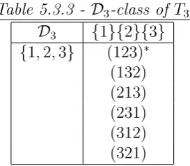
Table 5.3.3 - D3-class of T3
D3 {1}{2}{3}
{1,2,3} (123)∗ (132) (213) (231) (312) (321)
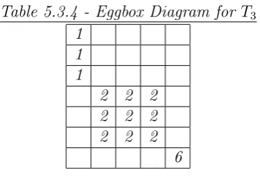
Thus, T3 has the following eggbox structure:
Table 5.3.4 - Eggbox Diagram for T3
1 1 1
2 2 2
2 2 2
2 2 2
6
We see that we get, |T3|= 6 + 9(2) + 3(1) = 27 = 33, like we should.
Each box in the D-class diagram is an H-class of T3. Each row is an
R-class of T3 and each column is anL-class ofT3. By a theorem in [4],T3 is
a regular semigroup since each R-class and each L-class contain at least one idempotent. TheH-classes ofT3 which contain an idempotent are subgroups
of T3, by a result in [4].
Using D-class diagrams, we see that we could write out the elements of T3 in terms of R-classes, L-classes, and J-classes. Since T3 is finite, the
In the next example, we will look at the D-class diagrams for Tf3. We
will see that the eggbox structure of Tf3 is quite different from the eggbox
structure of T3.
Example 5.3.3 TheD-classes of Tf3 will be described below.
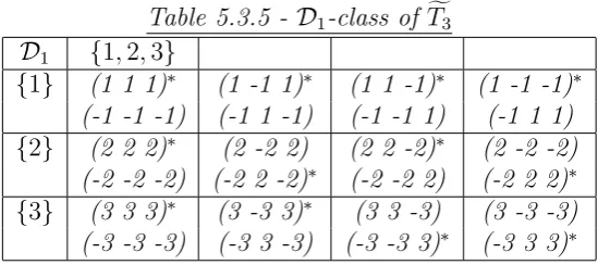
The D1-class contains the rank 1 elements.
Table 5.3.5 - D1-class of Tf3
D1 {1,2,3}
{1} (1 1 1)∗ (1 -1 1)∗ (1 1 -1)∗ (1 -1 -1)∗ (-1 -1 -1) (-1 1 -1) (-1 -1 1) (-1 1 1)
{2} (2 2 2)∗ (2 -2 2) (2 2 -2)∗ (2 -2 -2) (-2 -2 -2) (-2 2 -2)∗ (-2 -2 2) (-2 2 2)∗
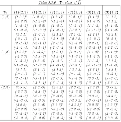
The D2-class contains the rank 2 elements.
Table 5.3.6 - D2-class of Tf3
D2 {1}{2,3} {1}{2,g 3} {2}{1,3} {2}{1,g 3} {3}{1,2} {3}{1,g 2}
{1,2} (1 2 2)∗ (1 2 -2)∗ (1 2 1)∗ (1 2 -1)∗ (1 1 2) (1 -1 2) (-1 2 2) (-1 2 -2) (-1 2 -1) (-1 -2 1) (-1 -1 2) (-1 1 2) (1 -2 -2) (1 -2 2) (1 -2 1) (1 -2 -1) (1 1 -2) (1 -1 -2) (-1 -2 -2) (-1 -2 2) (-1 -2 -1) (-1 2 1) (-1 -1 -2) (-1 1 -2) (2 1 1) (2 -1 1) (2 1 2) (2 1 -2) (2 2 1) (-2 2 1) (-2 1 1) (2 1 -1) (-2 1 -2) (-2 1 2) (-2 -2 1) (2 -2 1) (2 -1 -1) (-2 -1 1) (2 -1 2) (-2 -1 2) (2 2 -1) (2 -2 -1) (-2 -1 -1) (-2 1 -1) (-2 -1 -2) (2 -1 -2) (-2 -2 -1) (-2 2 -1)
{1,3} (1 3 3)∗ (1 -3 3)∗ (1 3 1) (1 3 -1) (1 1 3)∗ (1 -1 3)∗ (-1 3 3) (-1 3 -3) (-1 3 -1) (-1 -3 1) (-1 -1 3) (-1 1 -3) (1 -3 -3) (1 3 -3) (1 -3 1) (1 -3 -1) (1 1 -3) (-1 1 3) (-1 -3 -3) (-1 -3 3) (-1 -3 -1) (-1 3 1) (-1 -1 -3) (1 -1 -3)
(3 1 1) (3 1 -1) (3 1 3) (-3 1 3) (3 3 1) (-3 3 1) (-3 1 1) (3 -1 1) (-3 1 -3) (3 1 -3) (-3 -3 1) (3 -3 1) (3 -1 -1) (-3 -1 1) (3 -1 3) (-3 -1 3) (3 3 -1) (3 -3 -1) (-3 -1 -1) (-3 1 -1) (-3 -1 -3) (3 -1 -3) (-3 -3 -1) (-3 3 -1)
{2,3} (2 3 3) (2 3 -3) (2 3 2) (2 3 -2) (3 3 2) (3 -3 2) (-2 3 3) (-2 3 -3) (-2 3 -2) (-2 -3 2) (-3 -3 2) (-3 3 -2) (2 -3 -3) (-2 -3 3) (2 -3 2) (2 -3 -2) (3 3 -2) (-3 3 2) (-2 -3 -3) (2 -3 3) (-2 -3 -2) (-2 3 2) (-3 -3 -2) (3 -3 -2)
(3 2 2) (3 2 -2) (3 2 3)∗ (-3 2 3)∗ (2 2 3)∗ (-2 2 3)∗ (-3 2 2) (-3 2 -2) (-3 2 -3) (3 2 -3) (-2 -2 3) (2 -2 3) (3 -2 -2) (-3 -2 2) (3 -2 3) (-3 -2 3) (2 2 -3) (2 -2 -3) (-3 -2 -2) (3 -2 2) (-3 -2 -3) (3 -2 -3) (-2 -2 -3) (-2 2 -3)
In the above table, {1}{2,g 3} is the dual of {1}{2,3}.
The D3-class contains the elements of Sf3, which are all of rank 3.
Thus, Tf3 has the following eggbox structure:
Table 5.3.7 - Eggbox Diagram for Tf3
2 2 2 2
2 2 2 2
2 2 2 2
8 8 8 8 8 8
8 8 8 8 8 8
8 8 8 8 8 8
48
Each box in the D-class diagram is an H-class of Tf3. Each row is an
R-class of Tf3 and each column is anL-class ofTf3. By a theorem in [4],Tf3 is
a regular semigroup since each R-class and each L-class contain at least one idempotent.
5.4
Green’s Relations For Idempotents In
GwrT
nLet ˆe = (f, e) and ˆe0 = (f0, e0) be idempotents in GwrTn. Remember, for idempotents (f, e)∈GwrTn, e2 =e ∈Tn and f(i) = 1, for all i∈Rng(e).
We determine the R-relatedness of elements in the same manner as inTn. Recall, that ˆeisR-related to ˆe0, denoted ˆeRˆe0if and only ifRng(ˆe) = Rng(ˆe0). The number of R-classes of rank k in GwrTn is the same as the number of R-classes of rank k in Tn. So, the number of R-classes of rank k in GwrTn is n
k
!
This counting argument is proven in [3], on page 61. He uses the notation of, [4], which is the reverse of the notation found in this paper. This difference in notation is due to the fact that they write maps on the right and we write maps on the left.
Looking back to our D-class diagram for T3, we see that there are
3 1
!
= 3 R-classes of rank 1. These are the rows of the D1-class. There
are 3 2
!
= 3R-classes of rank 2. These are the rows of theD2-class. There
is 3 3
!
= 1 R-class of rank 3. This is the row of the D3-class. The same
results will hold for GwrT3. This fact will allow us to writeGwrTn in terms
of R-classes.
When describing the L-classes, the following theorem will be quite useful. The theorem works because GwrTn is unit regular, so every element is L-related to an idempotent.
Theorem 5.4.1 (Rank One Case) Ifeˆ= (f, e)is an idempotent and e0 ∈Tn
is an idempotent such that eLe0, then eLˆˆ e0 = (f0, e0), for some f0.
Proof:
Let e, e∈ Tn, where eLe0. We partition ˆn as ˆn = A1tA2 t · · · tAt. Then, for αi, α0i ∈ Ai, we have e : Ai → αi and e0 : Ai → α0i. Now, for ˆe = (f, e), f(αi) = αi. For α ∈ ˆn, if α ∈ Ai, we define f0(α) = f(α0i)
−1f(α). We must
We already know that (e0)2 =e0, so all we need to show is f0(α) = 1, for
α ∈Rng(e0). We know that Rng(e0) = α0i, so f0(α) =f(α0i)−1f(α0
i) = 1, for i = 1,2, ..., t. Therefore, ˆe0 = (f0, e0) is an idempotent. Now, we must show that ˆeLˆe0.
So, ˆeˆe0 = (f, e)(f0, e0) = ((f◦e0)f0, ee0). SinceeLe0 inT
n, ee0 =e and ((f ◦ e0)f0)(α) = (f ◦e0)(α)f0(α) = (f ◦e0)(α)(1) = f(e0(α)) = f(α), for α∈Rng(e0). So, ((f◦e0)f0, ee0) = (f, e), which implies ˆeˆe0 = ˆe.
Also, ˆe0eˆ= (f0, e0)(f, e) = ((f0◦e)f, e0e). SinceeLe0 inT
n, e0e=e0 and ((f0 ◦e)f)(β) = (f0 ◦e)(β)f(β) = (f0 ◦e)(β)(1) = f0(e(β)) = f0(β), for β ∈ Rng(e). So, ((f0 ◦e)f, e0e) = (f0, e0), which implies ˆe0ˆe = ˆe0. So, ˆeLˆe0.
Therefore, our choice of f0 was correct. 2
The above proof only covers the case of rank 1 matrices. The following example is one for which the theorem works.
Example 5.4.2 InGwrT4:
1 x2 x3 x4
0 0 0 0
0 0 0 0
0 0 0 0
L
0 0 0 0
y1 1 y3 y4
0 0 0 0
0 0 0 0
means that
x2y1 = 1 ⇒y1 =x−21
x2y3 =x3 ⇒y3 =x−21x3
x2y4 =x4 ⇒y4 =x−21x4
Both matrices used to represent the elements, 1
1 %% oo x2 2
3 x3
O
O
4 x4
^
^
=== ====
and 1 y1 //2yy 1
3 y3
@
@
4 y4
O
O
were rank one matrices. The previous theorem is also true for matrices of rank greater than one.
Theorem 5.4.3 (General Case) If eˆ= (f, e) is an idempotent and e0 ∈ Tn
is an idempotent such that eLe0, then eLˆˆ e0 = (f0, e0), for some f0.
Proof:
Once again, lete, e∈Tn, whereeLe0. We partition ˆnas ˆn=A1tA2t· · ·tAt. Then, for αi, α0i ∈Ai, we have e:Ai →αi and e0 :Ai →α0i.
Now, for ˆe = (f, e), we can write ˆe = ˆe1⊕eˆ2 ⊕ · · · ⊕et. This just saysˆ
that the matrix which represents ˆe has a block decomposition. Similarly, we may write, ˆe0 = ˆe01⊕eˆ02⊕ · · · ⊕eˆ0t.
Each block matrix in the block decomposition of ˆe and ˆe0 is of rank one. So, we are now able to relate each block of ˆe to the corresponding blocks of ˆ
e0. So, for ˆei = (fi, ei), which is an idempotent with eiLe0i in Tn, the rank one case of the theorem tells us that ˆeiLˆe0i = (f
0
i, e
0
i), for somef
0
i.
This gives us, ˆe1Lˆe01, ˆe2Lˆe02, ... ,ˆetLˆe0t. Since ˆe = ˆe1 ⊕eˆ2 ⊕ · · · ⊕eˆt and ˆ
Theorem 5.4.4 Two idempotents, eˆ= (f, e) and ˆe1 = (f1, e), are L-related
if and only if f =f1.
Proof:
Let ˆe= (f, e) and ˆe1 = (f1, e) be two idempotents which areL-related. Then,
ˆ
eˆe1 = ˆe and ˆe1eˆ= ˆe1.
This means that, (f, e)(f1, e) = ((f ◦e)f1, ee) = ((f◦e)f1, e) and
(f1, e)(f, e) = ((f1◦e)f, ee) = ((f1◦e)f, e).
So, ((f ◦e)f1, e) = (f, e) and ((f1 ◦e)f, e) = (f1, e). This tells us that,
(f◦e)f1 =f and (f1◦e)f =f1, which impliesf =f1. 2
Given e of rank k, the number of possibilities for f is |G|n−k. This is because f(i) = 1, for i ∈ Rng(e) and |Rng(e)| = k and f is arbitrary on ˆ
n−Rng(e). Hence we have the following theorem, which gives the number
of L-classes.
5.5
Looking Ahead To Chapter 6
6
Conjugacy Classes In
S
nand
T
nIn this chapter, we will examine the conjugacy classes of Sn and Tn and see many examples.
6.1
Conjugacy Classes Of
S
nRevisited
Once again, let ˆn = {1,2, ..., n}. Consider the symmetric group, Sn, which consists of the permutations of ˆn. Let α, β ∈nˆ and σ∈Sn. We say α∼β if σi(α) =β, for some i. This relation allows us to decompose into cycles.
Example 6.1.1 InS7, consider σ =
1 2 3 4 5 6 7 4 7 3 5 6 1 2
!
.
In cycle notation this element can be represented as, (1456)(27)(3). Notice that: 1∼4 sinceσ(1) = 4, 1∼5 since σ2(1) = 5,
1∼6 since σ3(1) = 6, 2∼7 since σ(2) = 7, and 3∼3 sinceσ(3) = 3.
So, we have the decomposition of nˆ = {1,2,3,4,5,6,7} into {1,4,5,6},
{2,7}, and {3}. This can be shown in graph form as follows:
1 //4
6
O
O
5
o
o
2hh ((7 3yy
We see that we have a decomposition into cycles. We may move the labels
around to produce other elements with the same cycle structure. So, we could
• //•
•
O
O
•
o
o
•hh ((• •yy
All of these elements would have the same cycle type and would be contained
in the same conjugacy class of S7.
For example,
7 //4
6
O
O
5
o
o
3hh ((2 1yy
has the same cycle structure as our original example. Thus, (4567)(32)(1)
would be in the same conjugacy class as (1456)(27)(3), in S7.
6.2
Conjugacy Classes Of
T
nNext, we will consider what happens in the full transformation semigroup,Tn. We will be able to produce a similar type of cycle decomposition. Consider the full transformation semigroup, Tn, which consists of the mappings from ˆ
n → n. Letˆ α, β ∈nˆ and σ ∈ Tn. We say α ∼β if σi(α) =σj(β), for some i, j.
Theorem 6.2.1 The relation, α ∼ β if σi(α) = σj(β), for some i, j, is an
equivalence relation.
Proof:
Reflexive: Let α ∈ n. Then,ˆ α ∼ α since σi(α) = σj(α), for i, j. This occurs when i=j. Thus, the relation is reflexive.
Symmetric: Let α, β ∈ ˆn and let α ∼β. Then, σi(α) = σj(β), for some i, j. Then σj(β) = σi(α), for some i, j, so β ∼ α. Thus, the relation is symmetric.
Transitive: Let α, β, γ ∈n. Letˆ α∼ β and β ∼γ. Then, σi(α) =σj(β), for some i, j and σk(β) =σl(γ), for somek, l.
Then, σi+k(α) = σj+k(β) = σj(σk(β)) = σj(σl(γ)) = σj+k(γ), for some i, j, k, l. Thus, α ∼γ and the relation is transitive.
So the relation is reflexive, symmetric, and transitive, which proves that
it is an equivalence relation. 2
This is the analogue of the cycle decomposition in Sn. We call this the generalized cycle decomposition. In other words, the equivalence relation yields a decomposition into connected pieces.
Example 6.2.2 InT7, consider σ=
1 2 3 4 5 6 7 2 2 1 3 7 5 7
!
.
Notice that: 1∼2 sinceσ(1) = 2 = σ(2), 1∼3 since σ(1) = 2 =σ2(3),
1∼4 since σ(1) = 2 = σ3(4), 5∼6 since σ(5) = 7 =σ2(6),
This can be shown in graph form as follows:
1
4
2
%
%
3
^
^
=== ====
5
6
o
o
7yy
Notice that we have a decomposition into generalized cycles. Relabeling
while keeping the same generalized cycle structure (or ”type”) will give us the
other elements in the same conjugacy class as our example.
So, another element in the same conjugacy class of T7 would be:
3
1
4
%
%
2
^
^
=== ====
6
7
o
o
5yy
which we could write as 1 2 3 4 5 6 7
2 3 4 4 5 5 6
!
Example 6.2.3 The following are examples of generalized cycle decomposi-tions in T10:
(1) 1 2 3 4 5 6 7 8 9 10
2 5 6 1 1 7 9 6 8 8
!
,
which we represent in graph form as,
1 //2
4
O
O
5
^
^
=== ====
3 //6 //7
10 //8
O
O
9
o
o
(2) 1 2 3 4 5 6 7 8 9 10
2 3 1 1 6 5 7 10 8 8
!
,
which we represent in graph form as,
1 //2
4
O
O
3
^
^
=== ====
5hh ((6 %%7 8oo 9
10
I
I
6.2.1 The Conjugacy Classes Of T1 and T2
The elements in each conjugacy class will be represented using one-line no-tation. An unlabeled graph will also be shown to describe the generalized cycle type of each element in the conjugacy class.
The only conjugacy class of T1 is C1 ={(1)}, which consists of elements
In T2,
The conjugacy class, C1 ={(12)}, consists of elements of the form,
•
%
%
•yy
The conjugacy class, C2 ={(21)}, consists of elements of the form,
•hh ((•
The conjugacy class, C3 ={(11),(22)}, consists of elements of the form,
• //•yy
6.2.2 The Conjugacy Classes Of T3
Again, the elements in each conjugacy class will be represented using one-line notation. An unlabeled graph will also be shown to describe the generalized cycle type of each element in the conjugacy class.
The conjugacy class, C1 ={(123)}, consists of elements of the form,
•
%
%
•yy
•
%
%
The conjugacy class, C2 ={(231),(312)}, consists of elements of the form,
•
•
o
o
•
?
?
~ ~ ~ ~ ~ ~ ~
The conjugacy class, C3 = {(132),(213),(321)}, consists of elements of the
form,
•
•yy
•
H
The conjugacy class, C4 = {(111),(222),(333)}, consists of elements of the
form,
•
%
%
•
o
o
•
O
O
The conjugacy class, C5 = {(223),(323),(121),(122),(133),(113)}, consists of elements of the form,
•
%
%
•
o
o
•
%
%
The conjugacy class, C6 = {(332),(331),(311),(232),(212),(211)}, consists
of elements of the form,
•
•
~~~~ ~~~
•
H
The conjugacy class, C7 = {(112),(131),(221),(233),(313),(322)}, consists
of elements of the form,
•
•
o
o
•
%
%
We see that T3 has seven conjugacy classes.
6.2.3 The Conjugacy Classes Of T4
Once again, the elements in each conjugacy class will be represented using one-line notation. An unlabeled graph will also be shown to describe the generalized cycle type of each element in the conjugacy class.
The conjugacy class, C1 ={(1234)}, consists of elements of the form,
•
%
%
•yy
•
%
%
The conjugacy class, C2 = {(4321),(2143),(3412)}, consists of elements of
the form,
•
•
v
v
•
6
6
•
W
W
The conjugacy class, C3 = {(1324),(4231),(1243),(1432),(2134),(3214)},
consists of elements of the form,
•
•yy
•
%
%
•
W
W
The conjugacy class, C4 = {(2413),(3142),(2341),(3421),(4123),(4312)}, consists of elements of the form,
•
•
o
o
• //•
O
The conjugacy class, C5 ={(1221),(1331),(4224),(4334),(1133),(1212),
(2244),(3434),(1144),(1414),(2233),(3232)}, consists of elements of the form,
•
@ @ @ @ @ @
@ •
~~~~ ~~~
•
%
%
•yy
The conjugacy class, C6 ={(1224),(1231),(1324),(1334),(1134),(1214),
(1232),(1233),(1244),(2234),(3234),(1434)}, consists of elements of the form,
•
@ @ @ @ @ @ @ •yy
•
%
%
•yy
The conjugacy class, C7 ={(1321),(4221),(4331),(4324),(1143),(1412), (2133),(2144),(2243),(3212),(3414),(3432)}, consists of elements of the form,
•
•
~~~~ ~~~
•
%
%
•
W
The conjugacy class, C8 ={(2112),(2442),(3113),(3443),(2121),(3311),
(4343),(4422),(2323),(4141),(3322),(4411)}, consists of elements of the form,
•
•
•hh ((•
The conjugacy class, C9 ={(2322),(4111),(4441),(3323),(2111),(2122),
(2422),(3111),(3313),(3343),(4442),(4443)}, consists of elements of the form,
•
•
• //•
W
W
The conjugacy class, C10 = {(1111),(2222),(3333),(4444)}, consists of ele-ments of the form,
• //•yy
•
?
?
~ ~ ~ ~ ~ ~ ~
•
O
The conjugacy class, C11={(1114),(1444),(2232),(3233),(1131),(1211),
(1222),(1333),(2224),(3334),(4244),(4434)}, consists of elements of the form,
•
•yy
•
%
%
•
o
o
The conjugacy class, C12={(1441),(2332),(3223),(4114),(1122),(1313),
(2211),(2424),(3344),(4242),(4433),(3131)}, consists of elements of the form,
• //•
~~~~ ~~~
•
%
%
•
O
O
The conjugacy class, C13={(1223),(1241),(1332),(1431),(2334),(4134), (4214),(3224),(1132),(1213),(1242),(1433),(2214),(2434),(3134),(3244), (1124),(1314),(1344),(1424),(2231),(3231),(4232),(4233)}, consists of ele-ments of the form,
•
@ @ @ @ @ @ @oo •
•
%
%
The conjugacy class, C14={(1322),(1323),(2324),(3324),(4241),(4211),
(4431),(4131),(1442),(1443),(2132),(3114),(2114),(3243),(2432),(3213), (1422),(2131),(4243),(3314),(2124),(4432),(3211),(4243)}, consists of ele-ments of the form,
•
•
•
%
%
•
W
W
The conjugacy class, C15={(1341),(1421),(2331),(3221),(4223),(4332),
(4314),(4124),(1123),(1312),(2241),(2344),(3431),(3424),(4133),(4212), (1142),(1413),(2213),(2414),(2433),(3132),(3144),(3242)}, consists of ele-ments of the form,
• //•
~~~~ ~~~
•
%
%
•
_
_
The conjugacy class,C16 ={(1342),(3124),(3241),(4132),(1423),(2314),(2431),(4213)},
consists of elements of the form,
• //•
•
%
%
•
_
_
@@@@@@ @
The conjugacy class, C17={(2123),(2141),(2343),(3312),(3411),(4143),
(3422),(4412),(2113),(2142),(2412),(2443),(3112),(3143),(3413),(3442), (2321),(3321),(4121),(4341),(4323),(4322),(4421),(4311)}, consists of ele-ments of the form,
•
@ @ @ @ @ @ @oo •
The conjugacy class, C18={(2311),(2421),(3121),(3341),(4122),(4313),
(4342),(4423),(2312),(2441),(3123),(3423),(3441),(4112),(4113),(2342), (2313),(2423),(2411),(3122),(3141),(3342),(4142),(4413)}, consists of ele-ments of the form,
•
•
~~~~ ~~~
• //•
_
_
@@@ @@@@
The conjugacy class, C19={(1112),(1113),(2242),(2444),(3133),(3433),
(3444),(2212),(1121),(1311),(2221),(4222),(4333),(4344),(4424),(3331), (1141),(1411),(2223),(2333),(3222),(3332),(4144),(4414)}, consists of ele-ments of the form,
•
•
•
%
%
•
o
o
6.2.4 More About The Generalized Cycle Structure
Now, we will examine the generalized cycle structure in greater detail. Let Y0 = ˆn and Yi =σi(Y0), whereσ ∈Tn. We haveY0 ⊃Y1 ⊃ · · · ⊃Yk =Yk+1.
We define, Y =Yk, to be the core of σ. We should note that σ|Y ∈SY. As we have seen in the above examples, σ produces a generalized cycle decomposition, X =X1tX2t · · · tXr, into r connected components. σi =σ|Xi is connected with core Zi =Xi∩Y. Moreover,σ|Zi is a cycle. This
means that r is the number of cycles of σ|Y.
We could represent the previous paragraphs of information pictorially. If we make a ”bullseye” diagram for the Yi’s which shows, Y0 ⊃ Y1 ⊃ · · · ⊃
Yk =Yk+1, then, the center of the ”bullseye” diagram would be Y =Yk, the core. We would use σ to divide up into connected pieces, X1,X2,X3,...,Xr,
where X=X1tX2t · · · tXr. This would illustrate the fact that σi =σ|Xi
Example 6.2.4 Consider the following element, σ ∈T9,
1oo 3
2
I
I
4
o
o oo 5
8
6 //7
^
^
=== ====
9
o
o
Using the notation described on the previous page, we see that,
Y0 = {1,2,3,4,5,6,7,8,9}, Y1 = σ(Y0) ={1,2,4,6,7,8}, and the core of σ
is Y =Y2 =σ2(Y0) = {1,2,6,7,8}. Notice that we have, Y0 ⊃Y1 ⊃Y2 =Y.
σ produces a generalized cycle decomposition, X =X1tX2, where
X1 ={1,2,3,4,5} and X2 ={6,7,8,9}.
σ1 is connected with coreZ1 =X1∩Y ={1,2} andσ2 is connected with core
Z2 =X2∩Y ={6,7,8}.
7
Conjugacy Classes in
GwrS
nConsider the wreath product of any group G with Sn, denoted GwrSn. Let Ghavet conjugacy classes, [g1],[g2], ...,[gt]. It is a well known result that we can associate a color with each cycle.
7.1
N-Cycles in
GwrS
nWe can reduce any n-cycle in GwrSn to a cycle with only one label. So, for an n-cycle,
1 g1 //2 g2
= = = = = = =
. gn
3 g3
5 g5
^
^
<<<<<< <<
4 g4
o
o
which is represented by the matrix,
0 0 0 0 · · · 0 gn g1 0 0 0 · · · 0 0
0 g2 0 0 · · · 0 0
..
. ... ... . .. ... ... ... 0 0 0 0 · · · gn−1 0
,
1 1 //2
gngn−1gn−2···g2g1
= = = = = = =
.
1
3
1
5
1
^
^
<<<<<< <<
4
1
o
o
via multiple conjugations by different matrices.
Also, by conjugation, we are able to put the gngn−1gn−2· · ·g2g1 anywhere
we wish along the n-cycle, and have all 1’s elsewhere. The conjugacy class of gngn−1gn−2· · ·g2g1 is referred to as the type of the cycle, or the color.
Example 7.1.1 InGwrS4, consider the element,
1 g1 //2 g2
4 g4
O
O
3 g3
o
o
which is represented by the matrix,
0 0 0 g4
g1 0 0 0
0 g2 0 0
0 0 g3 0