Joint state and parameter estimation to
address model error in convective scale
numerical weather prediction systems
Yvonne Muriel Ruckstuhl
Joint state and parameter estimation to
address model error in convective scale
numerical weather prediction systems
Yvonne Muriel Ruckstuhl
Dissertation
an der Fakult¨
at f¨
ur Physik
der Ludwig–Maximilians–Universit¨
at
M¨
unchen
vorgelegt von
Yvonne Muriel Ruckstuhl
aus Genf, Schweiz
Parts of this thesis are included in:
Ruckstuhl, Y. and Janjic, T.: Parameter and state estimation with ensemble Kalman filter based algorithms for convectivescale applications. Quarterly Journal of the Royal Meteorological Society. 2018; 144: 826 841. https://doi.org/10.1002/qj.3257
Janji´c, T., Ruckstuhl, Y., Toint, P. L.: An algorithm for optimization with disjoint linear constraints and its application for predicting rain. to be submitted. 2019
Zusammenfassung
Numerische Wettervorhersagemodelle ben¨otigen Anfangsbedingungen, um Wettervorher-sagen zu erstellen. Diese Anfangsbedingungen werden durch einen als Datenassimilation bezeichneten Prozess berechnet, bei dem zuvor berechnete Modellzust¨ande unter Verwen-dung neu gewonnener Beobachtungen der Atmosph¨are aktualisiert werden. Das Daten-assimilationssystem (KENDA) des Deutschen Wetterdienstes f¨ur regionale Vorhersagen basiert auf dem Ensemble Kalman Filter (EnKF), der unter der Annahme eines perfekten Modells im stochastischen Sinne und einer gaußverteilten Fehlerstatistik entworfen wurde. Da keine dieser Annahmen f¨ur operative Wettermodelle mit explizit modellierter Konvek-tion gilt, k¨onnen Verbesserungen erzielt werden indem Methoden und Algorithmen mit schw¨acheren Annahmen entwickelt werden.
In dieser Arbeit untersuchen wir die M¨oglichkeit Modellfehler zu reduzieren indem wir unsichere statistische Modellparameter unter Verwendung von Datenassimilationstech-niken st¨oren und absch¨atzen. Insbesondere verwenden wir den Augmented-State-Ansatz, bei dem Parameter durch Beobachtungen ¨uber ihre Korrelation mit beobachteten Zu-standsvariablen aktualisiert werden. Dieser Online-Ansatz bietet eine flexible und dennoch konsistente M¨oglichkeit Modellvariablen, die von den ausgew¨ahlten Parametern betroffen sind, besser an Beobachtungen anzupassen und gleichzeitig realisierbare Modellzust¨ande sicherzustellen. Eine wesentliche Herausforderung besteht darin, eine Wahrscheinlichkeits-verteilung f¨ur die Parameter zu konstruieren, welche die Unsicherheit des anvisierten Mo-dellfehlers widerspiegelt.
Wir zeigen im Rahmen eines operativen Modellsystems, dass die Darstellung von Wolken in COSMO-DE verbessert wird, wenn der Parameter f¨ur die zweidimensionale Rauhigkeits-l¨ange mit dem Ansatz des erweiterten Zustands gesch¨atzt wird. Der betrachtete Mo-dellfehler bezieht sich hier auf die Rauhigkeitsl¨ange selbst und die Oberfl¨achenfl¨usse, welche die Einleitung der Konvektion beeinflussen. Die Wahrscheinlichkeitsdichtefunktion der Rauhigkeitsl¨ange, und schlussfolgernd der Modellfehler, der den Oberfl¨achenfl¨ussen ent-spricht, wird als gaußverteilt und mit einer bestimmten Kovarianzmatrix angenommen. Die Ergebnisse sind sehr empfindlich gegen¨uber der Wahl der Kovarianzmatrix und legen nahe, wie wichtig es ist die Oberfl¨achenwindmessungen zu assimilieren.
Fehlerstatistiken annehmen zu k¨onnen. Wir zeigen in einem idealisierten Setup, dass die Sch¨atzung der Parameter durch die Einf¨uhrung von QF profitiert (auch f¨ur moderate En-semblegr¨oßen) und dass die QPEns den EnkF leistungsm¨aßig generell deutlich ¨ubertreffen. Um den hohen Rechenaufwand der QPEns zu reduzieren, schlagen wir zwei neue Ans¨atze vor. Einer der zwei vorgeschlagenen Algorithmen nutzt die Eigenschaften der zu l¨osenden Minimierungsprobleme aus, der Andere trainiert ein neuronales Netzwerk, um die durch die QPEns erzeugten Anfangsbedingungen aus den vom EnKF erzeugten Bedingungen zu reproduzieren.
Abstract
Numerical weather prediction models need initial conditions to produce weather forecasts. These initial conditions are computed through a process called data assimilation, where previously computed model states are updated using newly obtained observations of the atmosphere. The data assimilation system (KENDA) employed at the German Weather Service for regional forecasts is based on the Ensemble Kalman Filter (EnKF), which was designed under the assumption of a perfect model in a stochastic sense and Gaussian error statistics. As neither of these assumptions is valid for operational convection permitting weather prediction models, improvement can be gained by developing methods and algo-rithms for which these assumptions can be relaxed.
In this thesis we investigate the feasibility of addressing model error by perturbing and estimating uncertain static model parameters using data assimilation techniques. In particular we use the augmented state approach, where parameters are updated by ob-servations via their correlation with observed state variables. This online approach offers a flexible, yet consistent way to better fit model variables affected by the chosen param-eters to observations, while ensuring feasible model states. A key challenge is to design the probability distribution of the parameters, which should reflect the uncertainty of the targeted model error.
We show in an operational setup that the representation of clouds in COSMO-DE is improved if the two dimensional roughness length parameter is estimated with the aug-mented state approach. Here, the targeted model error is the roughness length itself and the surface fluxes, which influence the initiation of convection. The probability density function of the roughness length, and by extension the model error corresponding to the surface fluxes, is assumed Gaussian with a certain covariance matrix. The results are highly sensitive to the choice of covariance matrix, and strongly suggest the importance of assimilating surface wind measurements.
where we train a neural network to reproduce the initial conditions generated by the QPEns from those generated by the EnKF.
Contents
Zusammenfassung vii
Abstract ix
1 Introduction 1
1.1 Operational data assimilation algorithms . . . 2
1.2 General challenges for convective scale DA . . . 5
1.2.1 Observation related challenges . . . 5
1.2.2 Model related challenges . . . 6
1.2.3 Method related challenges . . . 8
1.3 Scientific Goal . . . 10
1.3.1 Approach . . . 10
1.3.2 Challenges of parameter estimation . . . 10
1.4 Outline . . . 11
2 Mathematical background of ensemble methods 13 2.1 Ensemble Kalman filters . . . 13
2.1.1 Kalman Filter . . . 13
2.1.2 Stochastic EnKF . . . 15
2.1.3 ETKF . . . 16
2.2 Localization . . . 18
2.3 Augmented state parameter estimation . . . 18
3 Evaluating data assimilation algorithms in an idealized setup 21 3.1 Data assimilation algorithms . . . 22
3.1.1 Quadratic Programming Ensemble . . . 22
3.1.2 Quadratic Filter . . . 23
3.2 Augmented state parameter estimation . . . 24
3.2.1 Localization in parameter space . . . 24
3.2.2 Dynamical model for parameters . . . 26
3.3 Experiment setup . . . 26
3.4 Results . . . 28
3.4.2 Parameter estimation . . . 31
3.5 Conclusion . . . 43
4 Estimation of roughness lengths in COSMO-KENDA 45 4.1 COSMO . . . 46
4.1.1 Parameterizations . . . 46
4.1.2 Subgrid-scale turbulence parametrization . . . 48
4.1.3 Surface Fluxes . . . 48
4.1.4 Representation of roughness length . . . 50
4.2 Observations . . . 50
4.2.1 Conventional observations . . . 50
4.2.2 Radar data . . . 51
4.2.3 Satellite data . . . 53
4.3 KENDA . . . 53
4.3.1 Localization . . . 54
4.3.2 Spread inflation techniques . . . 54
4.3.3 Observation errors . . . 55
4.3.4 Implementation notes . . . 55
4.4 Experiment setup . . . 56
4.4.1 Dynamical model for roughness length . . . 56
4.4.2 Weather situation . . . 57
4.5 Results . . . 59
4.5.1 Roughness length evolution . . . 59
4.5.2 Verification of atmospheric fields against observations . . . 64
4.6 Conclusion . . . 72
4.7 Critical look and future work . . . 78
4.7.1 Heat versus momentum flux . . . 78
4.7.2 Spurious correlations . . . 78
4.7.3 Tuning . . . 79
4.7.4 Resampling . . . 79
4.7.5 Scale separation . . . 79
4.7.6 QPEns and QF . . . 80
5 Reducing computational costs for the QPEns 81 5.1 QP for disjoint constraints . . . 81
5.1.1 Problem . . . 81
5.1.2 Background . . . 82
5.1.3 The new algorithms . . . 84
5.1.4 Performance summary . . . 90
5.2 Neural Network to replace QPEns . . . 91
5.2.1 What is a neural network? . . . 91
5.2.2 Convolutional neural network . . . 91
CONTENTS xiii
5.2.4 Experiment setup . . . 94
5.2.5 Results . . . 95
5.3 Conclusion . . . 97
6 Conclusion 101 A Verification scores 105 A.1 Bias . . . 105
A.2 Root Mean Squared Error (RMSE) . . . 105
A.3 Spread . . . 106
A.4 Fractions Skill Score (FSS) . . . 106
A.5 False Alarm Ratio (FAR) and Equitable Threat Score (ETS) . . . 106
B Proof of positive definite localized error covariance matrix 109 C KKT conditions 111 C.0.1 Equality constrained optimization . . . 111
C.0.2 Inequality constrained optimization . . . 112
List of Abbreviations 115
Bibliography 128
Chapter 1
Introduction
Throughout history, weather has strongly effected human life. From choice of clothing, to agricultural impacts, to natural disasters caused by floods and storms, even to influencing the outcome of important political wars (Ackinson, 1973). Knowing the weather ahead of time can therefore save lives and prevent severe economic losses. For millennia people have tried to predict the weather. In ancient times observation by eye was the driving mechanism. Experts would recognize recurring cloud patterns and predict their evolution based on experience. This knowledge remains valuable today, and is relied upon by many people all over the world. Nevertheless, the field of meteorology continued to develop and was brought to a new level with the invention of the electric telegraph. This facilitated the gathering of local weather reports, which were then summarized in the form of weather maps to track the evolution of atmospheric patterns, eventually leading to primitive, yet effective synoptic scale weather forecasting (Frisinger, 1978). It was not until the early 1900’s that Abbe (1901) suggested to describe atmospheric flow in terms of mathematical equations. A practical formulation of his work followed by Bjerknes (1904), in the form of an initial value problem. However, this weather prediction approach became only feasible in the second half of the century when computers began to become available. In 1922 Lewis Fry Richardson led an early attempt to manually solve the numerical equations for a six hour forecast over only two points in central Europe, but after 6 weeks of computation time, the predicted change in surface pressure was unrealistic by two orders of magnitude (Richardson, 1922). This large error was caused by an imbalance in the pressure and wind velocity fields that were used as initial conditions for the initial value problem. In contrast to humans, computers could process large amounts of data to generate proper initial conditions and subsequently provide numerical solutions to the initial value problem. This marked the beginning of numerical weather prediction (Lynch, 2008).
on simple interpolation techniques, which were superseded by more sophisticated meth-ods where a priori computed model states, referred to as the background, are used to supplement observations (Bergthorsson and D¨o¨os, 1955). A significant development for data assimilation was achieved by accounting for background and observation errors via “statistical interpolation” (Gandin, 1963), for which the foundation can be traced back to work by Kolmogorov (1941) and Wiener (1949). This method linearly combines cur-rent observations with its estimated error variance and a background state (which can be climatological or a model prediction computed from previous initial conditions) with its estimated error variance, such that the analysis is unbiased and its error variance is minimized, i.e. the analysis is the Best Linear Unbiased Estimate (BLUE) of the true state, obtained by optimizing the weights assigned to the observations and background respectively. It is important to note that statistical interpolation can be formulated as a variational least squares method (Lorenc, 1986). In others words, the problem of mini-mizing a function of weights can be reformulated to a problem of minimini-mizing a quadratic cost function of a model state. This offers a more natural framework to incorporate any dynamical constraints and solve for the analysis iteratively, which is sometimes necessary due to computational restrictions.
1.1
Operational data assimilation algorithms
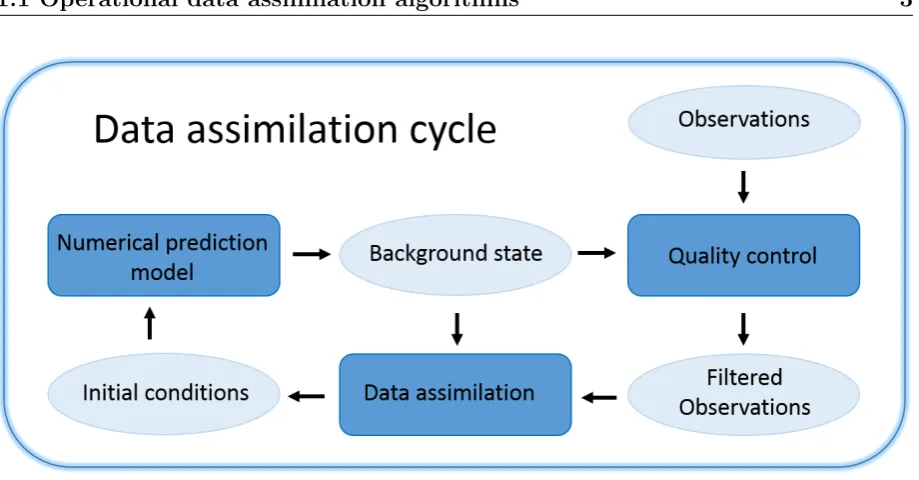
With the quality of weather prediction models and atmospheric observations available today, the background state is usually set as the most recent model forecast available at the time of assimilation, serving as a first guess of the true state of the atmosphere. This first guess is compared to available observations for quality control. Observations that are too far from the first guess are rejected to avoid physically inconsistent initial conditions as well as assimilation of poor data. The process of generating initial conditions is repeated in time to always incorporate newly available observations and is therefore referred to as the data assimilation cycle, which is schematically illustrated in Figure 1.1.1.
Data assimilation algorithms operational today are still based on least squares methods, although they differ in their representation of the error statistics as well as the implemen-tation. Which algorithm to chose depends on the resolvable scale of the numerical weather prediction model, the climatology of the region of interest, the availability of observations and their nature, and computational capacity. Perhaps the most apparent operational algorithm is 3D-Var, which minimizes a cost function J3Dvar(x), where x is a model state,
consisting of two terms: the squared distance betweenxand the background xf, weighted
by the inverse of the error covariance matrix of the background B−1, and the squared
distance between x in observation space and the observations y, weighted by the inverse of the error covariance matrix of the observations R−1
J3DV ar(x) =
1
2kx−x
fk2
B−1 +
1
2ky−Hxk
2
R−1, (1.1.1)
clima-1.1 Operational data assimilation algorithms 3
Figure 1.1.1: Schematic illustration of the data assimilation cycle.
tological information and chosen such that the analysis is well balanced. Though 3D-Var performs adequately, it has the disadvantage that it cannot handle assimilation of ob-servations at the correct time. Typically, initial conditions are computed at fixed hours, which does not necessarily match the time that observations are made. 4D-Var offers a (costly) solution by using a forward linearized model operatorMtthat propagates a model
state from initial time to time t, to compare the analysis with the observations at the correct time t = 0,1, ...T. As a consequence, the minimization is done over a trajectory
{Mtx:t= 0,1, ..., T} instead of over a single state
J4Dstrong(x) =
1
2kx−x
fk2
B−1 +
1 2
T
X
t=0
kyt−HMtxk2R−1. (1.1.2)
This formulation was referred to as strong constraint 4D-Var by Sasaki (1970), because the linearized model serves as a strong constraint for the considered trajectories. If computa-tional capacity allows it, the cost function should be relaxed to account for model error. Model error is defined as the error arising from deficiencies of the model to represent the true (projected) atmospheric state. Sources of model error are for example simplifications of model equations and their discretization in time and space. Therefore, instead of com-paring observations with a forwarded model stateMtx, they should be compared to a state xtwhich appears in an additional term of the cost function that measures the squared
dis-tance between xt and the corresponding model state Mtx, weighted by the inverse of the
covariance matrix of the error of the linearized model Q
J4Dweak(x) =
1
2kx−x
fk2
B−1 +
1 2
T
X
t=0
kyt−Hxtk2R−1 +
1 2
T
X
t=0
Figure 1.1.2: Illustrative example of sampling error and localization. The green solid line depicts the true covariance and the blue solid line the sample covariance with 40 samples. Signal to noise ratio is large when covariances are small. When covariance localization is applied, i.e. the sample covariance is multiplied by the localization function (dotted black line), the spurious correlations are damped and the result is the solid red line.
Though these variational methods are very successful, they lack non-linear flow dependent information of the background error statistics. For this reason ensemble methods like the Ensemble Kalman Filter (EnKF) (Evensen, 1994, 2003) have become important for at-mospheric data assimilation. Instead of using a fixed climatological matrix B, ensemble methods aim to compute flow dependent error statistics in the form of error covariance matrixPft from an ensemble which consists of several parallel model simulations represent-ing the probability distribution of the background field. The cost function correspondrepresent-ing to the EnKF is then
JEnKF(x) =
1
2kx−x
fk2
Pft
−1 +
1
2ky−Hxk
2
R−1. (1.1.4)
A problem that arises when applying ensemble methods, is that computational capacity only allows for a modest ensemble size, causing severe spurious correlations and rank deficiency in Pf. The solution is to use known physical properties of the model to post
process the sample error covariance matrix Pf. This process is referred to as localization.
A popular localization technique is multiplying each sample covariance Cov [xj, xl] with
0 6 c(dj,l) 6 1, where dj,l is the Euclidean distance between xj and xl, thereby reducing
1.2 General challenges for convective scale DA 5
1.1.2.
Many operational centers seek to combine ensemble methods with variational meth-ods to benefit from the advantages of both, creating hybrids like 3DEnVar and 4DEnVar (Buehner, 2005; Liu et al., 2008). The German Weather Service uses a hybrid 3DEn-Var for its global model ICOsahedral Nonhydrostatic (ICON, Z¨angl et al., 2015). Its regional model is called Consortium for Small Scale Modeling (COSMO, Baldauf et al., 2011) for which data assimilation system Kilometer-Scale Ensemble-based Data Assimila-tion (KENDA, Schraff et al., 2016) is utilized. KENDA is based on an EnKF-type method called Localized Ensemble Transform Kalman Filter (LETKF) (Hunt et al., 2007), which will be introduced in Chapter 2. In Chapter 4 we employ the COSMO-KENDA weather forecasting system and describe it there in more detail.
1.2
General challenges for convective scale DA
As mentioned before the choice of data assimilation method depends on scale, regional climate, type and availability of observations, computational capacity, but also on the goal of the weather prediction system. It is natural that the type of challenges arising from data assimilation depends on the same aspects. In this thesis we are mostly concerned with the prediction of clouds and precipitation for the mid-latitudes. We aim for practically applicable methods and are therefore constrained by the computational capacity of the German Weather Service. For a thorough overview of operational convective scale data assimilation systems and the corresponding challenges, we refer to Gustafsson et al. (2018). Most challenges for regional numerical weather prediction systems arise from the chaotic and highly nonlinear nature of convection. Unfortunately, high impact events such as thunderstorms are especially hard to forecast (Keil et al., 2014). Many studies (Lorenz, 1969; Rotunno and Snyder, 2008; Selz and Craig, 2015) indicate intrinsic limits to the predictability of both small and large scale atmospheric features. These studies also show that error growth is the fastest at small scales. Yet, with a dense observation network, a good representation of the evolution of error statistics and a method that can process all this in a statistically and dynamically consistent way, we should be able to make progress in predicting precipitation that is tied to high impact events such as storms and floods. Below we provide a brief overview of the challenges that occupy the data assimilation community.
1.2.1
Observation related challenges
possibly nonlinear, forward operator, which maps a model state to a field that allows direct comparison to the data. The development of such operators and estimating the cor-responding error variances, is not always straightforward (Zeng, 2014; Scheck et al., 2016). Moreover, the existence of correlated observation errors remains a significant challenge. Though addressed in many important studies (Weston et al., 2014; Bormann et al., 2016; Campbell et al., 2017), they are still ignored in operational weather prediction systems. In addition, the currently implemented data assimilation algorithm at the German Weather Service is constrained in the number of observations it can process. This is due to the rank deficiency of covariance matrix Pft, inherited from a limited ensemble size. Suggestions to alleviate this issue exist (Sommer and Janji´c, 2018), but have yet to be implemented and thoroughly tested.
As motivated above, a dense observational network is needed to track the evolution of convection. On the other hand, it has been hypothesized that predictability of convection can benefit from identification of synoptical forcings as well. It is however not evident how to project observational error statistics to different scales and assimilate them as such (Janji´c et al., 2018). Finally, it is not yet clear which type of observations dominate the potential quality of the model prediction. Studies have aimed to identify the relative im-portance of observations assimilated operationally (Sommer and Weissmann, 2016; Necker et al., 2018), but little can be said about the potential of observation types that have not yet been assimilated. Fabry and Sun (2010) did a study that indicates high sensitivity of the model state to vertical moisture, wind and temperature profiles, suggesting the need for dense and accurate measurements of these quantities. However, if assimilating these additional observations would actually improve a forecast cannot (yet) be verified. Further discussion of these important observation related challenges is beyond the scope of this thesis. Instead we focus on challenges discussed next.
1.2.2
Model related challenges
Naturally, the accuracy of the numerical prediction model is a key factor for the quality of the weather forecast. However, since we know that our models will never be perfect, it is important to deal with the resulting model error properly to ensure that the uncertainty of a model prediction is well interpretable. Since model errors contribute to the background error, they should be represented in the background error statistics. This is especially important for the computation of initial conditions, as overestimation of the accuracy of the background and underestimation of its covariances causes suboptimal use of observations which can lead to filter divergence (Dee, 1995).
1.2 General challenges for convective scale DA 7
model equations needs to be modeled separately in a parametrization scheme. Several successful stochastic physical parametrization schemes have been developed with the aim to account for the mean as well as the variability of the impact of unresolved processes on the mean flow (see Berner et al. (2017) for a review). However, in operational regimes these schemes are not sufficient to fully avoid under dispersion of the error covariance matrixPf. It remains therefore necessary to explicitly address model error in the data assimilation framework as well.
To complement any use of stochastic physical parametrization schemes, model error is typically accounted for by necessaryinflation techniques embedded in the data assimilation algorithm. Perhaps the simplest form is multiplicative inflation (Anderson and Anderson, 1999), where error covariance matrixPf is multiplied with a factorρ >1. Such covariance inflation techniques are helpful, but they are not designed to target specific model errors, leading to suboptimal results. As an alternative, several successful additive inflation ap-proaches have been proposed, where model error samples are added to the initial conditions in a stochastic manner. These samples can be obtained from climatological systems with the aim to account for large scale errors (Rhodin et al., 2013; Z¨angl et al., 2015), or from a higher resolution system to account for sub-grid scale scale errors (Zeng et al., 2019). Sommer and Janji´c (2018) proposed augmenting the prior ensemble with similar samples instead of adding them to the posterior ensemble, thereby creating a large synthetic en-semble at affordable cost to improve the quality of Pf. They show in an idealized setup that this method reduces the need of multiplicative inflation and localization.
scale atmospheric or ocean models. The overarching conclusion of these studies is that forecasts generally benefit from parameter estimation on short time scales, but in some cases biases are introduced on climatological scales. In addition to experiments with the assimilation of real observations, some of these studies conducted corresponding idealized experiments where different forms of model error were introduced to investigate the accu-racy of the parameter estimation under varying conditions. They all found the same as Ruiz and Pulido (2015): parameters do not converge to their true value in the presence of model error, even if they do in a perfect model setting. The effectiveness of parameter esti-mation is therefore sensitive to the application. The only explored meso-scale application that we know of was demonstrated by Hu et al. (2010), who successfully estimated two global parameters in the planetary boundary layer with the assimilation of wind profiler observations with the goal to improve the simulation of transport and dispersion of pollu-tants. We want to explore if we can improve the simulation of clouds and precipitation in operational convective-scale model COSMO by estimating one spatially varying parameter in the planetary boundary layer with the operational data assimilation system KENDA. The results are presented in Chapter 4. To the best of our knowledge there are no studies that investigate the feasibility of augmented state parameter estimation using EnKF-type algorithms in a convection permitting model with quasi-operational settings.
1.2.3
Method related challenges
The least squares approach on which all operational data assimilation methods in weather forecasting are based, only considers first and second moment statistics. Using Bayes’s the-orem, it can be shown that if all errors are unbiased and Gaussian distributed, the analysis is the most likely state, provided covariance matrices Pf and R are correct. However, at convective scales this assumption is often violated. Precipitation is an obvious example of a non-Gaussian variable. Indeed, zero precipitation often occurs, whereas negative precip-itation is absurd. As a result, the corresponding probability distribution is heavily skewed, and/or multi-modal. Ignoring this can result in poor and in some cases even unphysical initial conditions.
In contrast to the EnKF, particle filters (van Leeuwen, 2009) try to estimate full er-ror statistics, making them suitable for non-Gaussian systems. Although the benefits of particle filters have been established, the computational demands are too severe for high dimensional systems (Snyder et al., 2008). Promising efforts like implicit sampling (Chorin et al., 2010; Weir et al., 2013) and localized particle filters (Poterjoy, 2016) are made to alleviate this problem, but performance on applications such as weather forecasting has yet to be demonstrated. For this reason, EnKF-based algorithms are still a popular branch of research. Indeed, despite their sub-optimality in non-Gaussian frameworks, they have proven capable of dealing with high dimensional systems, which is vital for many practical applications. Therefore, instead of modifying particle filters to make them suitable for high dimensional systems, we are interested in strategies to modify the EnKF to deal with non-Gaussian distributions.
1.2 General challenges for convective scale DA 9
EnKF. Instead they compute a global update by simultaneously assimilating all data avail-able, thereby emphasizing the optimization of the full trajectory of the state rather than current forecasts. ES have demonstrated their worth in dealing with nonlinearity. The OSA-EnKF (Gharamti et al., 2015) and the IEnKS (Bocquet and Sakov, 2014, 2013) have shown great potential, especially for combined state and parameter estimation. However, smoothers require additional model evaluations, which is the dominating computational expense for convective scale applications. Furthermore, localization, which is necessary to deal with spurious correlations arising from undersampling, is not straight forward due to the temporal dimension included in the algorithm’s cost function (Bocquet, 2016; Desroziers, 2016).
Many modifications of the EnKF have been suggested to relax the Gaussian assump-tion. Applying transformations on non-Gaussian variables to Gaussianize the distributions (Gaussian anamorphosis) has been attempted Bertino et al. (2003), but this approach can lead to instability (Bocquet and Sakov, 2013). Static anamorphosis is more efficient on distributions that are not too dynamical (Bocquet and Sakov, 2013) which is not the case for convective scale applications. Further, state properties such as mass conservation can be lost (Janji´c et al., 2014) and transformed observation errors can lead to biased estimates (Bishop, 2016). The GIGG-EnKF (Bishop, 2016) on the other hand, directly deals with non-Gaussianity by allowing for each observed variable and corresponding observation the assumption of either a Gamma or Inverse Gamma prior distribution and/or likelihood. Results are promising for the estimation of observed state variables. However, similar to the EnKF, mapping the analysis from observation space to model space is done via simple correlations between the observed and unobserved quantities. Therefore this algorithm cannot be exploited for parameter estimation applications, since parameters are typically not represented in observation space.
1.3
Scientific Goal
We aim to investigate the feasibility of addressing model error by projecting uncertainties onto model parameters that are perturbed and estimated along with the state in a data assimilation framework.
1.3.1
Approach
We first investigate the feasibility of combined state and parameter estimation on an ide-alized test case, where we evaluate the performance of two data assimilation algorithms that were respectively designed to ensure certain dynamical properties of the initial con-ditions (QPEns) and account for skewed probability distributions of both the background and observations (QF). The model used for this study is the modified shallow water model (W¨ursch and Craig, 2014), which was designed for the purpose of testing data assimilation algorithms for convective-scale applications. In particular the model considers key proper-ties of convection that form a challenge for data assimilation: conditional instability in the form of a regime switch, and a time lag between the onset of convection and its observation. This study is meant to quantify the relative importance of conserving physical quantities and considering higher order statistical moments in the calculation of the initial conditions for convective-scale applications.
In the second part of this work, the feasibility of augmented state parameter estimation is explored in a quasi-operational setup of weather prediction system COSMO-KENDA. Specifically, we estimate the roughness length parameter z0, which is a measure of the
surface roughness that appears in the planetary boundary layer parametrization. Both the parameter itself and the parametrization of surface fluxes which are directly influenced by
z0 contain uncertainties (e.g., Rabin et al., 1990). Our goal is to project all model error
related to surface fluxes onto z0 and estimate it along with the state variables to improve
the forecast of clouds and precipitation.
The focus of the first part of this work lies on algorithmic advances (Chapter 3), whereas the second part focuses on the application (Chapter 4). Progress is made to enable inte-gration of the algorithmic related findings to the operational setup (Chapter 5), but full applicability in operational systems remains a challenge for further research.
1.3.2
Challenges of parameter estimation
1.4 Outline 11
1.3.2.1 Parameter uncertainty representation
A crucial matter is the representation of parameter uncertainty. If neither dynamics nor some form of inflation is applied to the parameters, the prediction system ebbs away the parameter perturbations, thereby prohibiting any further changes to the estimated param-eter value. It is therefore necessary to explicitly model the uncertainty of the paramparam-eters in some way. Usually solutions are integrated in the data assimilation algorithm in the form of additive noise (Gelb, 1974) or multiplicative inflation (Aksoy et al., 2006). However, it must be stressed that this choice could significantly impact the parameter evolution, since by design the feedback between static model parameters and the state is one sided, thereby gravely restricting adjustments in the structure of the error covariance matrix of the parameters. Modeling the uncertainty of static model parameters is therefore somewhat artificial in the sense that the user (partially) prescribes the error variance and covariances corresponding to the parameter. This topic is discussed further in the Chapters 3 and 4.
1.3.2.2 Localization for parameters
A complication that arises for parameter estimation is the need for localization. Localiza-tion for dynamical variables is usually based on a correlaLocaliza-tion length scale, i.e. the mean influence radius of a dynamical state element. This approach could also make sense for spatially varying parameters (such as the roughness length z0), although the parameter’s
influence radius might be hard to determine and be too small if the parameter field is non-smooth. Indeed, a spatially correlated variable has a far larger influence radius than an uncorrelated one. Determining a localization strategy for parameters is therefore not straightforward, even if they are spatially varying. For global parameters, these classic localization techniques make no sense at all, since the parameter’s influence is global by design. Aksoy et al. (2006) introduced artificial spatial structure for these parameters to circumvent the problem, but this could create biases. We therefore propose a new local-ization method for global parameters in Chapter 3. In Chapter 4 we discuss locallocal-ization for the spatially varying roughness length parameter z0.
1.4
Outline
Chapter 2
Mathematical background of
ensemble methods
Weather forecasts are based on numerical models that are designed to simulate the time evolution of an atmospheric state. To obtain a relevant weather forecast, the numerical model requiresinitial conditions that represent the current weather situation. The process of using measurements of relevant atmospheric quantities to produce these initial conditions is called data assimilation. In this thesis the focus lies on ensemble methods inspired by the Kalman Filter. In section 2.1 we introduce the Kalman Filter, the Ensemble Kalman Filter (EnKF) and the Ensemble Transform Kalman Filter (ETKF) in detail. We cover localization as way to deal with the consequences of a limited ensemble size in section 2.2 and explain how parameter are estimated with the augmented state approach in section 2.3.
2.1
Ensemble Kalman filters
The main strength of a Kalman Filter is its ability to take flow dependent uncertainties into account. Typically, a weather prediction model is imperfect due to approximations and processes that cannot be resolved on the chosen numerical grid. The measurements that are used to initialize the model contain uncertainties as well, such as instrument or representation errors. In this section we first introduce the Kalman Filter, which assumes a linear prediction model. Then we relax this assumption and describe the stochastic EnKF and the Ensemble Transform Kalman Filter (ETKF).
2.1.1
Kalman Filter
measurements y∈Rm of x. Usually m n.
xt=Mtxt−1+wt, wt∼ N(0,Qt) (2.1.1a) yt=Hxt+vt, vt∼ N(0,Rt) (2.1.1b)
where Mt ∈ Rn×n and matrix H ∈ Rm×n is a linear observation operator that maps a
state vector from model space to observation space. The subscript t = 1,2, ... indicates the discrete times at which observations are available. The goal of the Kalman Filter is to estimate the time evolution of unknown state vector x, using the model and observations described by (2.1.1).
Suppose we have an estimate xat−1 of xt−1 with error covariance matrix Pat−1 at time t−1. We use model (2.1.1a) to propagate this estimate and corresponding error covariance matrix to time t
xft =Mtxat−1 (2.1.2)
Pft =MtPat−1MTt +Qt. (2.1.3)
Model prediction xft is called the background and serves as a first guess of the true state. Note that xft and observations yt serve as two independent sources that describe the true
state vectorxt, each with known error covariance matrix. It is therefore reasonable to take
a weighted average of xft and yt to produce an updated estimate
xat =Ktyt+ (I−KtH)x f t
=xft +Kt
yt−Hxft
. (2.1.4)
Note that the corresponding error covariance matrix is
Pat = (I−KtH)P f
t (I−KtH) T
+KtRtKTt. (2.1.5)
The best linear unbiased estimate is found by minimizing the mean square error, or, equiv-alently, the trace of Pat, yielding
Kt=PftHT
HPftHT +Rt
−1
. (2.1.6)
This “optimal” Kt is called the Kalman Gain. Substituting the Kalman gain in (2.1.5)
results in a simplified expression for the analysis error covariance matrix:
Pat = (I−KtH)Pft. (2.1.7) The updated estimatexa
t ofxtis referred to as theanalysis or simply theinitial conditions.
2.1 Ensemble Kalman filters 15
Applying Bayes’s theorem to our problem yields
p(xt=x|yt, ...y0) =
p(yt|xt=x)p(xt=x|yt−1, ...y0) p(yt|yt−1, ...y0)
∝exp−1
2
(yt−Hx) T
R−t1(yt−Hx) +
x−xft T
Pft−1x−xft
,
(2.1.8)
where p(xt|yt, ...y0) is the posterior distribution, p(yt|xt) the observation likelihood and p(xt|yt−1, ...y0) the prior distribution. For simplicity we assume for now that Pft and Rt
are invertible. Maximizing posterior distribution (2.1.8) is equivalent to minimizing cost function
J(x) = 1 2
(yt−Hx) T
R−t1(yt−Hx) +
x−xft T
Pft−1x−xft
(2.1.9)
resulting in equations (2.1.4) and (2.1.6). The algorithm is summarized in Algorithm 2.1.1.
Algorithm 2.1.1 Kalman Filter
Require:
Initial state (xa
0,Pa0)
Model error statistics {Qt:t= 1,2, ...}
Observations and corresponding error statistics{(yt,Rt) :t= 1,2, ...} for t= 1,2, ... do
Prediction:
xft =Mtxat−1
Pft =MtPta−1MTt +Qt
Update:
K=PftHT HPf
tHT +Rt
−1
xa t =x
f t +K
yt−Hxft
Pa
t = (I−KH)P f t end for
2.1.2
Stochastic EnKF
The Kalman Filter was designed for relatively small linear problems. Unfortunately, weather prediction models are rarely linear. We therefore relax the linear assumption and assume
where f and h are nonlinear functions. A straightforward way to modify the Kalman Filter for (2.3.1) is using tangent linear models Mt = ∂∂xf(xt) and Ht = ∂∂hx(xt) in (2.1.3), (2.1.4) and (2.1.6). The resulting algorithm is called the extended Kalman Filter (EKF). However, as the size of the state increases, computing the error covariance matrixPft using (2.1.3) becomes infeasible. Also, linearizion of f and h might be a poor approximation as nonlinearities can be severe. To avoid direct computation of Pf and linearizion of f and h, the EnKF uses an ensemble to estimate the the background error statistics.
Let ensemble {xat−1,i : i = 1,2, ..., Nens} with corresponding ensemble mean xat−1 = 1
Nens
PNens
i=1 x
a
t−1,i consist ofNens independent samples of the posterior distribution at time
t−1. Then, at time t, {xft,i = f(xta−1,i) +wt,i : i = 1,2, ..., Nens} with ensemble mean xft = N1
ens
PNens
i=1 x
f
t,i and{yt,i =yt+vt,i :i= 1,2, ..., Nens}are independent samples of the
prior distribution and the observation likelihood respectively. From the prior ensemble, the prior sample error covariance matrix can be computed, i.e.
Pft := 1
Nens−1
XftXftT,
whereXft ∈Rn×Nens is the matrix whoseith column isxf
t,i−x f
t. However, as seen in
Algo-rithm 2.1.1, the relevant terms arePftHT and HPf
tHT. With nonlinear operator h, these
terms become N 1
ens−1X
f tY
f t T
and N 1
ens−1Y
f tY
f t T
respectively, whereYtf ∈Rn×Nens is the
ma-trix whose ith column ish(xft,i)−h(xft) withh(xft) = N1
ens
PNens
i=1 h(x
f
t,i). Ensemble {xat,i = xft,i+Kt
yt,i−h(xft,i)
:i= 1,2, ..., Nens}, whereKt=XftY f t
T
YftYftT + (Nens−1)Rt
−1
then represents the posterior distribution at time t. It should be stressed that a single en-semble member is not necessarily a meaningful estimate of the true state. Rather, the ensemble as a whole represents the statistical properties of the true state. For a meaning-ful estimate one could compute the ensemble mean, or perform adeterministic run parallel to the ensemble. This deterministic run is not perturbed during the prediction step and is updated using unperturbed observations. See Algorithm 2.1.2 for a concise description of the EnKF.
2.1.3
ETKF
A downside of the stochastic EnKF is that by representing the observation likelihood with an ensemble of perturbed observations, an additional source of sampling error is introduced. As a result, equation (2.1.7) is not satisfied exactly. The Extended Transform Kalman Filter (ETKF) avoids this, by explicitly imposing (2.1.7) on the analysis ensemble:
XatXatT = (I−KtHt)XftX f t T
(2.1.11)
whereXat ∈Rn×k is the matrix whoseith column isxa
t,i−xat. The posterior ensemble mean xa
t is computed anologous to the EnKF:
xat =xft +Kt
yt−h
xft
2.1 Ensemble Kalman filters 17
Algorithm 2.1.2 EnKF
Require:
Initial ensemblexa0,i :i= 1,2, ..., k
Initial deterministic statexa
0
Model error statistics {Qt:t= 1,2, ...}
Observations and corresponding error statistics{(yt,Rt) :t= 1,2, ...} for t= 1,2, ... do
Prediction:
xft,i =f xat−1,i+wt,i, wt,i ∼ N(0,Qt) xft =f xa
t−1
Xft =xft,1xft,2· · ·xft,N
ens
Ytf =hxft,1hxft,2· · ·hxft,N
ens
Update:
yt,i =yt+t,i, t,i ∼ N(0,Rt) K=XftYtfT YtfYftT + (Nens−1)Rt
−1
xa t,i =x
f t,i+K
yt,i−h
xft,i
xat =xft +Kyt−h
To determine the posterior ensemble perturbations we substitute ansatzXat =XftWat with
Wat ∈Rk×n into (2.1.11):
XftWatWatTXftT = (I−KtHt)XftX f t T
(2.1.13a)
=Xft
I−(k−1)−1YtfT (k−1)−1YftYftT +Rt
−1
Ytf
XftT
(2.1.13b)
=Xft (k−1)(k−1)I+YtfTR−t1Ytf
−1
XftT. (2.1.13c) leading to the following posterior ensemble perturbations
Xat = (k−1)12 Xf t
(k−1)I+YtfTR−t1Yft
−12
. (2.1.14) It can be shown that the choice of square root formulation (2.1.14) provides an unbiased posterior ensemble, in the sense that the mean of the ensemble perturbations is zero, i.e.
Xate= 0 where e is the vector with elements equal to 1 of appropriate size. The ETKF is outlined in Algorithm 2.1.3.
2.2
Localization
When the Gaussian assumption is valid andNens is large enough, the EnKF and ETKF
per-form very well. However, in practice we can often not afford an ensemble size large enough to ensure filter convergence. The solution is to use known physical properties of the model to post process the sample error covariances computed by the undersized ensemble. For example, we know that the covariance of variables at distant grid points is very small. In fact, on average, the true covariance resembles a Gaussian function of the variables’ spatial distance. This knowledge can be used to suppress severe spurious sample correlations. A natural way is to Schur multiply the sample error covariance matrix Pft with a stationary
a priori chosen localization matrixC. This technique is calledcovariance localization (see Figure 1.1.2). However, as can be seen in Algorithm 2.1.2 and Algorithm 2.1.3, it is not necessary to compute the full error covariance matrix Pft. In addition, if the observation operator is nonlinear, applying covariance localization on N 1
ens−1X
f tY
f t T
and N 1
ens−1Y
f tY
f t T
is not straightforward. A popular alternative is therefore domain localization, where one computes the analysis for each grid point separately, using only a subset of observations. The advantages of this technique are mostly computational, as the large problem is reduced to many smaller ones, which can be solved in parallel.
2.3
Augmented state parameter estimation
2.3 Augmented state parameter estimation 19
Algorithm 2.1.3 ETKF
Require:
Initial ensemblexa
0,i :i= 1,2, ..., k
Initial deterministic statexa
0
Model error statistics {Qt:t= 1,2, ...}
Observations and corresponding error statistics{(yt,Rt) :t= 1,2, ...} for t= 1,2, ... do
Prediction:
xft,i =f xa t−1,i
+wt,i, wt,i ∼ N(0,Qt) xft =f xa
t−1
Xft =xft,1xft,2· · ·xft,Nens Ytf =
h
xft,1
h
xft,2
· · ·h
xft,Nens
Update:
K=XftYtfT
YftYftT + (Nens−1)Rt
−1
xat =xft +K
yt−h
xft
Xat = (k−1)12 Xf t
(k−1)I+YftTR−t1Yft
−1 2
xa
t,i =xat +Xat(i) xa
t =x f t +K
yt−h
many state elements that are not directly observed. They can do the same for uncertain model parameters.
Let θ ∈ Rp be a model parameter that we wish to estimate, which is not represented
in observation space. Then
˜
xt:=
xt θt =
f(xt−1, θt−1) θt−1
+ ˜wt:= ˜f(˜xt−1) + ˜wt, wt∼ N
0,Q˜t
(2.3.1a)
yt=h(xt) +vt, vt∼ N (0,Rt) (2.3.1b)
where ˜x ∈ Rn+p is the augmented state and ˜Qt ∈ R(n+p)×(n+p) the corresponding model
error covariance. When provided with an initial ensemble of the augmented state and
{Q˜t : t = 1,2, ...}, Algorithm 2.1.2 or Algorithm 2.1.3 can be applied to the augmented
state, thereby yielding an online estimate of the model parameter θ as well as the model state x. The augmented error covariance matrix ˜Pft is of the form
˜
Pft := P
f
t P
f
[x,θ]t Pf[x,θ]t Pθt
!
(2.3.2)
wherePf[x,θ]t= Cov
h
xft, θft
i
andPθtis the error covariance matrix of the parameters. Note
thatPθt does not have a subscript becausePaθ(t−1) =Pfθt In this thesis we do not explicitly consider correlations between parameter errors and the remaining model error, i.e.
˜
Qt=
Qt 0
0 Qθt
(2.3.3)
where Qθt∈Rp×p will be discussed in detail in later chapters.
Chapter 3
Evaluating data assimilation
algorithms in an idealized setup
This Chapter appears in Quarterly Journal of the Royal Meteorological Society as Ruck-stuhl and Janji´c (2018). We reprint it here with some minor modifications.
We evaluate two recently developed EnKF based algorithms that either explicitly in-corporate constraints such as mass conservation and positivity of precipitation (QPEns), or introduce higher order moments (QF) on the joint state and parameter estimation prob-lem. We compare their results to the localized EnKF on a common idealized test case. The test case uses perfect model experiments with the one dimensional modified shallow water model that was designed to mimic important properties of convection. These aspects include an acute regime switch when convection is triggered (conditional instability) and a significant time lag between the onset of convection and its observation. The comparison between the QF, the QPEns and the EnKF should provide insight in the relative impact of ignoring conservation laws and physical bounds, and the skewness of relevant distributions for convective scale applications. This will aid in establishing a course for further research, i.e. either combining the algorithms or putting more effort in one direction instead. The algorithms are introduced in more detail in section 3.1
As pointed out in Aksoy et al. (2006), localization in both state and parameter space is needed when the posterior distribution is undersampled. To deal with the typically lower dimension of the parameters, the spatial updating technique was introduced. In section 3.2 we elaborate on this technique, and propose an alternative formulation to reduce computational costs. In the second part of this section we describe how we deal with severe underdispersion in parameter space, which is a common phenomenon for estimation of static parameters (see for example Simon et al., 2015).
estimate of the dynamical state for the different algorithms. Finally, a summary is provided and some conclusions and further research questions are stated in section 3.5.
3.1
Data assimilation algorithms
The data assimilation algorithms that are discussed in this chapter are modified versions of the EnKF described in Algorithm 2.1.2 (Evensen, 1994; Houtekamer and Mitchell, 1998; Evensen, 2003). With the goal to clearly indicate the respective modifications, we introduce the cost function for each ensemble member i,i= 1,2, . . . , Nens
J(δxi) :=δxTiPf
−1
δxi + [vi−Hδxi] T
R−1[vi−Hδxi] (3.1.1)
where Nens is the ensemble size. At the minimum of cost function J, δxi = xai −x f i is
the analysis increment of sizen×1 that is used to calculate analysis ensemble memberxa i
based on background ensemble member xfi (all of sizen×1). The matrix
Pf = 1
Nens−1 Nens
X
i=1
h
xfi −x¯fi hxfi −x¯fiT := 1
Nens−1 Nens
X
i=1
fi(fi)T
is the background error covariance matrix with ¯xf representing the ensemble mean, Rthe
observation error covariance matrix andHan observation operator, which for simplicity we assume is linear, of sizep×n. Theinnovation vector vi =v−i, where v=y−¯o−Hx¯f
and i =oi −¯o+H f
i is subject to perturbed observations oi, whose sample has bias ¯o.
For the EnKF, the analysis increments δxi are found by solving
min
δxi
J(δxi) for i= 1,2, ..., Nens (3.1.2)
or, equivalently,
δxi =PfHT HPfHT +R−1vi. (3.1.3) Formulations (3.1.2) and (3.1.3) of the EnKF allow us to clearly identify the differences among the algorithms discussed in this chapter. Note however that sincePf is not generally invertible, our abuse of notation in (3.1.1) strictly speaking means that a projection into the lower dimensional space would need to be done first before minimization.
3.1.1
Quadratic Programming Ensemble
3.1 Data assimilation algorithms 23
suggested in Janji´c et al. (2014), addresses this obstacle by applying physical constraints to minimization problem (3.1.2):
min
δxi
J(δxi)
subject to cj(δxi)≤0, j ∈ {1,2, ..., m1} gk(δxi) = 0, k ∈ {1,2, ..., m2}
(3.1.4)
for i = 1,2, . . . , Nens, where m1 and m2 indicate the number of inequality and equality
constraints respectively. Here, cj and gk will depend on the physical constraints that
one wishes to impose. In Janji´c et al. (2014), the effect of imposing positivity and mass constraints was investigated on simple test cases.
Since a full minimization problem has to be solved for each ensemble member, the computational cost of the QPEns heavily depends on the number and the nature of the constraints. For example, inequality constraints are algorithmically more challenging than equality constraints. Sophisticated minimization algorithms, such as interior point methods and Sequential Quadratic Programming (SQP), handle inequality constraints either by incorporating them in the cost function with a penalty term, or by solving a sequence of equality constrained subproblems instead. The non-linearity level of the constraints is an important factor as well. The higher the non-linearity, the harder the problem.
In this study we consider linear constraints only, such that problem (3.1.4) can be solved using quadratic programming (QP). For further details on QP we refer to Gill (1981), where various constrained minimization algorithms are thoroughly discussed. For the extension on QPEns to nonlinear equality constraints we refer to Zeng et al. (2017).
3.1.2
Quadratic Filter
The most restricting assumption that is needed to derive the EnKF is that all relevant distributions are Gaussian. At convective scales this assumption is typically not valid. In fact, the very nature of convection is highly non-linear and spatially irregular, which leads to skewed (and even multi-modal) distributions. The QF alleviates this issue by calculating third and fourth moments from the ensemble, in addition to the first two. The algorithm is based on an expansion which represents the analysis increment in powers of the innovation. Truncation of this expansion at the quadratic term, along with ignoring higher order terms between 3 or more variables, yields the following formulation of the QF:
δxi =
˜
PH˜T H˜P˜H˜T + ˜R
−1 ˜ vi n (3.1.5)
where ˜P =
Pf P
3
PT3 P4
, ˜R =
R R3
RT3 R4
, ˜H =
H 0
0 H
and ˜vi = [vTi ,(vv)T −(i
i)T]T, withrepresenting element-wise (Schur) multiplication. The subscriptn in (3.1.5)
dimension of δxi. The matrices P3 (R3) and P4 (R4) hold information about third and
fourth moments respectively and are obtained by ˜P= ˜ZZ˜T, where
˜
Z = √ 1
N −1
f1 . . . fN
f1 f1 −diag(Pf) . . . fN fN −diag(Pf)
and ˜ R= R T
TT F−rdrTd + 4R HPfHT
.
Hererd = diag(R), T andF are the third and fourth moment matrices of the observation
likelihood respectively. Note that for computational reasons, only higher order moments between at most two variables are taken into account. This ensures that the dimension of P3 (R3) and P4 (R4) equals that of Pf (R). In particular, P3ij (R3ij) and P4ij (R4ij)
correspond to the same variables asPfij (Rij), thereby avoiding complications with respect
to localization.
Additional computational costs with respect to the EnKF arise mainly from an aug-mented observation space. In cases where running the model forecast dominates the com-putation time, the additional costs of using the QF may be very reasonable. Also, in contrast to the QPEns, the QF is suitable for square root formulations such as the ETKF (Algorithm 2.1.3). However, like the EnKF, physical bounds are not necessarily respected (Posselt et al., 2014), as is the case for the QPEns.
A full derivation of the algorithm along with a discussion of the effect of skewed distri-butions in EnKF context can be acquired in Hodyss (2011) and Hodyss (2012).
3.2
Augmented state parameter estimation
There are two difficulties related to augmented state parameter estimation in ensemble based algorithms. Localization in parameter space θ is not straightforward since it is not obvious how to best relate global model parameter values to the analysis grid points. This complication can be circumvented using the spatial updating technique introduced by Aksoy et al. (2006). Here, we suggest an alternative to it. Secondly, augmented state data assimilation algorithms suffer from underdispersion in parameter space. Our approach to address this problem is discussed in section 3.2.2.
3.2.1
Localization in parameter space
3.2 Augmented state parameter estimation 25
Let
C=
C(x,x) CT(θ,x)
C(θ,x) C(θ,θ)
be the matrix we localize the augmented state with, where C(x,x) is a correlation matrix
of size n×n, C(θ,x) is of size 1×n and C(θ,θ) = 1 is a scalar. By Schur complement, the
matrix C is positive semidefinite if and only if C(x,x)−CT(θ,x)C(θ,x) is. If no localization
is applied to the parameters, then C(θ,x) = eT, where e is the vector with elements equal
to 1 of appropriate size. However, eTC
(x,x)e − eTeeTe < n2 −n2 = 0, and therefore
the localization matrix C is not positive semidefinite when only the state is localized. In addition, localization is typically applied to suppress spurious correlations caused by undersampling, which is an issue that should also be dealt with in parameter space.
To localize global parameters in the same way as the state, Aksoy et al. (2006) proposed to map global parameters to homogeneous fields of appropriate dimensionl (depending on the dimension one wishes to apply parameter localization to). These “dummy” fields serve to create an artificial spatial dependency of parameters, thereby allowing similar localization techniques in both state and parameter space. After the analysis increment [δxTi , δθTi ]T of size (n +l)×1 is computed, the now spatially inhomogeneous parameter
field δθi is mapped back to a scalar by performing the spatial average for each ensemble
member i. In mathematical terms, the parameter for each ensemble member is updated according to
δθi =
1
le
TC
(θe,x)Pf(θe,x)HTS−1vi, (3.2.1)
where Pf(∗,∗∗) contains the covariances between∗ and ∗∗, and
S=HC(x,x)Pf(x,x)HT +R.
Note that Pf(θe,x) of sizel×n consists of l identical rows equal to Pf(θ,x) of size 1×n and if l =n then C(θe,x) can be chosen equal to C(x,x) of size n×n.
One could argue that creating an artificial spatial dependency leads to a bias in the use of observations. Indeed, the weight that an observation is given for the parameter update is modified by a spatial dependency that does not exist. One can remedy this by using the identity matrix as correlation matrix for the parameters, C(θe,x) =I. This way, each
observation is given a relative weight that is solely determined by its error statistics and its correlation to the parameter, so that no biases of observation weights should occur. For
C(θe,x)=Ione can rewrite (3.2.1) as:
δθi =
1
nP
f
(θ,x)H
TS−1v
i, (3.2.2)
where for l = n we substituted 1leTC
(θe,x) P(fθe,x) = n1diag{Pf(θe,x)} = n1Pf(θ,x). Note
be obtained by a simple scalar parameter augmentation of the state that ensures positive definiteness of the localized error covariance matrix (see Appendix B). Global updating, where l = 1, has the additional advantage of being computationally cheaper than spatial updating, where l >1. For the EnKF this saves O(n(l−1)) operations. For the QF the reduction in computational costs is even larger. However, it is the QPEns that benefits most from the new approach, as the optimization problems are solved in model space instead of observation space.
3.2.2
Dynamical model for parameters
For any simple augmented state algorithm, the parameter spread eventually collapses due to the static nature of the parameters. For Nens → ∞ and under perfect (Gaussian)
conditions this is justified, since the only uncertainty related to parameters is the initial conditions, which should be recovered by the algorithm. However, for smaller ensemble sizes this spread collapse leads to underdispersion in parameter space.
An overview of possible approaches to circumvent this phenomenon is provided by Ruiz et al. (2013b). We choose to impose stochastic dynamics on the parameters to represent the parameter uncertainty, as for example proposed in Gelb (1974). This approach allows the user to partiallychoose the parameter distribution (and hence its uncertainty), leaving the mean to be determined by the estimation algorithm. Specifically, we set for each ensemble member i, i= 1,2, . . . , Nens
θft,i =θta−1,i+f(Xt,i) (3.2.3)
where t is the time index, f : [0,1]→
lθ−θta−1,i, uθ−θat−1,i
is a linear, bijective function andXt,i ∼Beta (αt,i, βt,i). The relation between the parametersαt,i andβt,i is chosen such
that E[f(Xt,i)] = 0. The degree of freedom that is left can for instance be used to set the
variance or shape of the distribution. Note that since the Beta distribution is bounded, the parameters cannot exceed the prescribed range [lθ, uθ] as long as the posterior ensemble
members do not exceed it. This is an advantage over using a Gaussian distribution or inflation type methods, where one would need to truncate the parameter values of the ensemble members that exceed the bounds, which affects the mean and the spread of the ensemble. An alternative would be to use a transformation of variables to guarantee that the parameters stay within their bounds, which may introduce additional nonlinearities in the parameter estimation problem.
3.3
Experiment setup
3.3 Experiment setup 27
The modified shallow water model (W¨ursch and Craig, 2014) consists of the following equations for the velocity u, rainr and water height level of the fluidh respectively:
∂u ∂t +u
∂u ∂x +
∂(φ+γ2r)
∂x =βu+Du ∂2u
∂x2, (3.3.1)
with
φ=
(
φc if h > hc
gh else, (3.3.2)
∂r ∂t +u
∂r ∂x =Dr
∂2r
∂x2 −αr−
(
δ∂u∂x, h > hr and ∂u∂x <0
0, else, (3.3.3)
∂h ∂t +
∂(uh)
∂x =Dh ∂2h
∂x2. (3.3.4)
Here, hc represents the level of free convection. When this threshold is reached the
geopo-tential φ takes on a lower, constant value φc. The parameters Du, Dr, Dh are the
corre-sponding diffusion constants, γ :=√gh0 is the gravity wave speed for absolute fluid layer h0 (h0 < hc). The small stochastic Gaussian forcingβu is added at random locations to the
velocity at every model time step, in order to trigger perturbations and hence convection. Note that this implies that the location of convection is mostly random. The parameter δ
is the production rate and α the removal rate of rain. When h reaches the rain threshold
hr (higher than hc), rain is ’produced’ by adding rain water mass to the potential, leading
to a decrease of the water level and of buoyancy. The model conserves mass, so the spatial integral overh is constant in time.
For the numerical implementation of the model, the one dimensional domain, represent-ing 125 km is discretized with 250 points, yieldrepresent-ing the state vector x= [uThTrT]T ∈
R750.
The time variable is discretized into time steps of 5 seconds. The Gaussian stochastic forcing βu has a half width of 4 grid points and an amplitude of 0.002 m/s. The
param-eters that are estimated along with the dynamical state are α ∈ [lα, uα], φc ∈ [lφc, uφc]
and hr ∈ [lhr, uhr] (see Table 5.1.1 for values of upper and lower bounds). As previously
stated, the multiplicative parameter α regulates how fast rain decays. Parameter hr is
responsible for a possible switch between the regimes, since it determines when it starts to rain. Parameter φc is a value of geopotential once the level of free convection is reached
and influences the total time required for a cloud to develop to full height. Each ensemble
Parameter Lowerbound
l
Upperbound
u
α 0.0003 0.001
φc 899.7 899.9
hr 90.15 90.25
Table 3.3.1: Lower and upper bounds for the parameters to be estimated.
values drawn randomly from the uniform distributionsU(lα, uα),U(lφc, uφc) andU(lhr, uhr)
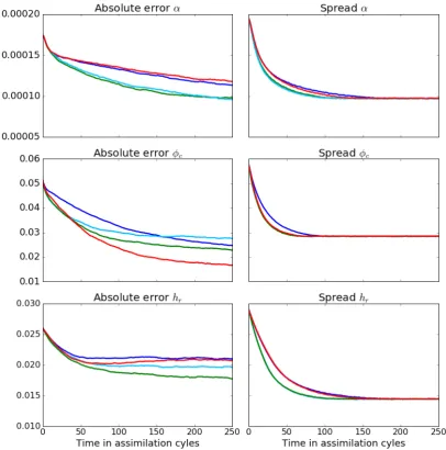
respectively. After an appropriate spin up time, 250 assimilation cycles are performed. All experiments discussed below need about 50 cycles to converge to a constant mean RMSE value. Therefore, the average of the RMSE over the last 100 cycles is computed to assign a scalar RMSE value to each experiment. For statistical significance, the final score used in the results is the average RMSE over 250 experiments.
Unless stated otherwise, observations are taken from the nature run every 60 model time steps (equivalent to 5 minutes in real time). A Gaussian observation error is added to the wind uand height h fields with a standard deviation of σu = 0.001 m/s and σh = 0.02
m, and a lognormal error is added to the rainr field with parametersµ=−8 and σ = 1.8, yielding a very small observation bias of 0.000825 and standard deviation of 0.00185. For all variables the observation error is roughly 10% of the maximum deviation from the variable mean. To mimic radar data, observations for all variables are available only on grid points where rain above a threshold of 0.005 dBZ is measured. Therefore, the rain data has a known observation bias of 0.000825 dBZ wherer >0.005 dBZ in the nature run. Note that with a probability of 6.7%, observations corresponding to a dry grid point in the nature run are also assimilated. For rain, these observations have a bias larger than 0.005 dBZ. A random selection, amounting to 25% of the remaining grid points, of additional wind observations are assimilated, which represents additional data available (for example obtained from aircraft).
To deal with undersampling, covariance localization according to Gaspari and Cohn (1999) is applied with a fixed localization radius of 6 grid points for all three algorithms. This corresponds to the localization radius for which the EnKF yields minimum analysis RMSE values of the rain variable for small ensemble sizes. For the spatial updating tech-nique described by (3.2.1), the localization matrix for the parameters is the same as for the state. For global updating we use Ccov(θ,x) = 1neT as discussed in section 3.2.1. For
the dynamical model of the parameters according to (3.2.3) we choose to use the second degree of freedom to set a lower limit on the parameter spread. This limit is set to 25% of the initial spread. An interior point method is used to solve the quadratic minimiza-tion problems of the QPEns. The constraints that are applied are mass conservaminimiza-tion, i.e.
eT(ha−hf) = eTδh= 0, and positivity of precipitation, i.e. ra =δr+rf ≥0. For the QF and the EnKF negative values for rain are set to zero if they occur.