THE DISTRIBUTION OF MUTANT ALLELES IN A SUBDIVIDED POPULATION

(1)

THE DISTRIBUTION

OF

MUTANT ALLELES I N A SUBDIVIDED POPULATION

MONTGOMERY SLATKIN

Department of Zoology, NJ-15, University of Washington, Seattle, Washington 98195

Manuscript received September 14, 1979 Revised copy received February 19, 1980

ABSTRACT

The results are presented from a simulation study of the spatial distribution of mutant alleles in a subdivided population. Statistical measures of the spatial pattern are defined in such a way that the same quantities could be measured in a geographic survey of allele frequencies in natural populations. Two types of quantities are discussed in this paper: (I) the occupancy distribution

provides information on the presence or absence of the mutant in different numbers of demes; and (2) the conditional frequency distribution provides information about the extent of local differentiation when the mutant is present in different numbers of demes. Properties of these distributions are found for different types of natural selection acting on the mutant. Some results are presented for the same statistical measures based on samples of individuals from a fraction of the total number of demes. The simulation results for intermediate levels of the migration rates are compared with analytic results obtained on the limits of high and low migration rates. The main conclusion is that these measures of the spatial distribution of mutants in a subdivided population have simple properties that could provide a new perspective on data from natural populations.

T H E

spatial distribution of alleles in a subdivided population may reveal some aspects of the breeding structure of the population and some indication of the selection acting on those alleles. CAVALLI-SFORZA ( 1966) has emphasized that, even when the breeding structure - the migration rates and effective local population sizes

-

is unknown, the breeding structure must be the same for all alleles and loci. Using this fact, LEWONTIN and KRAKAUER (1973) attempted to look for consistency of allele distributions to determine whether selective neutrality could, under any breeding structure, account for the observed distributions. While there were statistical defects with their analysis that weaken their conclusions (NEI and

MARUYAMA

1975; ROBERTSON 1975), their basic approach remains valid. To use that approach, however, new theoretical results are needed that provide useful measures of allele distributions in subdivided populations. In this paper, I will show that there are some simple properties of the spatial distribution of mutant alleles in subdivided populations. In another paper (SLATKIN, in preparation)

,

I will discuss the application of these results to data.

(2)

504 M. SLATKIN

One approach to the analysis of subdivided population is to look for those properties that do not depend on the breeding structure of a population.

MARUYAMA

(1970, 1971,1972,1974) showed that, for a n allele with no domiance, the proba-

bility of fixation, the net heterozygosity and the conditional heterozygosity do not depend on the pattern of spatial subdivision, only on the selection coefficient and total population size. Lack of dependence of fixation probabilities on population structure can also be derived from the branching process formulation of POLLAK

(1 966), although he did not obtain that result.

NAGYLAKI

(1 977) showed that, in

many cases, the rate of loss of heterozygosity in the absence of selection depends only on the population size and not on the pattern of spatial subdivision.

An alternative approach to the study of subdivided populations is to take population structure explicitly into account and to find those features of a genetical model that depend on the actual pattern of spatial subdivision. WRIGHT,

DOB-

ZHANSKY and

HOVANITZ

(1 942) estimated the dispersal distance of Drosophila

pseudoobscura from the frequencies of allelism of recessive lethals found at different distances. CRUMP and GILLESPIE (1976, 1977) and SAWYER and

FLEISHMAN

(1979) found the distribution of dispersal distances of new mutants, using tech-

niques from the theory of branching diffusion processes.

This paper extends the results of SLATKIN and CHARLESWORTH (1978), and the approach is that of the second group of papers, in particular that of

WRIGHT,

DOBZHANSKY

and

HOVANITZ

(1 942). Using a simulation program to model the progress of a mutant allele in a subdivided population, the properties of some measurable quantities are found. We will see that, despite the complexity of the underlying model, these quantities have surprisingly simple properties.

THE SIMULATION MODEL

All of the results presented below were obtained using a computer simulation program that models the combined effect of genetic drift, selection and gene flow

on a diallelic locus in a diploid species. The program is similar to that used by SLATKIN and CHARLESWORTH (1978), but is modified to be more efficient and to obtain new derived statistics. Following the terminology of SLATKIN and CHARLES-

WORTH (1978), a population is assumed to consist of n demes, numbered 1 through

(3)

MUTANT ALLELE DISTKiBUTION 505

All of the simulations are started with only one copy of

A,

the mutant allele.

If

s2 2 s1

>

0, then the mutant is advantageous; if s2 5 s1

<

0, it is deleterious.

The gene-flow stage is the only one in which the geographic arrangement of the demes enters. All of the information about the geography is contained in a list of demes with which each deme exchanges alleles and the rates of exchange with each. This approach was also used by

BOORMAN

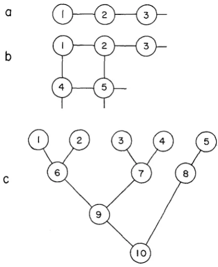
(1974). Some examples are shown in Figure 1, where three of the gene-flow patterns analyzed are illustrated. Figures l a and l b show the one- and two-dimensional stepping-stone model of

KIMURA (1953). This device for representing a stepping-stone model of a sub-

divided population allows the direct analysis of a more complex geographic pattern without any modification of the program. Figure I C could represent a population found in a river system. I t is modelled by linking demes 1 and

2

to 6, deme 7 to demes 3 , 4 and 9,etc.

In the simulations discussed

in

this paper, only one type of gene flow pattern was used. The same fraction, m, of the gamete pool in each deme is replaced each generation by gametes derived from demes that are linked to it. Equal weight is given to all demes linked to a given deme. For example, in the linear stepping-

a

C

FIGURE 1.-Three examples of the geographic arrangements of demes used in the simulation program. A link between 2 demes indicates that gene flow occurs between those demes. (a) A

linear stepping-stone model (n

x

1 array). (b) A two-dimensional stepping-stone model (nlz n2 with n = nl-n2). (c) A more general stepping-stone model representing a riverine system with

(4)

506 M. SLATKIN

stone model, all demes except the two demes at the ends receive m/2 of their gametes each generation from each of the two adjacent demes. Deme 1, however, receives a fraction m from deme 2. Thus, the migration pattern is not completely symmetric because deme 1 contributes less to deme 2 than the reverse. Clearly, for each geographic structure, there is an equivalent symmetric model, but the few such cases that were run showed no detectable differences in the overall pattern in the results. Which model is more realistic depends on the dispersal pattern of the particular species being considered.

This model of gene flow differs from that used by SLATKIN and CHARLESWORTH

(1978). In that paper, adults instead of gametes were assumed to move. Analytic

theory (SVED and LATTER 1977) shows that the differences between the two types of gene flow are of the order of m/N and not likely to affect the results for the range of parameter values used in this simulation. With deterministic gene flow at the gamete stage, only one sampling step each generation is necessary instead of two, making the program more efficient.

The process of random mating is modelled by generating 2N random numbers uniformly distributed in (0,l) and counting the number greater and less than the frequency of A as modified by selection and gene flow. That implies that the effective deme size is the same as the actual size, N . The random number generator (RAN) supplied with the DEC RT-I1 (Version 3 ) FORTRAN operating system was extensively tested by using analytic results.

To summarize, the following parameters had to be specified for each simulation: (1) n, the number of demes; (2) the list of demes from which each deme draws gametes during the gene-flow stage and which defines the geographic arrangements of demes; ( 3 ) m, the fraction of gametes in each deme drawn from other demes; (4) s1 and sz, the selection coefficients on the Aa and aa genotypes, assuming A A has a fitness of unity;

( 5 )

N , the actual and effective size of each deme.

All of the simulations were run in the same way. For each case with a given set of parameter values, a predetermined number of replicates was run. Each replicate was initiated by setting p ( j ) to zero in all demes except one, in which it was set to 1/2N, indicating that a single A allele is in one of the demes. The initial deme was chosen randomly for each replicate to model the random occurrence of mutations. Each replicate was then continued until the mutant was either lost or fixed, at which time another replicate was started.

(5)

MUTANT ALLELE DISTRIBUTION

507

For the sampling process there are three additional parameters that must be specified for each set of replicates: the number of demes sampled, nsum, the number of individuals sampled from each deme, N,,,, and the interval between successive samples, set at 50 generations for all results presented later. When a sample was taken and nsum

<

n, the nsm demes were chosen at random.

RESULTS

Data obtained by sampling allele frequencies in a subdivided population or from these simulations can be viewed in at least three different ways. The first is to consider only the presence or absence of alleles in each deme. The second is to consider the distribution of frequencies of an allele only in those demes in which that allele is found. The third is to consider the relationship between the spatial distribution of allele frequencies and the migration pattern among the demes. In this paper, the results from the simulations that are relevant for the first two ways will be presented. The results relevant for the third way will be described in a later paper.

The information about the presence or absence of the mutant in the different demes is contained in the probability distribution of the number of demes in which the mutant is present, given that it is neither fixed nor lost in the population. This distribution was introduced by SLATKIN and CHARLESWORTH (1978) and denoted by Pi where i takes values from 1 to n and

n

B P ; = 1 .

The distribution, P i , will be called the occupancy distribution and

i

the occupancy number of the mutant at a particular time. The occupancy distribution can be estimated from the simulations by accumulating over all replicates the number of generations in which the occupancy number takes on different values and then dividing at the end of the set of replicates by the total number of generations. In SLATKIN and CHARLESWORTH (1978)

,

the distinction was made between the occupancy distribution for alleles that are ultimately fixed and those that are ultimately lost. While there are some interesting comparisons between these conditional occupancy distributions for alleles with different selection coefficients, it is impossible to determine in a particular sample of allele frequencies which alleles would become fixed or lost. Thus, that distinction is not useful for considering data and will not be made here.

The main result is that the occupancy distribution can be described by a discrete distribution derived from a beta distribution. For a continuous random variable, x, defined on the interval ( O , l ) , the beta distribution has the form

i=1

f(z) = CZa-'(l--z)b-l

(6)

508 M. SLATKIN

For a given P+ generated by a set of replicates with particular parameter values, the parameters a and b can be determined by comparing mean and variance of

Pi

with those of f(x). If

and

then f(z) will have meanT/n and variance V / n 2 when

-

a = i 2 ( 1 -Tin) /V-i7/n

and

b

=a(n/F-l)

(JOHNSON and KOTZ 1970, p. 44). The matching of moments with the continuous rather than the discrete distribution is done because there is an analytic formula for the continuous distribution.

A

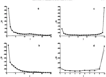
numerical study of random numbers generated by a beta distribution showed that the bias introduced by this method is small when n is 10 o r larger.

There are two different shapes for the occupancy distribution generated by the simulations. For advantageous or neutral alleles, a U-shaped distribution was found for which the computed values of a and b were both less than one, as shown

in

Figure 2c. For a deleterious mutant, a J-shaped distribution was found for which a was generally less than 1 and b greater than 1, as shown in Figure 2a and 2b. In some cases the computed values of a and b were both greater than one, with the value of b being much larger than a. In such cases,

f(z)

is unimodal, but with the mode falling in the interval, (O,l/n) generating J-shaped fi.

(7)

M U T A N T ALLELE DISTRIBUTION 509

.3m

Pi

I

.lW

7 h

i

.uD*

b

.uD

'7

C

p"

i

d m

i i

FIGURE 2.-Four examples of the fit of a beta distribution to the occupancy distribution, Pi.

The symbols connected by a solid line indicate the values of P, obtained from the simulations, and the dashed line indicates the values of the beta distribution fit by matching the fist and second moments. In all cases, the results are based 011 1000 replicates for a 5

x

5 array of demes with N = 100, s2

=

2s1 = 2s. Figures 2a, b and c are based on complete information, and Figwe 2d is based on samples of size 25 taken from 10 randomly chosen demes. (a) s=-0.001;

m = 0.05. (b) s = -0.001; m = 0.01. (c) and (d) s = 4-0.002; m = 0.01.

TABLE 1

Values of the standard x 2 statistic measuring the goodness of fit of the Pi to a beta distribution

S a b Sample size df

-

m

0.005 -0.002 0.89 7 . 4 171 2 2.69

0 0.26 0.28 378 6

**a*

S0.002 0.33 0.35 338 8 38.7*

m=0.05 -0.002 0.72 2.46 178 8 12.4

0 0.41 0.26 44.2 8 34.1 *

4-0.002 0.35 0.22 419 8 70.1*

(8)

510 M. SLATRIN

from the fitted beta distribution. On the other hand, all the cases with a U-shaped occupancy distribution deviate significantly from the fitted distribution.

There are two possible explanations for the significant deviations. One is that the Pi actually fit the f z but that the samples taken every 50 generations are still not sufficiently independent in the cases that produce a U-shaped distribution for the actual sample size to be appropriate far the statistical test. The U-shaped distribution is generated by alleles going to fixation, a process that takes a long time -on the order of hundreds w thousands of generations for these parameter values. That could cause a significant correlation between samples taken even 50 generations apart. For the J-shaped distributions generated by alleles that are ultimately lost, with a mean time to loss on the order of 10 to 20 generations f o r these parameter values, successive samples were usually taken from different replicates ~

The other explanation is that the U-shaped occupancy distributions do not fit the f z , but are merely close. From careful examination of the simulation results, there were found small but consistent deviations from the beta distriibution, with the fitted values being slightly larger for the intermediate occupancy numbers. One example is shown in Figure 2d, which is typical of the cases in which deviations, from the beta distributions were found. These deviations do not invalidate the use of the parameters of the beta distribution as a description of the OCCU- pancy distribution, since the character of the occupancy distribution is well matched by the beta distribution in all cases. However, it does mean that a n analytic treatment of this problem would not be expected to yield a beta distribution as the true occupancy distribution.

For a given set of demes and pattern of migration, the values of a and b depend on the intensity of selection ( s l and s,) and migration rate ( m ) . The effect of increasing m is to decrease the values of a and b and to decrease the ratio b/a. Some examples are shown in Table 2. For a U-shaped distribution, a decrease in a and b

has the effect of pushing the distribution more against the two axes. For a J-shaped distribution in which b

>

1, a decrease in a and b with a decrease in the ratio b/a

(9)

MUTANT ALLELE DISTRIBUTION

511

Considering the effect of different intensities of selection on the mutant, stronger selection acting on a deleterious mutant has the effect of increasing both

a and b and the ratio bJa (Table 2 ) . Stronger negative selection on the mutant pushed the

Pi

distribution against the axis. This effect is also shown in Table 1 of SLATKIN and CHARLESWORTH (1978). Note that, although the selection on the mutant in each deme could be regarded as weak ( I N S / = 0.1,0.2,) the changes of the values of a and b are relatively large. For an advantageous mutant, an increase in the selection intensity has the same effect as an increase in the migration rate. The intuitive explanation is the same as for the effect of changes in the migration rate. Stronger selection makes an advantageous mutant sweep through the intermediate occupancy numbers more quickly than a mutant that is less strongly selected.

Differing degrees of dominance make little qualitative or quantitative difference in the form of Pi. In all cases simulated, the fit to the f i distribution was as good as in the cases with no dominance.

The effect of changes in the size of the demes is simple and could be anticipated. The values of a and b were found to depend only on the products Nm, Nsl and

Ns,.

The effect of changes in the migration pattern are similar to changes in the migration rate. As discussed in SLATKIN and CHARLESWORTH (1978), the most important difference is between a one-dimensional stepping-stone model and geographic arrangements that allow more migration, such as a two-dimensional stepping-stone model. As shown in Table 3, the difference between the results for a one-dimensional stepping-stone model and the three others is less than the differences among the others.

If

samples of individuals are taken from some of the demes, the results depend most strongly on the number of demes sampled. If all of the demes are sampled, but only some fraction of the total number of individuals is taken, the computed values of the parameters a and b are nearly the same as i f all the individuals in each deme were sampled.

For

example, for a

5

x 2 array of demes of size 100, values of a = 0.58 and b = 0.53 were obtained for a neutral mutant, assuming all individuals in each deme were sampled and values of a = 0.53 and b = 0.51 if only 25 individuals per deme were sampled. In all cases, the values of a and b for the samples of size 25 are smaller by a few percent than those values from complete

TABLE 2

Values of the two parameters of a beta distribution fitted to P, for different parameter values

I. 5

x

5 array of demes (n=25).

m 0.005 0.01 0.05

S a b ta b a b

-0.002 0.68 9.53 0.4Q 2.61 0.50 2.14

0 0.15 0.23 0.171 0.281 0.37 0.18

+0.002 0.18 0.29 0.41 0.19 0.16 0.08

In all cases, s2 = 2s, = 2s, and there were lo00 replicates.

(10)

5

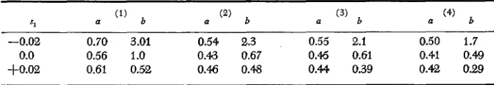
12 M. SLATKIN

TABLE 3

Comparison of values of a and b for beta distribution fitted to Pi

(3)

a (4)

-0.02 0.70 3.01 0.54 2.3 0.55 2.1 0.50 1.7

0.0 0.56 1.0 0.4 0.67 0.45 0.61 0.41 0.49

+OD2 0.61 0.52 0.46 0.48 0.M 0.39 0.42 0.29

In all cases, n=10, m=O.l, s2=2.s, and 5000 replicates were run for each set of parameters. The geometric arrangements of demes were: (1) 10

x

1, linear; (2) branching pattern shown

in Figure IC; (3) 5

x

2, rectangular; (4) Island model.

samples

( N

= 100). However, when fewer than the total number of demes are sampled, there is a large difference between values of a and b from the samples and from complete information, For a 5 X

5

array of demes of size 100 with m = 0.0,1, the values of a = 0.17 and b = 0.28 were obtained from complete information, while values of a =0.29 and b = 0.33 were obtained from samples of 25 individuals from 10 randomly chosen demes. The values of a and b estimated from samples are larger than those based on complete information, although the change in the value of b is small when the Pi distribution is J-shaped.

There is another way to consider the occupancy distribution based on samples, one that is more relevant to the application of these results to data. We can assume that the actual number of demes, n, is unknown o r not known with any precision. We can consider a samples of size N,,, from a given number, nsam, of demes and ask how the computed values of a and b depend on the actual number of demes. With this approach, the values of a and b based on complete information are un- important. A set of results for samples of the same size and from the same number of demes is shown in Table

4

for three different values of n with comparable geometric arrangements of demes. Qualitatively, the results do not depend on n, but

the computed values of a and b differ, though not in a consistent or obvious way. The second type of information generated by the simulations is on the distribution of mutant frequencies in those demes that contain the mutant. For a mutant with occupancy number

i,

we could define the joint distribution of the

i

nonzero frequencies. There would be one such distribution for each value of

i.

Too many replicates would be required to estimate these joint distributions, so that only cer-

TABLE 4

Comparison of va2ues of a and b for a beta distribution fitted to the occupancy distribution based on samples taken from randomly chosen demes

5 x 5 (n=!25) 4 X 4 (n=16) 5 x 2 (n=10)

S a b a b a b

-0.002 0.5M 2.58 0.588 2.71 0.642 3.47

0 0.292 0.332 0.325 0.415 0.535 0.514

+0.002 0.666 0.261 0.472 0.547 0.387 0.398

(11)

MUTANT ALLELE DISTRIBUTION 513

tain statistics of them will be discussed.

For

each i, the average frequency in the occupied demes, j j

(i)

; the maximum frequency, pm

(i)

; and the standardized variance, FBT

(i)

= u*/p (1

- p )

can be defined. They can be estimated by accumulating the appropriate values in each generation and then dividing at the end of a set of replicates by the total number of generations spent in each occupancy number.

The main result from the simulations is that all of these statistics, which are functions of

i, are only slightly dependent on the selection coefficient acting on the

mutant. It appears from the simulations that, for relatively weak selection in each deme ( N s , and N s , less than 0.5 in absolute value), the differences between these functions of

i

are of the same order of magnitude as

1/N.

Thus, for even moder- ate large demes

( N

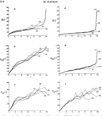
= 2 5 ) , these functions are independent of s for all practical purposes. While this range of selection coefficients could be regarded as modeling weak selection in each deme, the gene flow between the demes can make the effective size of the population much greater than the local deme size. It is worth recalling that there were large differences in the occupancy distributions generated by the different selection coefficients in this range.

We can see the character of the statistics, ji(i), pmw((i) and FST

(i)

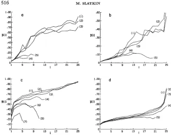
in Figure 3. In the left hand set of graphs (Figures 3a, 3b and 3c), the results are shown for five different selection schemes, all with no dominance, for one migration rate, m=0.01. The set of graphs on the right shows the results for the same selection coefficients, but for a higher migration rate, m=0.05. There are several features

of the graphs that are typical of the results obtained for other parameter values. First, the differences between the curves for different selection coefficients are somewhat larger for the lower migration rate. Second, the curves for the higher migration rate are smoother and less variable in their shape than for the lower migration rate. Each curve was generated by averaging over 1000 replicates, and it was found that there was more variability in the results for smaller migration rates. Third, there is a large difference between the sets of curve for the different migration rates, with the lower migration rates having consistently higher values of the statistics for the same occupancy number. (Note the differences in the verti- cal scale.) Thus, while there is only weak dependence on the selection coefficients, there is strong dependence on the migration rate.

There does not seem to be a simple analytic function that fits any of these curves for a large range of parameter values and geometric arrangement of demes. In some cases, an adequate description of

p

(i) or pmm

(i) can be obtained by fitting a

linear function (c

+di)

or a log-linear function [c

+

d.log(i) ] for small values of

(12)

514 M. SLATKIN

.70-

.80

.70 .60

.SO s o

.50

F(i) .,o D(i) . 4 0 -

3 0

.20

.XI

.20

.IO .lo-

( 1 )

d

- (2)

-

- (3)

-

(41

'

1 5 9 13 , 17 21 25

I

.IO-

.08 FsT(i) .06

.04

.02 (41

I

-

.40

.30

.20

.10

(4)

f

I / >

'1 5 9 13 17 21 25

FIGURE d.-Graphs of three statistics, p(i), p , , ( i ) and FST(i), of the mutant frequency distributions conditioned on the occupancy number i. In these graphs and throughout, these statistics are defined only a t integer values of i, and the values at those points are connected by solid lines. These curves are based on complete information from the simulatioas of 5

x

5 arrays of demes with N = 100 and sz = 2s, = 2s. In all graphs, the curve numbers associated with different values of s are: (1) s = 0.002; (2) s = 0.001; (3) s = 0; (4) s = -0.001; ( 5 ) s =

-0..002. For (a), (b) and (c), m = 0.01; for (d), (e) and (f) m = 0.05.

(13)

dependence on

i

and the parameters, the results for only one, j j ( i ) , will be presented.

There are several different modifications that must be considered in order to understand the implications of these results. The effects of the geometry of the population can be anticipated from the results for the occupancy distribution. For a more restrictive geometry, such as a one-dimensional stepping-stone model, but with the same migration rate, the results are comparable to those from a two- dimensional stepping-stone model with a lower migration rate. This is illustrated in Figures 4a and 4b. These two graphs show another characteristic of the results for lower migration rates. The more strongly selected, deleterious mutants gen- erate p ( i ) curves that differ from those generated by neutral and advantageous mutants. Typically, when the curves for the more deleterious mutants are different, they lie below them, indicating smaller average frequencies for each OCCU- pancy number, and they terminate at some occupancy number less than the maximum, n, the total number of demes. Also, they are often unimodal rather than monotonic. In such cases, the actual maximum occupancy number reached

in

different sets of the same number of replicates and the same parameter values is unpredictable, but the resulting occupancy distribution in such cases is zero, or effectively so, for intermediate and large occupancy numbers.

For populations with the same geometric arrangement of demes, there is a slight difference between the results for cases with different deme sizes ( N ) , but with the same values of the products, Nm, Ns, and Ns,. Two examples are shown in Figures 4c and 4d, which correspond to Figures 3a and 3d. The curves in Fig- ures 4c and 4d are smoother than those in Figures 3a and 3b because more replicates (5000) could be run for each case. Both the range of variation of the curves and their general shape are the same, but the set of curves for N=10 is shifted up- ward by approximately 0.08. Also the curves for N=100 increase slightly more rapidly than do those for N=10. However, in this and other cases, the general characteristics of the curves depend only on the products, Nm, Ns, and N s 2 .

TABLE 5

Values of the parameters of a least-squares fit of the curve c

+

d . i to p(i)

~~~~ ~ ~~

m S C d i m S C d i

0.005 (-0.002 0.037 0.089 5 0.05 ,-0.002 0.013 0.012 12

+0.002 0.038 0.080 7 +0.002 0.012 0.011 11

0 0.044 0.066 9 0 0.013 0.014 10

of

0.0% 0.047 11 0 0.011 0.014 I2 0.01 - 0 . W 0.025 0.037 15 m=0.05* -0.002 0.012 0.013 15

+o.m

0.021 0.060 l e +0.00.2 0.012 0.011 9

* Second set of cases with same parameter values.

+

5000 replicates.

(14)

516 M . SLATKIN

(21 .En

.70 (31

.60

.50

.40

.30

2 0

.IO

F(i)

'1 5 9 13 17 21 25

I

I I

'1 5 9 13 17 21 25 '1 5 9 13 17 21 25

FIGURE 4.-Values of p ( i ) based on complete information for different parameter values. In all cases, s2 = 2s, = 2s. Figure (a) and (b) are from simulations of 25

x

1 arrays of demes

with N = 100. In (a) and (b), the curve numbers corresponding to the different selection

coefficients are: (I) s = 0.002; (2) s = 0.001; (3) s = 0; (4) s = -0.001; ( 5 ) s = -0.002. In (a), m=0.01; in (b), m =0.05. Figures (c) and (d) show the results from simulations of 5 x 5 arrays with N = 10. The curve numbers corresponding to different selection coefficients are: ( 1 ) s'=O.O2; (2) s = O . O l ; (3) s = O ; (4) s=-O.Ol; (5) s=-O.O2; (6) s=-O.O4;

(7) s=-O.l.In (c),m=O.Ol;in (d),m=O.l.

There is no apparent effect of different degrees of dominance on the character of the p ( i ) , pmm(i) and F S T ( i ) curves, other than in the case of overdominance with relatively strong selection.

In

that case, the mutant is maintained in each deme at approximately the frequency determined by the relative selection CO- efficients. When that frequency is much lower than the maximum values of the

pmm

( i )

and jj

( i )

curves for other degrees of dominance, the curves for these cases

of overdominance will lie below the others for larger occupancy numbers.

(15)

"1 4 i 7 10

b

4

* l o *

10 i 7

O1 4

I C

1 4 i 7 4 1 7 10

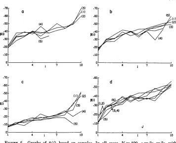
FIGURE 5.-Graphs of p ( i ) based an samples. In all cases, N = 100, si= 2s, = 2s, with samples, N,,, = 25 and nsam = IO. In (a), (b) and (c), the results are from 5 x 5 arrays, and

the selection coefficients are (1) s = 0.002; (2) s = 0.001; (3) s = 0; (4) s = -0.001; ( 5 ) s = -0.002. In (d), the curve numbers corresponding to the different cases are: (1) 5

x

5

array, s =0.002; (2) 5 x 5 array, s = 0.001; (3) 4 x 4 array, s = 0.002; (4) 4 X 4 array,

s = 0.001; ( 5 ) 5 x 2 array, s = 0.002; (6) 5 x 2 array, s = 0.001.

the samples than for the complete information. These graphs are also more variable than those based on complete information, because samples were taken every 50 generations. However, for a given sample size, there are no systematic differences between the curves for different selection coefficients.

As in the case of the occupancy distribution, we can consider the dependence of samples of a given type when the actual populations are different. Although only a limited set of such cases can be examined with the present simulation program, there does not appear to be strong dependence on the actual number of demes when the same number of demes are sampled and the geometric arrangements of the deme are similar. This is illustrated for one set of cases in Figure 5d. There is some variation in the results for all of the cases, but there seems to be no systematic dependence on the actual number of demes.

DISCUSSION

(16)

518 M. SLATKIN

tion, Pi, provides information about the number of demes in which the mutant is found, and the conditional average frequency,

p(

i)

,

or other measures of the mutant frequency distribution conditioned on the occupancy number, provides information about the extent of local differentiation for different occupancy numbers. The properties of these two types of statistics were found from a computer simulation program because the complete analytic solution for a model of a subdivided population does not seem possible using available methods. However, it is possible to consider certain extreme cases for which some approxi- mate analytic results can be obtained to determine whether the simulation results are consistent with those results.

The two extreme cases that can be treated analytically are those of small and large rates of migration, as measured by the parameter m in the simulations. NAGYLAKI (1 980) showed that, as migration becomes strong relative to selection and genetic drift, a diffusion model for a subdivided population converges on a diffusion model for a single panmictic population. NAGYLAKI observed that, if the migration is conservative i n the sense that the average gene frequencies are unchanged by the migration process, the effective size of the panmictic population is the same as the total number of individuals, nN. With equal derne sizes, a symmetric migration matrix is conservative, but in the simulations, the migration matrix was not symmetric.

NAGYLAKI

showed that when the migration matrix is not conservative, the size of the panmictic population can differ from the total number of individuals. However, since only the qualitative features of the panmictic limit are of importance here, and since the migration matrix used in the simulations is nearly symmetric, the results for a panmictic population of size nN will be discussed. The results for some simulations made using a symmetric migration pattern did not differ qualitatively or quantitatively from those presented above.

I n a panmictic population, the identification of individuals with demes is purely arbitrary and does not affect the mutant frequency. However, in a panmictic population of size Nn , it is possible to define a n occupancy distribution by choosing n groups of N individuals randomly each time a sample is taken. If the frequency of the mutant in the population is x, then there are 7 = 2 N x

copies of the mutant, and the occupancy distribution, given r-the probability that the mutant will be found in exactly i of the n groups of individuals-can be found from elementary combinational considerations to be

where

( j )

is the usual binomial coefficient.

The probability that the mutant will be found at frequency x is related to the distribution of sojourn times of a mutant, which is, for the case of no dominance,

1

(17)

MUTANT ALLELE DISTRIBUTION 519

(EWENS 1969, p. 60). The sojourn time,

t(x)dx

is the expected time that a new mutant will spend in the frequency interval

(z,x

+

d z ) before it is either lost of fixed.

The simulation model as described previously is a model of recurrent events

(FELLER

1957, Ch. 13), because each time a mutant is lost or fixed, a new mutant is introduced. For a model of a panmictic population defined as a recurrent processes in the same manner as the simulations, the probability that the mutant frequency is in the interval

(x,x

+

dx)

,

given that the process is sampled at a randomly chosen time is t ( z ) / i , where

t

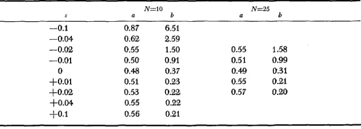
is the average time to loss or fixation of the mutant. Therefore, in the large migration limit of large migration rates, the occupancy distribution that would be expected is

While this function cannot be expressed in closed form, it is not very diffi- cult to evaluate numerically, at least for small values of n and N . A program was written to compute Pi from equations (1) through (3), and the computed Pi was fit to a beta distribution, using the same method as was used for the Pi generated by the simulations. The results are shown in Table 6. We can see the same trend in the values of the two parameters of the beta distribution as was found for the simulation results. It was also found that the fitted beta distributed deviated systematically from the computed Pi in the same way as for the simulation results for larger migration rates. For positive selection coefficients, the beta distribution was somewhat larger than Pi for the intermediate occupancy numbers. The deviations were much smaller for negative selection coefficients.

In the other extreme, that of small migration rates, the gene flow between populations is assumed to be sufficiently infrequent that once a mutant reaches a particular deme, it will become lost or fixed independently of the migration process. For a given deme size, N , and a given set of selection coefficients, s1 and

TABLE 6

Values of a and b for a beta distribution fitted to Pi computed from equations ( I ) and ( 2 ) f or the limit of large migration rates

N=iO N=25

5 a b a b

-0.1 0.87 6.51

-0.04 0.62 2.59

-0.02 0.55 1.50 0.55 1.58

-0.01 0.50 0.91 0.51 0.99

0 0.48 0.37 0.49 0.31

+O.Ol 0.51 0.23 0.55 0.21

+O.oZ 0.53 0.22 0.57 0.m

+O.W 0.55 0.22

+O.l 0.56 0.21

~~

(18)

520 M. SLATKIN

se, the probability of fixation of a mutant that is introduced in a single copy is known approximately from diffusion theory to be

U = J',/""G(x)dz/S1,G(x)dx

(4)

where

G ( X ) =

MP{

2N [2 (~1-~2) Z+ (~2-2~1)

2'1

} ( 5

1 KIMURA

(1962). Also, if the mutant is fixed in a deme and a single copy of the other allele is introduced, the probability of loss of the mutant is

U = G(z)ds/J1,G(z)dz

.

1 - 1 / 2 N

In the low migration limit, the population at any time can be thought of as a set of demes, some of which are fixed for the q u t a n t and the rest fixed for the other allele. The low migration rate causes the time scale of the process to be expanded sufficiently that the time when any deme is polymorphic occupies such a small fraction of the total time that it can be ignored.

In

t h i s limit, the population resembles a haploid Moran model

(MORAN

1962) in that each deme makes a transition from one state to the other, with rates depending on the states of the rest of the demes. The model of a subdivided population in the low migration limit is not the same as a Moran model since only those demes that send migrants to a particular deme can cause that deme to make a transition from one state to the other. However, it was shown elsewhere (SLATKIN

1980) that in the low migration limit, the model in some cases can be made formally equivalent to a haploid Moran model with selection coefficients

1

and

U/U on the two haplotypes. Using

a

diffusion approximation to the Moran model,

the sojourn times can be obtained from (2), which with a change in notation yields

t(r)

r

l-exp (--2nz (1-Y)

1 /

[Y

( 1 7 )

1

(7)

t ( Y > cc l/Y ( 8 )

for U#U, where z = ( U-U) /( U + U )

,

and

for U = U (i.e., s2 = 0).

The expected occupancy distribution is obtained from (7) or (8) by renormal- izing. Note that z in (7) depends on the ratio U/V, which is independent of sl, the selection coefficient on the heterozygote.

We see, then, that in the limits of both large and small migration rates, the expected occupancy distribution is very similar to a U-shaped or J-shaped beta distribution, but the functional form is not exactly that of the beta distribution. It seems reasonable that the occupancy distribution for intermediate levels of migration, for which analytic results cannot be obtained, should have the same character.

(19)

I I 1

1 4 7 10

I

I (2)

.so -

-40-

.20

-

. l o -

0 I

4 . 7 10

I

1

FIGURE 6.-Values of p ( i ) computed for the panmictic limit as discussed in the text. The curves corresponding to the different selection coefficients are: (1) s=O.1; (2) s = 0.04; (3)

For (a), n = IO, N = 10, and for (b), n = 10 and N = 25.

s 0.02; (4) s = 0.01; (5) s = 0; (6) s = -0.01; (7) s = -0.02; ( 8 ) S = -0.04; (9) s =-0.1.

the same type of argument applies as well to other statistical measures of the conditional distribution. In the limit of large migration rates, when the population is effectively panmictic, we can compute

p

(i)

from (1 )

.

First, we note that if both

i,

the occupancy number, and r, the number of copies of the mutant in the population are given, then the average frequency of the mutant in those

i

demes must be r / 2 N i . If we denote this quantity by p ( i l r ) , we have from elementary probability theory

p ( i )

=+

p(ilr)Pr(rji)

,

(9)

(20)

522 M. SLATKIN

bility is related to P r ( i l r ) , which is related to equation (1) by the usual formula

P r ( r l i ) =

Pr(ilr)Pr(r)/Pr(i)

.

(10)

Finally, P r ( i ) =

Pi,

by definition, and P r ( r ) is obtained from the distribution of sojourn times, so that we have sufficient information to compute

p(i)

in equation (9). The resulting formula cannot be expressed i n a simple form but can be computed numerically. Results for two sets o€ cases are shown in Figure 6. Clearly, the results for the large migration limit have exactly the pattern found in the simulation. There is almost no dependence of

p ( i )

on the selection coefficients, except at the maximum occupancy number, What dependence there is on the selection coefficients decreases rapidily as local deme size, N , increases. I n the small migration limit, we would not expect to find any dependence

of

p ( i ) on the selection coefficients. For extremely small migration rates the

mutant is either fixed or absent in each deme. Thus, the distribution of the mutant conditioned on the occupancy number is known and is independent of the selection coefficients. It is clear from the simulations that this limit was not approached even for the smallest migration rates ( N m = 0.1). It was not feasible to run a sufficient number of replicates for smaller migration rates.

Thus, in the limit of both large and small migration rates, there should be little or no dependence of p ( i ) and the other statistics on the selection coefficients acting on the mutant. The results from the simulations for intermediate migration rates are consistent with these analytic results.

CONCLUSIONS

The goal of this study is at least partially reached. It is possible using a computer simulation model to find relatively simple properties of the spatial distribution of a mutant allele introduced into a subdivided population. Additional assumptions must be made before these results can be applied to data from natural populations. The simulation program models only a two-allele system at a single locus. The process of recurrent mutation was not considered. To apply these results, it would be necessary to show that the same patterns are found when the mutation process and multiple alleles are included. Those will be included in a subsequent study. This study shows the kinds of patterns to be looked for in more complicated simulations.

I thank J. FBLSENSTEIN for numerous helpful discussions of this topic, The research was supported by research grants from the Public Health Service (R01-GM22523) and the National Science Foundation (DEB-7827045), and I have been supported by a Public Health Service Research Career Development Award (K01-GM0018) during the course of this research.

LITERATURE CITED

BOORMAN, S. A., 1974 Island models for takeover by a social trait facing a frequency-dependent selection barrier in a Mendelian population. Proc. Natl. Acad. Sci. U.S. 71: 2103-2107.

164: 362-379.

(21)

MUTANT ALLELE DISTRIBUTlON 523

CRUMP, K. S. and J. H. GILLESPIE, 1976 The dispersion of a neutral allele considered as a branching process. J. Appl. Prob. 13: 208-218. __

,

1977 Geographical distribution of a neutral allele considered as a branching process. Theor. Pop. Biol. 12: 10-20.

EWENS, W. J.. 1969 FELLER, W., 1957

JOHNSON, N. L. and S. KOTZ, 1970

KIMURA, M., 1953

Population Genetics. Methuen & Co., London.

An Introduction to Probability Theory and Its Applications. John Wiley &

Distributions in Statistics: Continuous Uniuariate Distribu-

Sons, New York.

tions-2. Houghton Mifflin Co., Boston.

“Stepping stone” model of population. Ann. Rep. Natl. Inst. Genetics, Misima, Japan: 3: 62-63. -- , 1962 On the probability of fixation of mutant genes in a population. Genetics 47: 713-719.

LEWONTIN, R. C. and J. KRAKAUER, 1973 Distributions of gene frequency as a test of the theory of the selective neutrality of polymorphisms. Genetics 74: 175-195.

MARUYAMA, T., 1970 On the fixation probability of mutant genes i n a subdivided population. Genet. Res., Camb. 15: 221-225.

-

, 1971 An invariant property of a structured population. Genet. Res., Camb. 18: 81-84, --, 1972 Some invariant properties of a geographically structured finite population: distribution of heterozygotes under irrever- sible mutation. Genet. Res., Camb. 20: 141-149. -, 1974 A simple proof that certain quantities are independent of the geographical structure of population. Theor. Pop. Biol.

5: 148-154.

The Statistical Processes of Euolutionary Theory. Clarendon Press, Oxford.

Decay of genetic variability in geographically structured populations. Proc. Natl. Acad. Sci. U.S. 74: 2523-2525. -, 1980 The strong-migration limit in geographically structured populations. J. Math. Biol. (in press).

NEI, M. and T. MARUYAMA, 1975 Lewontin-Krakauer test for neutral genes. Genetics 80:

395.

POLLAK, E., 1966 On the survival of a gene in a subdivided population J. Appl. Prob. 3:

142-155.

ROBERTSON, A., 1975

SAWYER, S. and J. FLEISCHMAN, 1979

MORAN, P. A. P., 1962

NAGYLAKI, T., 1977

Remarks on the Lewontin-Krakauer test. Genetics 80: 396.

Maximum geographic range of a mutant allele considered as a subtype of a Brownian branching random field. Proc. Natl. Acad. Sci. U.S.

76: 872-875.

Fixation probabilities and fixation times in a subdivided population. Evolu- tion (in press).

The spatial distribution of transient alleles in a subdivided population: a simulation study. Genetics 89 : 793-810.

Migration and mutation in stochastic models of gene frequency change. J. Math. Biol. 5: 61-73.

Genetics of natural populations. VII. The allelism of lethals in the third chromosome of Drosophila pseudoobscura. Genetics 27 : 363-394.

Corresponding editor: M. NEI

SLATHIN, M., 1960

SLATKIN, M. and D. CHARLESWORTH, 1978

SVED, J. -4. and B. D. H. LATTER, 1977