A deep learning approach to real-time short-term trafﬁc speed prediction with spatial-temporal features

(1)

University of Windsor University of Windsor

Scholarship at UWindsor

Electronic Theses and Dissertations Theses, Dissertations, and Major Papers

2019

A deep learning approach to real-time short-term traf

fi

c speed

A deep learning approach to real-time short-term traf c speed

prediction with spatial-temporal features

Sindhuja Gutha University of Windsor

Follow this and additional works at: https://scholar.uwindsor.ca/etd

Recommended Citation Recommended Citation

Gutha, Sindhuja, "A deep learning approach to real-time short-term traffic speed prediction with spatial-temporal features" (2019). Electronic Theses and Dissertations. 7704.

https://scholar.uwindsor.ca/etd/7704

This online database contains the full-text of PhD dissertations and Masters’ theses of University of Windsor students from 1954 forward. These documents are made available for personal study and research purposes only, in accordance with the Canadian Copyright Act and the Creative Commons license—CC BY-NC-ND (Attribution, Non-Commercial, No Derivative Works). Under this license, works must always be attributed to the copyright holder (original author), cannot be used for any commercial purposes, and may not be altered. Any other use would require the permission of the copyright holder. Students may inquire about withdrawing their dissertation and/or thesis from this database. For additional inquiries, please contact the repository administrator via email

(2)

A deep learning approach to real-time short-term traffic

speed prediction with spatial-temporal features

By

Sindhuja Gutha

A Thesis

Submitted to the Faculty of Graduate Studies

through the School of Computer Science

in Partial Fulfillment of the Requirements for the

Degree of Master of Science

at the University of Windsor

Windsor, Ontario, Canada

2019

c

(3)

A deep learning approach to real-time short-term traffic speed prediction with

spatial-temporal features By

Sindhuja Gutha

APPROVED BY:

H. Maoh

Department of Civil and Environmental Engineering

X. Yuan

School of Computer Science

M. Kargar, Co-Advisor

J. Chen, Advisor

(4)

DECLARATION OF ORIGINALITY

I hereby certify that I am the sole author of this thesis and the intellectual content of this

thesis is the product of my own work and that no part of this thesis has been published or

submitted for publication.

I certify that, to the best of my knowledge, my thesis does not infringe upon anyones

copyright nor violate any proprietary rights and any ideas or techniques and all the

as-sistance received in preparing this thesis and sources have been fully acknowledged in accordance with the standard referencing practices. Furthermore, to the extent that I have

included copyrighted material that surpasses the bounds of fair dealing within the meaning

of the Canada Copyright Act, I certify that I have obtained a written permission from the

copyright owner(s) to include such material(s) in my thesis and have included copies of

such copyright clearances to my appendix.

I declare that this is a true copy of my thesis, including any final revisions, as approved by my thesis committee and the Graduate Studies office, and that this thesis has not been

(5)

ABSTRACT

In the realm of Intelligent Transportation Systems (ITS), accurate traffic speed prediction

plays an important role in traffic control and management. The study on the prediction of

traffic speed has attracted considerable attention from many researchers in this field in the

past three decades. In recent years, deep learning-based methods have demonstrated their

competitiveness to the time series analysis which is an essential part of traffic prediction.

These methods can efficiently capture the complex spatial dependency on road networks and non-linear traffic conditions. We have adopted the convolutional neural network-based

deep learning approach to traffic speed prediction in our setting, based on its capability of

handling multi-dimensional data efficiently. In practice, the traffic data may not be recorded

with a regular interval, due to many factors, like power failure, transmission errors, etc., that

could have an impact on the data collection. Given that some part of our dataset contains a

large amount of missing values, we study the effectiveness of a multi-view approach to im-puting the missing values so that various prediction models can apply. Experimental results

showed that the performance of the traffic speed prediction model improved significantly

after imputing the missing values with a multi-view approach, where the missing ratio is

(6)

DEDICATION

Dedicated to my parents Shobha and Ravinder Reddy, my

(7)

ACKNOWLEDGMENT

I would like to sincerely express my most profound gratitude towards my supervisors Dr.

Jessica Chen and Dr. Mehdi Kargar for providing invaluable guidance, continuous support

and motivation.

I would also like to thank my thesis committee members Dr. Hanna Maoh and Dr.

Xiaobu Yuan for their valuable guidance, comments and suggestions that added more value

to my thesis work.

I would like to take this opportunity to sincerely thank Dr. Mina Maleki. As my guide

and mentor, she has taught me more than I could ever give her credit for here. I would like

to thank my mentors Dr. Hanna Maoh and Dr. Mina Maleki from my research at

Cross-Border Institute (CBI) for giving me the opportunity to be a part of this institute for my

thesis work.

Also I would like to thank all the staff of Graduate Society of Computer Science for their kindness. I am extending my thanks to all my friends and colleagues who supported and

helped me during this period.

On a personal note, I would like to express my deepest gratitude to my parents, my

husband, my inlaws and my sister for their immense support from the very beginning.

Collectively, all of their support and guidance has enabled me to successfully complete

(8)

LIST OF TABLES

3.1 Summary on traffic prediction during normal and unusual traffic conditions 36

3.2 Summary on traffic prediction considering various traffic patterns . . . 37

3.3 Summary on methods for network-wide traffic prediction . . . 54

3.4 Summary on methods using CNN for traffic prediction . . . 55

4.1 Percentage of missing values in each location . . . 60

4.2 Sample records from raw Geotab data . . . 62

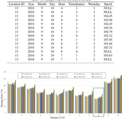
4.3 Sample of processed GEOTAB data . . . 63

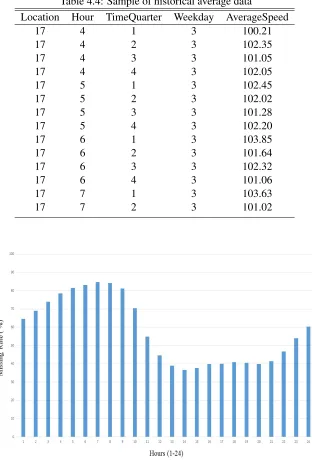
4.4 Sample of historical average data . . . 64

4.5 An example of time series with length 20 . . . 67

4.6 An example showing speed profile with subsequence length 4 . . . 69

4.7 Speed count less than 70 . . . 77

4.8 Unusual traffic patterns . . . 79

5.1 Traffic speed prediction for 2 hours using CNN, LSTM, ANN models . . . 87

5.2 CNN recursive multi-step prediction - MAPE . . . 89

5.3 CNN single-step prediction- MAPE . . . 90

5.4 LSTM and CNN for single step prediction - MAPE . . . 91

5.5 CNN single-step prediction with mask - MAPE . . . 92

5.6 CNN model with weekday and hour - MAPE . . . 93

5.7 Comparison of different imputing methods for missing values - MAPE . . . 96

5.8 CNN model with different missing rates in train data - MAPE . . . 97

5.9 CNN model before and after filling the missing values in train data - MAPE 98 5.10 Atypical sequence information where historical speed- actual speed >0 -Temporal . . . 99

5.11 Atypical sequence information where historical speed- actual speed>10 -Temporal . . . 99

5.14 CNN recursive multi-step prediction with dynamic- kNN - MAPE . . . 102

5.15 Real-time prediction with 10% missing rate . . . 103

(11)

LIST OF FIGURES

1.1 Representation of missing data . . . 4

2.1 A Neuron . . . 8

2.2 Feed Forward Neural Networks . . . 9

2.3 a) Convolutional Neural Networks . . . 15

2.4 b) Convolutional Neural Networks . . . 15

2.5 CF Temporal . . . 17

2.6 CF Spatial . . . 19

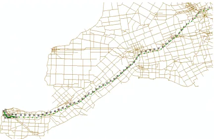
4.1 72 Locations across the 401 Highway . . . 59

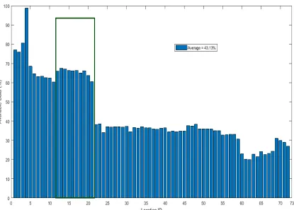
4.2 More percentage of available data in locations 12 to 21 . . . 61

4.3 Locations 12 to 21 across highway 401 . . . 62

4.4 Less percentage of missing values in October . . . 63

4.5 Percentage of missing values in each hour . . . 64

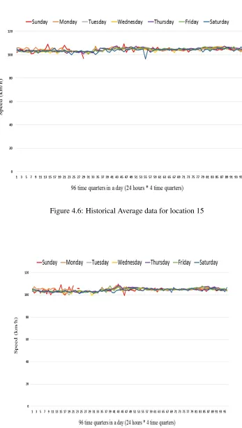
4.6 Historical Average data for location 15 . . . 65

4.7 Historical Average data for location 19 . . . 65

4.8 Type 1 missing pattern . . . 70

4.12 Multi View . . . 72

4.13 Temporal unusual traffic pattern . . . 74

4.14 Unusual traffic pattern in location 16 . . . 75

4.17 Traffic patterns in all locations . . . 78

4.18 Recursive model prediction with dynamic k-value . . . 81

4.19 Real time model prediction . . . 82

5.1 Traffic speed prediction using CNN with different number of time lags . . . 86

(12)

LIST OF SYMBOLS

Symbol Definition

ANN Artificial Neural Networks

DNN Deep Neural Networks

RNN Recurrent Neural Networks

CNN Convolutional Neural Networks

LSTM Long short term memory neural networks GRU Gated Recurrent Units

SVR Support Vector Regression

CF Collaborative Filtering

SQL Structured Query Language

kNN k Nearest Neighbors

SF Spatial Features

(13)

Chapter 1 INTRODUCTION

1.1 Motivation

In the transportation field, accurate traffic prediction plays an important role in traffic

control and management, and it has gained considerable attention from transportation

re-searchers and practitioners. Analyzing, understanding and estimating future traffic condi-tions can certainly help road users to settle on better travel choices, improve the quality

of traffic operations and reduce traffic congestion. And, to support traffic managers in

allocating resources systematically and help people with complete traffic information,

un-derstanding traffic movement for the whole road network is of great significance [1]. Due

to computational complexity caused by road network topology, spatial correlations in

traf-fic data expanding on a two-dimensional plane, long term prediction to reflect congestion propagation, large-scale network traffic speed prediction is challenging [2]. The main aim

of our research work is to predict traffic speed at multiple locations simultaneously on

high-way 401 in Canada. This highhigh-way is one of the busiest corridors in North America. This

highway extends from Windsor in the west to the Ontario Quebec fringe in the east [3].

Also, this highway connects to the Ambassador bridge which is an essential single freight

link in the Canada-US trade relationship. It carries about 2.5 million trucks for each year, accounting for about 20% of Canada-US trade [4].

In the real-time, traffic speed may be low during a certain time of the day (peak hours

traf-fic) and usually, weekday traffic is different from weekend traffic. Features extracted from

this type of information which depends on time are called temporal features. Similarly,

(14)

from this type of information are called spatial features. And, sometimes the planned

in-cidents such as road maintenance works/construction works affect the traffic conditions. Sometimes unplanned incidents and accidents result in atypical traffic conditions. In

addi-tion to the spatial and temporal features, our research work also focuses on atypical traffic

conditions because the identification of these conditions can help in better traffic

forecast-ing, provide information to transportation engineers for better road network design and can

be used to reduce congestion. Atypical traffic speed can be a significant drop in speed on a

section of highway.

These days a large amount of real-time traffic information is available due to the

de-velopment and deployment of the latest technologies in intelligent transportation systems

(ITS). Loop detectors, Global Positioning Systems (GPS) devices and Remote Traffic

Mi-crowave Sensors (RTMS), etc. can readily collect traffic data. However, the traffic data is

often missing regardless of the technology used. Reasons for incomplete traffic data can be

power failures, errors in transmitting the data, hardware or software malfunctions. In many

traffic-related times series datasets, missing data are prevalent [5]. Efficient data analysis depends on the quality of data, and the missing data affects the performance of data

anal-ysis like traffic forecasting. The performance of several forecasting models will reduce if

missing data is present. Even in our dataset, most of the locations contains around 40%

of missing data and in some locations it is more than 90%; hence it is necessary to impute

the missing data with efficient imputation models. In our dataset, the speed information is

collected through cutting edge GPS based vehicle tracking devices which are installed in vehicles. If the vehicles with GPS vehicle tracking devices do not go through any location

and during any timestamp then the speed will not be recorded during that timestamp and

location. Because of this, we have missing information in our dataset. The missing data

problem is challenging especially when the missing data percentage is more. Attributing

(15)

tem-poral features and study the effects of missing data on the performance of traffic prediction

, profoundly motivated the present research work.

This thesis first focuses on imputing the missing values based on the Multiview approach

[5, 6]. For local temporal and local spatial views we considered collaborative filtering

techniques and simple average techniques, and for the global temporal and global spatial

views we used the historical average data. Once the complete dataset is available (i.e.,all

missing values are imputed), we build the traffic speed prediction model based on CNN [2]

and predict the network-wide traffic speed for the next two hours.

The data used in this thesis is collected by GEOTAB and provided to us by the

Cross-Border Institute at the University of Windsor. The obtained dataset contains traffic speed

records across 72 locations on the 401 Highway from November 2017 to October 2018.

The traffic speed data is aggregated in 15-minute time intervals. We used the first eleven

months of data for training various models and retain one-month data, i.e., October 2018

data for testing.

The network-wide traffic speed prediction in this research work help in travel time pre-diction on specific locations on highway 401, crossing time prepre-diction over one of the

busiest US Canada bridges, the Ambassador Bridge.

1.2 Research Objective & Solution Outline

This research outlines the prediction of traffic speed using spatial and temporal features across highway 401 at specific locations for the next two hours in the future. The

accu-racy of the traffic speed prediction depends on many factors like the amount of available

historical data, how well the patterns are represented in the historical data, which model is

suitable for the nature of the dataset, etc. Our dataset contains more than 40% of missing

(16)

forecast-ing model. Hence, our first task is to impute the missforecast-ing values. Once the complete dataset

is available, we build the traffic speed prediction model and predict the traffic speed. The problem statement for the missing value imputation in traffic time series data can be

de-fined as follows: Given data = [l₁,l₂,l_i,....,l_p] with p locations, Where eachl_i= [t1, t2,....,tq]

represents the time series of traffic speed during q time intervals from the sensorl_i. The

un-available values in this data are called missing values. Based on the un-available information,

missing value imputation models predicts the unavailable data. In Figure 1.1, X represents

the missing value. Predicting the future traffic speed of the road segment based on the

his-Figure 1.1: Representation of missing data

torical observations is called Traffic speed prediction. Traffic speed prediction comes under

supervised learning which means we must train the model with input/output pairs and the

trained model would predict the output for the given input. Such problems come under the

category of regression problems. The input data for predicting the traffic speed at single

location is w(time lags) historical time steps as shown in the below equation

S_i= [S_i,t−1,Si,t−2, . . .Si,t−w]

(17)

locations. Sometimes traffic congestion may propagate from far away locations. In this

study, we consider these network-wide impacts into account. Hence the input data for the prediction model is the network-wide traffic speed. We have p locations, and we need to

predict the traffic speeds at future n time steps by using w time lags. This input speed data

is represented in the matrix format as shown in the below equation.

X_T =

         

S₁_,_t₋₁ S₁_,_t₋₂ S₁_,_t₋₃ . . . S₁_,_t₋_w

S₂,t−1 S2,t−2 S2,t−3 . . . S2,t−w

..

. ... ... . .. ...

SP,t−1 SP,t−2 SP,t−3 . . . SP,t−w          

The predicted output is represented in the matrix format as shown in the below equation.

Y_T =

         

S1,t S1,t+1 S1,t+2 . . . S1,t+n

S₂_,_t S₂_,_t₊₁ S₂_,_t₊₂ . . . S₂_,_t₊_n

..

. ... ... . .. ...

S_P,t SP,t+1 SP,t+2 . . . SP,t+n          

We have adopted the CNN based model for network-wide traffic speed prediction

be-cause CNNs can capture the spatiotemporal features of network traffic with a high

predic-tion accuracy [2]. The objective of this thesis is to impute the missing values and predict

network-wide traffic speed. The methods for assigning the missing values include collabo-rative filtering techniques, simple average and historical data.

1.3 Structure of thesis

The remaining part of this thesis is organized as follows:

(18)

for regression problems.

Chapter 3 briefly describes previous studies in the field of transportation for traffic pre-diction. Various machine learning models and their variations, and other similar approaches

for finding missing values are presented in this chapter. And works related to atypical

traf-fic patterns are summarized in this chapter. Several works related to predicting traftraf-fic speed

are included in this chapter.

Chapter 4 presents the primary contribution of this thesis and describes the

implementa-tion details of our approach. The significant contribuimplementa-tions of this research are :

• Implementing a multi-view approach for imputing missing values, a CNN

based model for network-wide traffic speed prediction with analysis on unusual

traffic speed patterns.

• Study the effects of missing data on the performance of traffic prediction.

• Implementing dynamic k-NN combined with CNN model.

• Real-time traffic speed prediction with missing data.

Chapter 5 reports the experimental results along with the detailed discussions.

(19)

Chapter 2 BACKGROUND STUDY

2.1 Artificial Neural Networks

Artificial neural networks (ANNs) have been used in various disciplines for solving

com-plex real-world problems. These are computing systems which are inspired by the

biolog-ical neural networks. In traffic prediction problems, they approximate a mapping function from input variables to output variables based on the historical data (training data). Deep

neural networks (DNNs) are ANNs with multiple layers between the input and output

lay-ers , and the set of mathematical operations are used to turn the input into the output. In

recent years, deep learning-based methods (such as LSTM, CNN) have demonstrated its

competitiveness to the time series analysis which is an essential part of traffic prediction.

These methods can handle the complicated nonlinear spatial, and temporal correlations and the different variants of these methods have been used for traffic speed prediction.

The structure of the ANN is analogous to the structure of a biological neural system. It

is composed of multiple processing units (called artificial nodes or neurons) connected in

consecutive layers to work together and produce the final output. ANNs have a fantastic

information processing characteristics such as non-linearity, fault and failure tolerance,

ro-bustness, high parallelism, and their capability to generalize [7]. In transportation research, ANN models have a long application history. Compared to the classical statistical models,

ANN models can capture the nonlinear relationship between dependent and independent

(20)

A Neuron in the context of transportation

The basic building block of ANN is the neuron. It can be considered as a computational unit which receives input and process that input to produce the output. Each input has

some weight. This processing can be the simple summation of products of inputs and their

weights or the summation of products of inputs and their weights passed through some

activation function. The activation function is to provide the non-linearity to ANNs. The

activation function produces the output in the desired range such as 0 to 1 or -1 to 1 . For

example, the logistic activation function produces the output in the 0 to 1 range [9]. Suppose the last one-hour traffic speed information is used to predict the speed in the next

15 minutes and the traffic speed data collected is for every 15 minutes. In this scenario, the

number of input features for the neuron is four , and the output is one.

In Figure 2.1, x1, x2, x3, x4 are input features and their respective weights are w1, w2,

w3, w4. w0 represents the bias value and y represents the output value.

Figure 2.1: A Neuron

Output value y is computed by the below equation which is the function of sum of

(21)

ˆ

y= f(W X+w₀) (2.2)

f(x) =φ(x) (2.3)

whereφ represents the activation function

If f(x) =x, the output value of the neuron y=W X+w₀ which is the equation for linear

regression, here the activation function is identity function.

If f(x) =sigmoid(x), the output value of the neurony=₁₊_e−₍_{W X}1 ₊_w

0) which is the equation

for logistic regression, here the sigmoid is the activation function.

The parameters in the above model (single neuron) are weights(W) and the bias values(w0).

These values are learned from the training dataset. Artificial neural networks are just the

combination of many such neurons in multiple consecutive layers which are called hidden

layers. These neurons are connected in such a way that they can process the information together and solve complex problems.

2.1.1 Feed Forward Neural Networks

In this neural network, information flows in one direction only from the input layer to

the output layer and the neurons from one layer are connected to all the neurons in the next

following layer as shown in Figure 2.2.

(22)

The neurons are connected by weighted connections, which carry the information from one

layer to the subsequent layer. These neural networks consist of one or more hidden layers. They can approximate nonlinear functions by adapting nonlinear activation functions. The

model can be called a deep neural network if it has two or more hidden layers.

Training of the neural network model A common objective for ANN in regression

problems is to minimize the sum of squared errors which means to reduce the error

be-tween the actual values and predicted values (Equation 2.4). To achieve this objective, we

need to train the neural network model. Training means adjusting the parameters of the model from the training dataset. In other words, it means estimating the best set of

param-eters i.e., weights and bias of the model such that there will be less error in prediction. A

backpropagation approach is typically used to train the neural network model [8] and it has

been applied in predicting traffic speed. A number of other optimization algorithms were

also developed to achieve this goal like the Genetic algorithm etc.

J=1/n n

∑

i=1

(yi−yˆi)2 (2.4)

The backpropagation algorithm is a supervised learning algorithm which is based on a

gradient descent technique to train neural networks. The primary goal of this gradient

descent method is to minimize the error function (which is also called as a cost function or

objective function) by adjusting the parameters in the model. In each training step, error

function (Equation 2.4) is calculated, and the parameters(weights and bias) of the neural network are adjusted by back-propagating the error from the output layer to the input layer

so that the error in the next iteration will be reduced. In other words, the training process

involves running the model in both directions. First, we get the prediction using the current

model parameters by forward pass which means we pass the input to the input layer and

(23)

calculate the error function (Equation 2.4). Then we calculate the partial derivative of the

error function (gradient). In the next step we update the parameters of the model along the opposite direction of a gradient to minimize the error function value. Once the model

is ready (error rate converged or reached maximum number of epochs), we can use it for

prediction.

Gradient descent techniqueIt is a popular optimization method which is used to find

maxima/ minima of a differentiable function. It minimizes the error function by iteratively

updating the parameters in small steps by using the direction of the gradient of the error function w.r.t. to the parameters.

Let W be the set of parameters

Step 1: Initialize W randomly

Step 2: Update the parameters based on the below equation

W hile not converged or till the maximum number o f epochs:

W =W−η∗gradient(cost f unction,trainingdata,w)

Hereη is the learning rate which decides how much the parameters are updated in each

step and one epoch means all training samples are passed through the neural network only

once.

There are three variants of gradient descent. The difference between these three is in

how much of the total training data is used to compute the gradient of the error function

(also called loss or cost function) [10].

• Vanilla gradient descent: The gradient of the cost function w.r.t. to the

pa-rameters is computed using the entire training dataset. Here to perform just one

update, the gradients for the whole dataset are calculated. It can be very slow when the size of the dataset is large.

(24)

sample. For large datasets, redundant computations are performed in vanilla

gradient descent as gradients are recomputed for similar examples. SGD solves this by performing one update at a time. It is much faster in learning, but the

frequent updates can cause the cost function to fluctuate more.

• Mini-batch gradient descent: Parameters are updated for every mini-batch

of training samples. It requires less memory and leads to more stable

con-vergence. This batch size is one of the hyperparameters in training the neural

network model.

There are several gradient-based optimization techniques such as Adagrad, Adadelta,

RMSprop, Adam, AdaMax, etc. widely used by Deep Learning community [10] . And

also various activation functions exist such as sigmoid, tanh, ReLu, etc. In this study, for all the neural network models we use the Adam optimization algorithm and the ReLu

activation function in CNN model, tanh activation function in LSTM model.

2.1.2 Recurrent Neural Networks

The traditional feedforward neural networks do not consider the temporal information

for time series inputs. For example, if we consider four previous time lags to predict speed

in the next time interval, then these four-time lags are regarded as independent features and the temporal information between these time lags is not considered. Recurrent neural

networks can learn the temporal information; hence they are suitable for dealing with time

sequences. RNN hidden units receive feedback from the previous state to current state [11].

RNNs use the context information from previous time steps, which is usually referred to

as memory. Because of this capability, they can capture flexible temporal dependencies

(25)

and the final output not only depends on the current input but also depends on the previous

hidden layer output.

These networks were initially used for language models. RNNs unfold into the very

deep feedforward neural networks with more time lags. Because of this, the gradients of

the network may vanish or explode. In other words, if the time span becomes longer, the

accuracy of the network may reduce due to the vanishing gradient and exploding gradient

problems. The neural network models LSTM and GRU (Structures of RNN) were proposed

to solve this problem.

LSTM model was proposed [12] to overcome the vanishing gradient problem in

tradi-tional RNNs. Vanishing gradient problem prevents the RNNs from capturing the long-term

dependencies. A mechanism referred to as a gating mechanism in this model makes the

de-cisions about updating its memory. Typical LSTM unit consists of an input gate, an output

gate, a forget gate and a cell. Input gate decides what amount of new information should

be stored in the memory; the output gate decides what information in the memory is used

to calculate the output of the LSTM unit; the forget gate decides what information should be deleted from the memory. Here the cell represents the memory.

Due to this forget gate, the method can decide when to forget certain information. Output

layer of the LSTM cell is the linear regression layer. By maintaining a memory state of the

cellc_t, LSTM can learn sequential correlations. The output of the memory cell is controlled

by the output gate.

Hidden layers are treated as memory units in LSTM network. They can learn the corre-lations within time series in both short term and long term. The center of the LSTM unit

is the memory cell, and the state of it is denoted byc_t. Input datas_t (traffic speed at time

interval t) and output of the LSTM cell in the previous time intervalh_t₋₁ are the inputs of

(26)

calculated using the below equations.

it=σ(Wi,sst+Wi,hht−1+bi) (2.5)

f_t =σ(Wf,sst+Wf,hht−1+bf) (2.6)

o_t =σ(Wo,sst+Wo,hht−1+bo) (2.7)

˜

ct=tanh(Wc,sst+Wc,hht−1+bc) (2.8)

c_t=i_tc˜_t+f_tc_t₋₁ (2.9)

ht =ottanhct (2.10)

The input gate, the forget gate and the output gate at time interval t are denoted as i_t, f_t,

o_t. Tanh is a hyperbolic tangent function and o denotes Hadamard product. These both

functions are element-wise.

In another variant of LSTM, the input, output, and forget gates also look at the memory state of the cellct along withst,ht−1.

2.1.3 Convolutional Neural Networks

A CNN is an efficient image processing algorithm and achieved successful results in the

computer vision and image recognition fields [13].

Hidden layers in CNN architecture are convolution layers, pooling layers, fully

con-nected layers. Different filters (or kernels) in a convolution layer extracts different features.

These filters are set of weights which are learned through the training process to produce the output features. A pooling layer is usually applied after a convolution layer which

se-lects the essential features from the extracted features of the convolution layer , and due to

this, the model parameters are reduced tremendously. In traditional feedforward networks,

(27)

capture the local spatial features. The typical fully connected layers are used only in the

last stage after the convolution and pooling layers.

Figure 2.3: a) Convolutional Neural Networks

Figure 2.4: b) Convolutional Neural Networks

If we place the convolution filter on top of the input matrix, then the product between

the numbers at the same location in the input matrix and the filter are calculated and these products are summed up together to get a single number which is the convolution result

of this operation. Then the filter is moved to its right by one element (Here the stride is

(1,1) which means filter moves by one element to the right, one element to the down until

(28)

throughout the input matrix to get the final convolution result matrix. In the traffic context,

if the size of the input matrix is ten rows which represents the locations, eight columns which indicates time steps and 32 filters with size 3X3, then the convolution result is of

size 8 X 6 X 32 as shown in Figure 2.3. In Figure 2.3, input to the CNN model is the traffic

speed matrix with size 10 x 8 where we consider traffic speed data from 10 locations and

8 previous time steps(time lags) to predict the speed at 10 locations in the future time step.

Extracted features through set of filters from the input speed matrix will be the input to the

fully connected layers. The last layer in Figure 2.4 is with the identity activation function and predicts the final output for a given input.

2.2 Multi View Learning Approach

Collaborative filtering techniques are widely used in recommender systems. In

recom-mender system, the similar users make similar rating for similar items [14].

2.2.1 Temporal Collaborative Filtering

In the temporal view for traffic context, each traffic data point at ti is considered as an

item. Let p be the number of locations and traffic speed is represented by s; locations

are represented by i; timestamps are represented by j. The similarity between the two

traffic data points which are at two different timestamps can be computed according to the

Equation 2.11.

sim(tmiss,tj) =

1

s p ∑ i=1

(si,miss−si,j)2/p

(2.11)

(29)

2.12.

ˆ

s(tmiss) = w ∑ j=1

sj∗sim(tmiss,tj)

w ∑ j=1

sim(t_miss,t_j)

(2.12)

Herewis the window size, it provides the range in which traffic speeds should be consid-ered andtmissrepresents the timestamp at which traffic speed is missing. Here the missing

traffic speed (att_miss) is computed as the weighted average of traffic speeds which are in

the same location ast_miss. The weights are the similarities between two timestamps (t_miss,

t_j) at different locations.

Figure 2.5: CF Temporal

To fill the missing value att_j, we must compute the weighted average of traffic speeds

which are in the window range,t_j₋₂(w1) +t_j₋₁(w2) +t_j₊₁(w3) +t_j₊₂(w4)/ (w1+w2+w3+w4)

(30)

is the similarity of two-time stamps (t_j, t_j₋₁) at different locations,w3is the similarity of

two-time stamps (tj,tj+1) at different locations,w4is the similarity of two-time stamps (tj,

tj+2) at different locations.

2.2.2 Spatial Collaborative Filtering

In this view, the locations are considered as items. The similarity of two locations at

different timestamps can be calculated according to Equation 2.13.

sim(lmiss,li) =

1

s w ∑ j=1

(smiss,j−si,j)2/w

(2.13)

Here w represents the window size and si,j is the traffic speed at ith location and jth

timestamp. The Equation 2.14 computes the local variation in spatial view.

To predict the missing value at location l_i, the weighted average of all available data

points at various locations must be computed (same timestamp for locationl_iand all other

locations).

l_i₋₂(w1) +l_i₋₁(w2) +l_i+1(w3) +li+2(w4)/ (w1+w2+w3+w4)

Here w1 is the similarity between the two locations (li, li−2) at different time stamps

which are in the window range. Similarly w2 is the similarity between the two locations

(l_i,l_i₋₁) at different time stamps which are in the window range, w3 is the similarity between

the two locations (l_i,l_i₊₁) at different time stamps which are in the window range, w4 is

the similarity between the two locations (l_i,l_i₊₂) at different time stamps which are in the

window range.

ˆ

s(l_miss) = p ∑ i=1

si∗sim(lmiss,li)

p

∑ sim(lmiss,li)

(31)

Figure 2.6: CF Spatial

2.3 Regression techniques

2.3.1 K- Nearest Neighbours

The k-nearest neighbor’s algorithm is a supervised non-parametric technique used for

both regression and classification [15]. It is one of the most straightforward and efficient

machine learning algorithms. In the k-NN regression, we choose the k nearest neighbors

from the training dataset and compute the output as the average of these k nearest neighbors.

k-NN regression algorithm:

(32)

• Sort the training samples by ascending order

• Choose the first k nearest neighbors from this sorted array

• Compute the output by taking an average of these k nearest neighbors

Here the distance metric can be Euclidean or any other distance metric. There are various

types of k-NN regression models in which different weights can be assigned to neighbors

or for features in the sample. These algorithms are robust to noisy training data and can be

efficient if training data represents almost all patterns. However, it may take more time to compute the distances for each query sample when the training data size is huge.

2.3.2 Support Vector Regression

The support vector machines (SVM) are one of the popular supervised learning models

in machine learning which are used for classification and regression tasks. Authors [16]

proposed a version of SVM for regression, called as support vector regression (SVR). This

method constructs a hyperplane or a set of hyperplanes in a high dimensional space on training data. Later on, this hyperplane would help us in predicting the value. Two

bound-ary lines create a margin, and these are different from the hyperplane. The best hyperplane

represents the largest margin. The cost function for building the SVR model depends only

on a subset of training data; hence it is memory efficient. In summary, the SVR regression

model first maps the input onto a high dimensional feature space using nonlinear mapping

(33)

Chapter 3 LITERATURE REVIEW

This chapter gives a brief overview of the research work carried out for imputing the

miss-ing values and predictmiss-ing the network wide traffic speed prediction. A lot of research work

has been done in the both areas. Methods for imputing the missing values can be the

sim-ple mean value imputation or the comsim-plex spatial-temporal imputation methods. These

methods are also highly depend on the nature of dataset, amount of the available data, etc. In this section, we briefly introduce various methods used to impute missing values.

Various types of methods have been developed and different techniques are used as per

different application needs.

3.1 Related works on the imputation of missing values

Methods for imputing the missing data can be divided into three categories: interpolation

based, statistical learning based, and prediction based [17]. In interpolation-based methods,

we fill the missing data with an average or weighted average of historical data observations

either from the same sensor and same time in neighboring days or from the same sensor

and same time in other days with similar traffic pattern. In this category one of the popular

approaches to impute missing traffic data for a road segment is the historical average. In this method, the missing data point is imputed for a road segment based on the average

value of historical data corresponding to the same time interval and same location [18].

However, this approach performs poorly in the presence of unusual traffic conditions. The

most popular pattern matching interpolation methods are based on k-nearest neighbors

(34)

whole dataset [19]. The k nearest neighbors are similar traffic patterns in other days. The

performance of these approaches is affected by the availability of neighboring data.

Statistical learning-based methods try to take advantage of the statistical feature of

traf-fic data. These methods assume a special probability distribution from the available data

and the values which best fit the assumed probability distribution will be used to impute

the missing data. Markov Chain Monte Carlo (MCMC) imputation method [20] and

Prob-abilistic Principal Component Analysis (PPCA) based imputation methods are popular in

this category. The PPCA- based model combines two techniques: a) principal component analysis (PCA) which is used to separate the significant parts of the traffic data from the

unable to model parts. B) The second technique is maximum likelihood estimation (MLE)

which is used to estimate the missing values based on the obtained significant parts. In

other words, PPCA extracts the statistical characteristics of the available data and

indi-rectly builds the regression model. This model makes a reasonable trade-off between the

local predictability, periodicity and other statistical properties of the traffic data [21].

Au-thors [17] extended the probabilistic principal component analysis (PPCA) based imputing method by considering multiple sensors measurements. Experimental results show that the

temporal-spatial dependence is nonlinear, and it could be better retrieved by kernel

prob-abilistic principal component analysis (KPPCA) based method instead of PPCA method.

Overall if temporal- spatial dependence is appropriately considered, the imputing errors

can be significantly reduced. The KPPCA model is more powerful than the PPCA model

because it is less strict about the linear mapping assumption of PPCA model because it as-sumes a nonlinear relationship between an observed sample and a latent variable. Authors

in this paper compared the performance of these two methods for four different scenarios

with missing ratios 5% to 30%. In the first scenario, they collected the data from a single

detector for one month. The RMSE error value for these two methods is smaller than the

(35)

months), nearest historical imputing method (collected at the same daily point in the

near-est day) and spline interpolation method. However, the difference between the PPCA and KPPCA method is minimal. In the second scenario, the dataset is from a single detector,

but it is collected for three months. The error rate is unchanged in this scenario which

indi-cates that the imputing error cannot be reduced by feeding more data. In the third scenario,

one-month data is collected from three detectors. Error rates are decreased in this scenario

which shows the advantages of spatial dependencies in PPCA and KPPCA methods. The

fourth scenario is like the third one, but the influence of time lag is considered. In this one, KPPCA method is better than the PPCA method. Authors stated that the calculation time

of KPPCA method is more than PPCA. Hence, this method considering only spatial

depen-dence is highly recommended for online systems. In summary, the performance of PPCA

based methods are often better than the conventional methods although these methods have

a strong assumption on the data. Another group of approaches are based on regression

algorithms which include linear regression model, quadratic regression model, etc. To

cap-ture the relationship between neighboring sensors, authors in [22] used a linear regression model to impute missing traffic volumes and occupancies. Authors in this paper modeled

each pair of neighbors linearly and the parameters of the model are fixed based on the

historical data.

Prediction based methods use existing traffic prediction methods. Some of the famous

traffic prediction models are time series models based on the Auto-Regressive Integrated

Moving Average (ARIMA) model, Support Vector Regression (SVR), Artificial Neural Networks, etc. In these models value is predicted using the function which is formed from

historical data pairs (Input/ Output) [23]. Authors in [24] studied the effects of missing

data on ARIMA and neural network model performances. They developed two-hybrid

approaches. One is based on the self-organizing map (SOM) and ARIMA, and other

(36)

used. In SOM/ARIMA hybrid approach, a series of traffic patterns are classified using a

Self-Organised Map and then ARIMA model is associated with each SOM cluster. The SOM/MLP model was similar to the SOM/ARIMA model. Three other naive models were

also used for forecasting. The first one simply used the current traffic flow as the predicted

value. The second naive model assumes the linear relationship between the predicted,

present and the last traffic flows. In this study, SOM/MLP model achieved the best

fore-casting performance compared to all other models. To study the effects of missing data

on forecasting performance, missing data is generated randomly until 30%. Three meth-ods were used to deal with the missing data. The first method is the average value of data

used for forecasting, second is replacing the missing value with 0, and the third one is the

average of all traffic flow data. The first method showed the best results among all. The

second method is the worst option among all. And also, ARIMA models are more

sen-sitive to the percentage of missing data when compared to neural networks. Most of the

prediction models predict the data by considering a few current time lags before the value

to be predicted. In this scenario, they do not use the data after missing timestamp, and if the specified time lag data is missing, these prediction models fail to give the results.

In recent years, several machines learning based approaches have been proposed for

imputing missing traffic data. The data usually determine the form of the function in these

approaches. They try to take full advantage of the data. One of the popular machine

learning based approaches for imputing the missing values are tensor-based methods [25,

26]. In this paper [27] authors proposed a Bayesian probabilistic imputation framework for imputing the spatiotemporal traffic data. In this method, the Bayesian probabilistic matrix

factorization model was extended to higher order tensors and applied it for imputation tasks.

The performance of the method is evaluated by using a nine-week traffic speed dataset. The

spatiotemporal traffic data can be organized into a multidimensional array (road segment *

(37)

three different representations (A) Matrix (road segment * time series), (B) Third-order

tensor (road segment * day * time interval), and (C) Fourth-order tensor (road segment * week * day * time interval). The performance of different tensor-based approaches are

evaluated using these three representations. Through extensive experiments, this study

showed how different data representations affect imputation performance and proved that

data representation is an essential factor for model performance. And also showed that a

third order tensor structure outperforms the matrix and fourth order tensor representations.

The Kriging method can also be used for imputing the missing data. It was first devel-oped as an interpolation technique for geographical surfaces, it has become a representative

geostatistical approach to predict an unknown value at an unobserved location by adopting

various statistical assumptions and conditions in the modeling and has further advanced

to different kriging methods. Here the interpolation was formulated as a weighted sum of

the values of their known neighbors. The multivariate extension of kriging is Cokriging

which allows using secondary data sources to complement observed primary data. In this

study [28], authors employed ordinary and simple cokriging methods to use a secondary trac dataset for imputing the missing detector data. Using the information from multiple

data sources can improve the imputation results of the spatial-temporal cokriging approach.

Authors in this paper proposed two cokriging methods that exploit the existence of

spatial-temporal dependency in trac data and employ multiple data sources, each with

indepen-dently missing data, to impute high-resolution traffic speed data under dierent data missing

pattern scenarios. Consider secondary data sources only if they are highly correlated with the primary data to improve the prediction performance of cokriging. The cokriging

meth-ods may have the test errors if there is a relatively weak correlation between two data

sources. When the missing pattern follows not random in time and location pattern, using

secondary data sources with the simple cokriging can improve prediction results. The

(38)

the proportion of high-speed observations in the validation dataset of a higher missing rate

scenario increases. The overall imputation error decreases as the size of missing block increases, since these high-speed observations are like the mean of the RTMS data used

in this study. Overall, this paper provides a brief guidance of when and how to utilize

multi-source data for traffic speed data imputation using the real traffic datasets.

Clustering based approaches have also been proposed for imputing the missing traffic

data. Authors in this paper [29] proposed the method in which first the road segments with

similar traffic flow patterns are grouped through k-means clustering. In the next step, for each group of road segments, a deep learning model based on stacked denoising

autoen-coders is used to extract the spatial-temporal relationships between those road segments

and use this information for imputing the missing data points. Implemented experiments

show that under different missing rates, the imputation accuracy of the proposed method

is robust. In the proposed method, missing data is imputed collectively for a group of

road segments. An autoencoder is a neural network which has the same number of input

and output neurons. The input vector is reconstructed in this model. A denoising autoen-coder (DAE) is a variant of autoenautoen-coder for which corrupted input is passed during the

training process. In this model, the hidden layer learns the robust features underlying the

input data. For the training sample, some random entries in the input are masked with

zero. This training sample is considered as the incomplete traffic data with some missing

values. Each layer in the proposed method is pre-trained using a greedy layer-wise

ap-proach and to improve the imputation performance; the whole network is fine-tuned. The proposed method can impute the missing data on any road segment using the traffic flow

relationships with other road segments in the same cluster. Authors in this paper [30]

pro-posed a denoising stacked autoencoders (DSAE) model for imputing traffic flow data. This

model consists of two blocks, one is autoencoders (AEs) and the other one is denoising

(39)

cap-ture the statistical dependencies between the inputs. If DAEs are connected to form deep

networks, then such models are called stacked denoising autoencoders (SDAE). However, both DAE and SDAE can be used for cleaning or denoising the data. In this paper,

au-thors combined the DAE which is used for denoising the corrupted traffic data, with the

stacked AEs which help in extracting the features from high dimension traffic data. This

combination of models results in forming a deep learning model named DSAE which has

the advantages of both DAE and stacked AEs. Overall this model recovers the data through

statistical dependency learning and the feature extraction. The traffic flow data from PeMS aggregated in five-minute intervals is used in this paper. Traffic flow data for each day are

represented in the form of vectors. Each vector indicates whether it is a weekday or not.

Authors used a k means clustering method to group these vectors into weekdays and

non-weekdays. They assumed that vectors of the same date from different VDSs are similar

(same weekday property). So, there are two clusters, one with weekday pattern and the

other with the non-weekday pattern. A new corrupted vector is assigned to the closest

clus-ter based on the distance. Authors in this paper investigated 18 different scenarios for the model with different spatial (upstream, downstream, all other VDSs) and temporal factors

(weekdays and non-weekdays). Experimental results show that the model using all VDSs

data of weekdays and non- weekdays is the best. The proposed model is compared with

the history model, ARIMA and BP neural network model under the missing rates ranging

from 5% to 50%. The experimental results show that the imputation accuracy is better in

the proposed model. Also, authors in this paper show the consistency of the imputed data by the proposed model with the observed data.

Authors in this paper [31] proposed two machine learning approaches to impute missing

data. One approach is based on the information provided by surrounding sensors, and the

other method is a clustering technique that use optimal pattern clusters to impute missing

(40)

holiday information. Authors used an Extreme Learning Machine model optimized with

a genetic algorithm to capture surrounding sensors information. The dataset used in this paper is collected from the city council of Madrid (Spain) and it is aggregated in 15-minute

periods for the years 2014, 2015 and three months of 2016. The model on surrounding

sen-sors depend on neighboring sensen-sors with complete information. So, for training and testing

of this model, authors choose sensors with more than 98% available data. This model

de-pends on the relationships between measurements of different sensors at the center of the

city. These sensors need not be nearby sensors. In this, the model is like a forecasting model which use the information provided by other sensors and predicts the missing data value.

The second method proposed in this paper includes both clustering and classification. The

day wise traffic flow vectors are constructed, and a clustering technique is performed on

this dataset to obtain groups of days with similar measurements. Clustering on data with a

large number of dimensions needs enormous computational resources. And also, it could

be biased by localized, high-frequency noise and produce too many numbers of clusters.

To overcome this, the dataset is preprocessed by averaging every k samples. Authors con-sidered both DBSCAN and Affinity Propagation clustering techniques and stated that both

algorithms produced similar results if their parameters are appropriately chosen. Hence,

DBSCAN is used for all the experiments. Missing values are imputed by choosing the

closest cluster. This clustering method may not be able to impute the missing values for a

day with all measurements missing. To overcome this issue, authors used the classification

technique where clusters are the classes, features are the day of the week, the month and a binary feature to indicate a day is a bank holiday or not. The random forest supervised

classifier is used for training on the dataset with these three features and C classes

(clus-ters). Through this process, cluster can be assigned to the day with all missing values. The

percentage of missing values in this paper range from 1% to 100%. In this paper, the

(41)

stated that if the percentage of missing data is less, the rest of the data is enough to build

a good forecasting model. If a machine learning based approach capable of dealing with noisy data is used for prediction and the percentage of imputed data is less than 10%, then

these values will have less impact on the final forecasting performance. For large amounts

of missing data, the proposed algorithms in this paper produce robust predictions.

Recently, Long Short-term Memory (LSTM) neural network has been applied to

time-series forecasting tasks. When a large amount of annotated data is provided, the inference

accuracy can be improved. Most of the existing approaches utilize only valid data to train the network model, which dramatically decreases the training set size. Some approaches

utilize a temporal smoothness constraint to infer the missing data or take advantage of the

mean to study the missing data. But these solutions often cause the compensation process

to differ from the prediction models and the missing patterns to be explored inefficiently,

thereby resulting in suboptimal analyses and predictions. In this paper [32], authors

de-veloped a novel LSTM-based traffic ow forecasting method which not only acquires the

long-term and short-term temporal dependencies of time-series observations but also uti-lizes the missing patterns to improve the prediction results. Authors stated that although

LSTM networks have achieved competitive results in traffic ow prediction, there has been

little work on handling missing values in the LSTM network structure. When a missing

value is imputed via mean or temporal smoothing, it is impossible to distinguish whether

the value is an imputed missing value or a true value. Merely concatenating the time

in-terval vectors and the valid masking fails to exploit the temporal structure of the missing values. In this paper, the missing patterns in the data are modeled in the network structure.

Most missing observations can be divided into two categories (I) short-period missing

val-ues, which can last less than 5 min and these missing values are chiey caused by unsteady

equipment or a cluttered environment. II) long-period missing values, which can last hours,

(42)

model LSTM-M manages the missing data from the two categories, in which a long period

and a short period mechanism are designed for modeling missing data in the input variables. Masking vector is used to represent the missing flag at time step t. The proposed time-series

model for missing data incorporates two temporal prediction scales to obtain the missing

data directly from the input values and implicitly in the RNN states. Authors utilized an

inuence factor considering a missing observation to represent the weight of the previous

observation and an inuence factor to represent the weight of the periodic factor. Authors

simulated the residual between the predicted value and the ground truth value in the LSTM unit by introducing a masking vector directly into the model. The proposed model is

com-prised of 6 LSTM layers and one fully connected (FC) layer. The size of the hidden unit in

the LSTM is 32 throughout this paper, and the observation variable (input) has dimension

1. The activation function for the LSTM layer is the tanh function. Adam algorithm is used

for optimization because the traffic ow data are noisy, and Adam is appropriate for

prob-lems with very noisy and/or sparse gradients. Training is terminated after 10 epochs has

been reached. The mini-batch size is set as 32 and the other hyperparameters are optimized via cross-validation. The proposed model can be trained within 3 hrs on a single Titan X

GPU. Authors used the mean absolute error (MAE), the mean relative error (MRE), and

the root-mean-squared error (RMSE) as the evaluation criteria to calculate the prediction

accuracy. Performance of LSTM and the LSTM-M approaches are compared in

short-time-interval sequences (5 min short-time-intervals) in peak (8.10 am and 17.19 pm) and off-peak times.

The MAE of the LSTM model is 16.86, while that of the proposed model LSTM-M model is 14.57 (improved by 2.29). The MRE of the LSTM model is 6.97%, whereas that of the

proposed model LSTM-M is 5.12% (improved by 1.85%). And, the RMSE of the LSTM

model is 26.24, whereas that of the proposed LSTM-M model is 21.98 (improved by 4.26).

The proposed model has a lower error rate in comparison with the LSTM model, which

(43)

missing data. Overall, the experimental results on the PeMS data set and the authors own

data set show that the proposed approach outperforms several state-of-the- art methods in terms of accuracy.

Authors [5] in this paper proposed a multi-view learning method (MVLM) to impute

the missing values for traffic-related time series data. In the proposed method authors

considered four views. A) Global variation in temporal view which means in the data, there

exists a change regularity over a long time period. LSTM prediction model was used for this

view B) Traffic volume fluctuates from non-peak hours to peak hours which is considered as local variation in temporal view. Collaborative Filtering technique was used for this

view. C) In the local variation in spatial view, traffic state of a specific sensor is affected

by its adjacent sensors traffic state and proportional to the distance. Collaborative Filtering

technique was used for this view.D) Data in adjacent locations will be missing in block

missing scenarios. In this situation data from the long-distance sensor is considered which

is called the global variation in the spatial view. SVR is applied for this view. LSTM is used

to capture the global variation in the temporal view. The input of the LSTM is (x1, x2,,xt) which is considered as historical complete traffic data and output is (y1, y2,,yt) which is the

estimated missing values. The relationship among all the locations where to obtain traffic

flow data is modeled by SVR. In SVR (x1,y1)..(xn,yn), traffic data from the target site is

represented by y, x represents the traffic data from all other sites. In the proposed method,

block missing values are initialized with GVTV, GVSV. Next missing values estimated

from four different views are combined using a linear kernel function based on a multi-view learning algorithm. PeMS dataset is used in this paper for conducting experiments.

The data is updated every 5 minutes and collected over one year. First 8 months is used to

train the models, and the rest is used to evaluate the models. Stability of the model is tested

across different missing ratios 5% to 50%. The proposed method improved the accuracy of

(44)

3.2 Related works on the traffic prediction during unusual traffic

con-ditions

Online Support vector regression (OL-SVR) model was proposed by the authors [33]

for short term traffic prediction under both typical and atypical conditions. In this paper,

authors compared the OL-SVR model with three well-known prediction models which are

Gaussian maximum likelihood (GML), Holt exponential smoothing and artificial neural network models under two scenarios, 1-typical, and 2-atypical traffic conditions.

Califor-nia Freeway Performance Measurement System (PeMS), version 7.0 data was used in the

experiments. This data also includes traffic incident data. In the scenario-1, data related to

the special occurrences is not present. Only data with normal traffic behavior is included.

Sixteen days of 5-min traffic flow data from 5:00 am to 10:00 am for each of the seven

randomly selected freeway locations was collected. The first 15 days of data were used for model training and the 16th day was used for model testing. In the scenario-2, the only

difference is that the testing day (16th day) had an unexpected event or was a holiday. For

one-step ahead short-term prediction under normal conditions, the GML method is slightly

better. OL-SVR method outperformed other methods under atypical conditions at some

vehicle detection stations.

Authors [34] tested three machine learning models such as Time Delay and Recurrent Neural Networks and the k-Nearest Neighbour (kNN) algorithms during both normal and

incident conditions using three different models with increasing information in explanatory

variables. To predict the flow at f(t+h), the first model used four temporal lags, four spatial

lags. In addition to the features in the first model, the historical average is used in the

second model. The third model used error feedback mechanism in addition to the features