78:3 (2016) 155–165 | www.jurnalteknologi.utm.my | eISSN 2180–3722 |
Jurnal
Teknologi
Full Paper
I
NVESTIGATION OF
F
REQUENCY
N
OISE AND
S
PECTRUM
L
INEWIDTH IN
S
EMICONDUCTOR
O
PTICAL
A
MPLIFIER
Alexander William Setiawan Putra
a*, Kazuki Makinoshima
b, Minoru
Yamada
a,b, Takayoshi Takashima
b, Sumiaty Ambran
aa
Malaysia Japan International Institute of Technology, Universiti
Teknologi Malaysia, Jalan Semarak, 54000 Kuala Lumpur, Malaysia
bKanazawa University, Division of Electrical Engineering and
Computer Science, Graduate School of Natural Science and
Technology, Kakuma-machi, Kanazawa, Ishikawa Prefecture
920-1192, Japan
Article history
Received 15 August 2015 Received in revised form 15 November 2015 Accepted 30 December 2015
*Corresponding author
alexander_william@roc
ketmail.com
Graphical abstract
Abstract
The characteristics of FM noise and linewidth of semiconductor optical amplifier without facet mirrors were theoretically analyzed and experimentally confirmed. The concept of discrete longitudinal mode for the spontaneous emission was introduced as the basis of quantum mechanical characteristics, allowing the quantitative examination of noise sources. The continuously broaden output spectrum profile of the amplified spontaneous emission (ASE) was well explained as a spectrum broadening of each longitudinal mode. We found that the linewidth of the inputted signal light hardly changes by the optical amplification in the SOA. The FM noise increases proportional to square value of the noise frequency and less affected by the electron density fluctuation, the linewidth enhancement factor and the ASE. The higher FM noise in the higher noise frequency is caused by the intrinsic phase fluctuation on the optical emission. The characteristics of the linewidth and the noise frequency dependency were experimentally confirmed.
Keywords: Optical fiber communication, semiconductor optical amplifier, noise, frequency noise, linewidth
Abstrak
Ciri-ciri hingar FM dan linewidth yang terdapat pada penguat optik semikonduktor yang tidak mempunyai permukaan cermin, telah dianalisis dan disahkan melalui teori dan eksperimen. Konsep diskret mod membujur pada pancaran spontan telah diperkenalkan sebagai asas kepada ciri quantum mekanikal dimana ia membenarkan kuantitatif penilaian terhadap sumber hingar. Profil spektrum yang meluas secara berterusan, yang terdapat pada pancaran spontan yang dikuatkan, telah dijelaskan sebagai spektrum yang meluas bagi setiap mod membujur. Kami mendapati bawa linewidth isyarat cahaya tidak berubah dengan kehadiran penguatan optik yang terdapat didalam SOA. Hingar FM meningkat berkadaran dengan nilai persegi frekuensi hingar dan kurang dipengaruhi oleh turun-naik ketumpatan elektron, faktor peningkatan linewidth dan ASE tersebut. Hingar FM lebih tinggi dalam frekuensi hingar tinggi adalah disebabkan oleh turun-naik fasa intrinsik pada pemancar optik. Ciri-ciri linewidth dan kebergantungan frekuensi hingar telah disahkan secara eksperimen.
Kata kunci: Komunikasi gentian optik, penguat optik semikonduktor, hingar, hingar frekuensi, linewidth
1.0 INTRODUCTION
The semiconductor optical amplifier (SOA) is a useful optical device achieving high gain and be able to integrate with a semiconductor laser and a photodetector. The more wide spread applications of SOAs in optical communication system and other optoelectronics are expected. Many studies about SOAs have been reported in order to improve the characteristics and performance of the amplifier. The noise problem of SOAs is one of the most important key issues which needs to be resolved [1-16].
The origin of noise in almost all optical devices is considered to be quantum noise generated by temporal fluctuations associated with electron transition between two energy levels. The noise source is included in the rate equations of photon and electron as Langevin noise source [17]. Property of the Langevin noise source can be determined when optical mode is well defined with a discrete mode number under orthogonal relation among modes. In the case of lasers, the optical mode and the photon are well defined with the help of standing waves because lasers have closed cavities.
One of the authors of this paper proposed a model of SOA in ref. [14], in which the longitudinal mode is defined with periodic boundary condition where the length of period is the propagating length of a spontaneously emitted field with fixed discrete optical frequency. Excellent correspondences of the intensity noised between the theoretical analyses and experimental data have been obtained [14–16].
Analysis of frequency noise (FM noise) and spectral linewidth of the light signal are important especially in wavelength-division-multiplexing (WDM) and coherent optical communication systems. Many analysis and evaluations of SOAs have been done but the intrinsic characteristics of frequency noise and linewidth have not been clear yet.
In this paper, we define the longitudinal modes of the amplified spontaneous emission (ASE) and analyze effect of ASE on the FM noise and spectrum linewidth in the SOA. Analytical manner follows the previous paper [14], but several improvements are added to analyze more accurately the high frequency region and the ASE properties. We demonstrate that continuous ASE spectrum can be represented with supposed longitudinal modes. We also evaluate the theoretical analysis of the noise frequency characteristics with the experimentally measured data.
This paper is organized as follows. In Section 2, the basic model for analysis, equations describing the operation of SOA and the boundary condition to define longitudinal modes are introduced. The basic theory starts from introducing the spontaneous emission in the classical Maxwell’s wave equation. Then quantum mechanical discussion is given to introduce the Langevin noise sources. In Section 3, fluctuation of electron density and phase fluctuation are expanded with angular frequency component to express the frequency noise and spectrum linewidth.
In Section 4, the numerical calculations are performed. In Section 5, the experimentally measured data are presented and the comparisons with theoretical analysis are shown. In Section 6, the conclusions are given.
2.0 MODEL FOR ANALYSIS AND BASIC
EQUATIONS
2.1 Introduction of ASE Modes
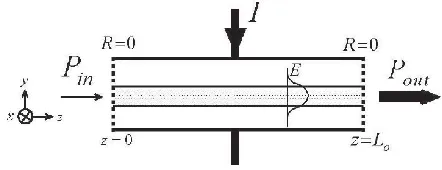
Figure 1 Structure of semiconductor optical amplifier (SOA)
Structure of semiconductor optical amplifier (SOA) used in this analysis is shown in Figure 1. The front and back facets of the SOA are anti-reflection coated to prevent reflections. The length of SOA is Lo, the width
and thickness of the active region are w and d, respectively. The signal wave propagates in the z -direction. The driving current is I and the input power of the signal is
P
in.For this analysis, we introduce two types of electric polarization into the classical Maxwell’s wave equation,
0
E
sp, (1) where χ is the laser susceptibility giving the stimulated emission (amplification)and Psp is anotherpolarization giving the spontaneous emission. Then, the Maxwell’s wave equation is given as
2 2 0 0
2 2 0 0 2 2 0 2
t P
t E t
E t
E
E sp
.(2) The electric field component Eis given with ()
E
and ()
E as the forward and the backward
propagating optical waves to be
) ( ) (
E E
E , (3)
where
. . )
, ( ) , (
) (
c c e
y x z t A
E j z j t
m m
m
m
, (4)
. . )
, ( ) , (
) (
c c e
y x z t B
E j z j t
m m
m
m
. (5)
Here, m is the longitudinal mode number which cover all modes including the signal mode and the ASE modes,
(x,y) is normalized field distributionfunction in the transverse cross- section, ωmis angular
frequency, βm is propagation constant and c.c.
backward propagating waves of the mode m, respectively.
Although we are investigating properties of the forward propagating wave in the SOA, we need to take into account existence of the backward propagating wave, because the spontaneous emission generates in both the forward and the backward direction simultaneously. In this paper, we adopt three improvements from our previous published papers in refs. [14, 16]. This additional count of the backward propagating wave is the first improvement.
2.2 Photon and Longitudinal Modes
The spontaneous emission is caused by the zero point energy of the quantized optical field [17]. We define the photon and longitudinal modes for the ASE as followings: We suppose a finite length
L
f with whichthe photon number is defined. The optical energy W
in the supposed length
L
fis given as
m
m m
m L z
L z
S
S
dz
dy
dx
E
E
W
ff
2
1
) ( ) ( 2 / 2 /
2 ) ( 2 ) (
. (6)
Here, ()
m
S
and ()m
S
are photon numbers of theforward and backward propagating optical wave of mode m, respectively. The zero-point energy of the quantized optical wave
(
1
/
2
)
mis originally definedwith a standing wave, which is a superposed mode of the forward and the backward waves, and should be uniquely defined with the quantum number 1/2 without doubling the quantum number. Other zero-point energy at same spatial position must be belong to different longitudinal modes.
Then, we can define longitudinal mode m with condition of
mL
f2
m
2
. (7) Orthogonal relations among the signal mode and all ASE modes are guaranteed. The propagation constant is characterized with equivalent dielectric constant or equivalent refractive index 2eq
n
o eq
,and propagation speed v and optical frequency
f
moas in the followings :
v
f
mo meq m
0
2
, (8)eq n
c
v . (9)
Figure 1 Introduction of finite length
L
fto define longitudinal modeOur idea for introduction of finite length
L
fisillustrated in Figure 2. Criterions on the supposed length
L
fwill be given in Subsection 2.4.Although discrete values of the mode number m are supposed, the output ASE profile reveals continuous spectrum as shown in Figure 3 because of the spectrum broadening by each ASE mode. Figure 3 is a calculated example based on our proposed model. The center peak is the signal mode, fine Lorentzian shape spectrum show contribution from each ASE mode and flat spectrum is summed up output of the ASE modes. Calculation manner is given in Sections 3 and 4.
Figure 2 An example calculated of light output spectrum from an SOA
2.3 Gain and Spontaneous Emission
The amplitude
A
m(
t
,
z
)
is factorized to an absolute value and phase term:) , (
) , ( ) .
( m j tz
m
m
e z t A z t
A , (10)
where θm (t,z) is the optical phase
The carrying optical power Pm(t,z) of the forward
f m m
m eq m
m m
L v S
z t A n
dy dx H E z
t P
) (
2 0
0 )
( ) (
) , ( 2
) , (
[W].
(11)
where ()
m
E
and ()m
H
are electric and magneticcomponents of the mode m, respectively.
Dynamic equation of optical power Pm(t,z) is
obtained from Maxwell’s wave equation given in equation (2) with suitable manipulation and quantum mechanical modification [14]:
) , ( )
( 1
z t F L L
vg P
g t P v z P
m f
m f
em m m m m
m
,
(12) where gm is the gain coefficient, κ is the guiding loss
coefficient and Fm is the Langevin noise source for
photon number. Note that em
vg
indicates thespontaneous emission.
In this paper, we take up an SOA which is made of InGaAsP system having a quantum well structure. Then, the gain coefficient gm shows saturation
phenomena with increasing of electron density n. We propose here an approximated expression of the gain coefficient as [16].
bn
n
n
a
g
m
g
1
)
(
, (13)
where
is the field confinement factor, a and b are the coefficient to characterize the gain coefficient.From quantum mechanical point of view, the gain coefficient gm consists of two parts,
g
emfor opticalemission and
g
am for optical absorption,corresponding to the electron transition from the conduction band to the valence band and that from the valence band to the conduction band, respectively:
am em
m
g
g
g
. (14)Then, these parts are written as
bn n a gem
1
(15)and
n b
n a
g g
am
1
(16)
2.4 Examination of Supposed Length Lf
Since the term
v
g
emgives emitting probability of thespontaneous emission, em vg
1
is a time period in which
one photon is emitted in the mode m as the spontaneous emission. During this time period, the photon propagates length
L
fwith velocity v. Afterthis time period, the next spontaneous emission is generated in the mode m.
Based on discussion mentioned above, we can conclude that the supposed length
L
fmust beem em f
g
vg
v
L
1
. (17)The frequency separation of the longitudinal mode is,
2 2
) 1 (
em f mo o m m
vg L v f
f
. (18)2.5 Electron Density Variation
The three dimensional volume
V
f in the active regioncorresponding to the supposed length Lf is
f f
w
d
L
V
, (19)and total volume of the active region is
0 0
w
d
L
V
(20)The variation of electron density n in the volume Vf
is given as [14],
m m f
m m
V z t W eV
I n wd P g
dt
dn (, )
0
, (21)
where τ is the electron lifetime, e is the electron charge and W(t,z) is the Langevin noise source for the electron number fluctuation.
2.6 Optical Phase Variation
A dynamic equation for variation of the optical phase
m(
t
,
z
)
is also derived from Maxwell’s wave equation given in equation (2) with suitable quantum mechanical approximation [14]:
(
)
(
0
)
(
,
)
2
'
z
t
T
n
z
n
g
v
z
v
t
dt
d
m m
m m m
. (22)
Here, α is the linewidth enhancement factor which indicates change of the refractive index with the electron density [18].
g
m
is derivative of the gaincoefficient on the electron density defined by
n b a n g
g m
m
1
'
. (23)nis a temporally averaged (CW) value of the
electron density.
T
mz(
t
,
z
)
is a noise source giving an intrinsic phase fluctuation associating the electron transition.3.0 NOISE ANALYSIS
3.1 Frequency Expansion of Fluctuated Terms
As found from equation (22), the phase fluctuation suffers the fluctuation on the electron density nas well as the intrinsic noise source
T
m(
z
)
. The fluctuation on the electron density are determined with fluctuation on the optical intensity as shown in equations (12) and (21). Therefore, we need to analyze fluctuations on all temporally changing variables to determine the FM noise.We expand the noise sources with noise frequency components;
F z e d z
t
F j t zv
m m ) ( ) ( ) ,
( , (24)
W z e d z
t
W(, ) ( ) j (t zv) . (25)
T z e d z
t
T j t zv
m m ) ( ) ( ) ,
( . (26)
Here,
N
f
2
(27)is an angular frequency corresponding to the noise frequency
f
N.In this paper, we expands the temporally changing variables with
exp[
j
(
t
z
/
v
)]
not with]
exp[
j
t
, although we usedexp
[
j
t
]
in [14, 16], because the fluctuations should propagate with velocity v same as the optical field in the SOA. Expansion withexp[
j
(
t
z
/
v
)]
must be suitable to represent the traveling wave, andexp[
j
t
]
is suitable for the standing wave. This replacing is the second improvement from our previous analyses in [14, 16].Then the optical power, electron density and gain coefficients are represented with continuous wave (CW) terms and fluctuating terms as follows:
z e d
P z P z t
P j t zv
m m m ) ( ) ( ) ( ) ,
( . (28)
n z n z e d z
t
n(, ) ( ) ( ) j (t zv) , (29)
z e d
n g z g z t
g j t zv
m m m ) ( ) ( ) ( ) ,
( , (30)
ze d
n g z g z t
g j t zv
m em em ) ( ) ( ) ( ) ,
( . (31)
3.1 Propagation of Intensity Noise
By substitution of equations (24), (28) – (31) into equation (12), we get equations for spatial variations of the CW term and the fluctuating term of the optical power along z-direction respectively as:
emf m m m m
g
L
v
P
g
z
P
, (32)
m f m m f m m m m mF
L
n
g
L
v
P
P
g
z
P
.(33) We also substitute equations (25), (28) - (30) into equation (21) and obtain equations for the CW term and the fluctuating term of the electron density respectively as:
m m m m eV I n wd P g 0 0
, (34)
m m m m m m m m fwd
P
g
j
wd
P
g
V
W
n
1
. (35)
Substitution of equation (35) to equation (33) gives,
m f m p p p p p p p p f m f m m m m mF
L
wd
P
g
j
wd
P
g
V
W
g
L
v
P
P
g
z
P
1
, (36)
Now, we derive an equation for auto-correlated value of the intensity fluctuation, because amount of the fluctuation are evaluated with auto-correlated value. From equation (36), we get
F P L wd P g j W P V L v P g P wd wd P g wd P g L v P g g g z P P P z P z P m f m p p p m m f f m m m m m p p p m p p p m f m m m m m m m m m m Re 2 1 Re 2 1 1 2 ' ' 2 2 ' 2 ' ' * * 2
, (37) Although the auto-correlated value 2
m
P is given
with a real number, the mutual correlated values
W
W
F
L
W
V
wd
z
P
g
j
L
v
P
g
W
P
wd
wd
z
P
g
j
g
L
v
P
g
W
P
g
z
W
P
m f m f p p p m f m m m p p m p p p m m f m m m m m m
2 ' ' '1
)
(
1
)
(
, (38) 2 ' ' 1 ) ( ' 1 ) ( '
m f m m f p p p m f m m m m p p p m f m m m m m m m F L F W V wd P g j L v P g wd wd P g j L v P g g g z F P
. (39) Here, we have supposed that
W
/
z
andz
F
m
/
are very small as a first order approximation.Auto-correlated value of the carrier density fluctuation is given from equation (35) as
2 ' 2 2 2 2 2 2 1 Re 2 m m m m f m m m m f m m m m f wd P g V P g L W P wd g L W n
. (40) The correlated values of Langevin noise sources are given with CW components of the electron density and the optical power as:
em m f m am em
m
L
P
v
g
g
g
F
2 , (41)
m f f m f m am eme
V
I
V
n
V
P
L
g
g
W
0 2
, (42)em m f m am em m
m L P vg
g g F
W W
F
, (43)
3.2 Propagation of FM Noise
We define the shift of operating optical frequency of mode m from the original frequency
f
mo to bef
m.The shift of the frequency
f
mis derived from theoptical phase
m(
t
,
z
)
in equation (10) as,
z e d
f z f f t z
t j t zv
m m
m
m(, ) 2
2
( ) ( ) ( )
,
(44) where
m
f is temporally averaged component and
m
f
is fluctuating term. The FM noise is given by this fluctuating term as 2
m
f .
The optical phase is expressed from equation (44) to be
j
d
e
z
f
t
z
f
z
t
v z t j m m m ) ()
(
)
(
2
)
,
(
. (45)By substituting equations (26), (29), (44) and (45) to equation (22), we get an equation for spatial variation of the fluctuating term of the optical frequency as:
v
z
T
z
n
g
j
z
z
f
m m m(
)
)
(
2
2
)
(
'
. (46)
Then, variation of the auto-correlated value of
2
m
f is given as
m m m m m m m m m T f v n f g z f f f z f z f Im Im 2 * * 2
, (47)Equations for variation of Im fmn and
m m T f
Im are obtained from equation (46) as
2
4
n
g
j
z
n
f
m
m
, (48)
2
2
m m mT
v
j
z
T
f
. (49)
Here, we have assumed that
n
/
z
is very smalland are using the fact that mutual correlation between the fluctuation on the electron density
n
and the generating term
T
m is zero.From equations (48) and (49), the terms
n
f
mIm
andIm
f
mT
m are given as,'
'
(
4
)
(
)
(
Im
0 2
z mm
n
z
dz
g
z
n
z
f
, (50)
z
m m
m T z dz
v z T z f 0 2 ' ) ' ( 2 ) ( ) (
Im
. (51)Therefore, the frequency noise 2 ( ) z
fm at position z is expressed by next equation:
)
0
(
)
(
1
)
(
2
2
)
(
2 0 ' 0 2 2 2 2 2 2 2
m z z m m m mf
z
d
z
d
z
T
v
z
n
g
z
f
We find from this equation that the FM noise is proportional to square value of the noise frequency
/
2
N
f
. If the integrand variables are almostuniformly distributed along z-direction, the double integral gives
z z z z d z d
0 0
2
2
/ . Then the FM noise
of the output light is almost proportional to
2o L . Amount of the intrinsic phase noise source 2
m
T is
obtained as a divided value of the intensity noise source 2
m
F by intensity of the electric field [14]. As
discussed with equation (6) in Subsection 2.2 of this paper, the zero-point energy
(
1
/
2
)
mis originallyobtained for a standing wave which is superposed field of the forward and the backward propagating waves. Then we suppose in this paper, the zero-point energy can be shared with the forward and the backward waves by
(
1
/
4
)
m each.2 2
) (
2 2
4 1 4
4 1 4
m m f
em m f m am em
m m m
P L
g v P L g g
S F T
(53) This equation is slightly differ from similar equation in ref. [14] on the treatment of the zero-point energy. This change is the third improvement from our previous analysis in ref. [14].
3.3 Spectrum Linewidth and Measurable Spectrum
Profile
The spectrum linewidth
f
mis given with the FM noise2
m
f by putting 0 to be
2 0
4 m
m f
f
. (54) Since the FM noise is proportional to 2, the
spectrum linewidth never increase by amplification in the SOA and is fixed by the initial condition at z0.
Measuring optical spectrum is not the modal power
P
mbut a dispersed spectrum. When wesuppose the Lorentzian distribution for measuring optical frequency
f
to each longitudinal mode atmo
f
with the half linewidth
f
m, the measurableoptical power
P
(
f
)
is given by
ms m mo mm m
f
f
f
P
f
f
P
, 2
2
1
2
2
/
)
(
)
(
[W/Hz].(55) In this paper, we denote the signal mode by the input light is to be m=s and the ASE modes to be
s
m . The signal mode is a TE mode (
E
x) but the ASEmodes are generated for both TE and TM modes (
E
xand
E
y).
m,sis introduced to count this assumption.3.4 Initial Conditions
To obtain the FM noise 2
m
f and the spectrum
linewidth
f
mof the output light, we have to tracevalues of
n
(
z
)
,P
m(
z
)
, ( )2
z
n , ( )
2
z
Pm ,
) ( ) (z W z
Pm and Pm(z)Fm(z) from z0to
o
L
z
.The initial conditions at z0are,
in
s P
P (0) for ms, (56)
0 ) 0 (
m
P for ms, (57)
in
s P
P2 2
) 0
(
for ms, (58)
0 ) 0 (
2
m
P for ms , (59)
2 2
) 0
(
in
s f
f for m=s . (60)
We should be careful about the initial condition for the FM noise of the ASE mode. At the positionz0,
0
/
mz
can be supposed, but
m/
t
2
f
m isnot zero. From equation (22), the initial condition becomes
(
0
)
(
0
)
2
4
1
)
0
(
2 22 ' 2 2
mm
m
n
T
vg
f
forms(61) Since
P
m(
0
)
P
m(
0
)
0
atz0,) 0 ( 4 ) 0 (
2
em
m vg
T is obtained, which is much larger than the first term in the right side in equation (61). Then equation (61) is rewritten as
2 2
(
0
)
)
0
(
em
m
g
v
f
for ms. (62)Initial values of the linewidth are
in in
s f f
f
2
0
4 ) 0
( for ms, (63)
(
0
)
4
em(
0
)
m
g
v
f
for ms. (64)4.0 CALCULATED DATA
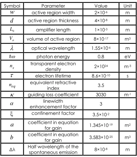
Table 1 Numerical Values of Used Parameters [14, 19]
The gain coefficient and the spontaneous emission are assumed to be identical for all modes within half wavelength
of the spontaneous emission, and those for the other modes outside of
are to be zero in order to simplify the calculation. The number of counted longitudinal modes within
is2
2
f eqL
n
M . (65)
As the operating situation, the relative intensity noise (RIN), the FM noise and the linewidth for the input signal light are assumed to be
1 15 2 2
Hz 10
/
in in in P P
RIN , 100KHz
2
in
f and
Hz 10 26 . 1
4 2 6
0
in
in f
f
thorough out this paper . A calculated example of output spectrum from the SOA has been given in Figure 3. The linewidth of the signal mode is not changed from that of the inputted signal light
f
in. Although we supposeddiscrete frequency
f
m0 for the ASE mode, obtainedASE spectrum profile becomes continuous as shown in Figure 3 because of sufficiently large value of
)
0
(
m
f
.As given in equation (52), main valuables to decide the FM noise are the electron density fluctuation 2
n and the intrinsic phase fluctuation
2
m
T . These values are changed with the CW
components of the electron density and the optical power.
Variation of the electron density
n
(
z
)
along propagating distance z is shown in Figure 4. Whenthe input signal power
P
in exceeds 1 mW, saturationor reduction of the electron density becomes large.
Figure 3 Variation of electron density along propagation
Figure 4 Frequency dispersion of the FM Noise
Frequency dispersion of the FM noise of output signal light f2(L0)
s is shown in Figure 5. As found from equation (52), the FM noise added in the SOA is proportional to 2, the FM noise hardly increase in
the lower frequency region, but rapidly increase in the high frequency region.
Figure 5 Electron Density Fluctuation
Symbol Parameter Value Unit
w
active region width 2×10⁻⁶ md
active region thickness 4×10⁻⁸ m0
L amplifier length 1×10⁻³ m
o
V volume of active region 8×10-17 m3
optical wavelength 1.55×10⁻⁶ m
photon energy 0.8 eV
g
n transparent electron
density 2×1024 m-3
electron lifetime 8.6×10⁻¹⁰ seq
n equivalent refractive
index 3.5
guiding loss coefficient 3030 m-1
enhancement factor linewidth 3
confinement factor 3.5×10⁻²a
coefficient in equation for gain 1.345×10⁻¹⁹ m2b
coefficient in equation for gain 3.583×10⁻²⁵ m3Figure 7 Intrinsic Phase Fluctuation
Variations of the carrier density fluctuation
) (
2
o
L
n and the intrinsic phase fluctuation Ts (Lo
2
with the noise frequency
f
Nare shown in Figures 6and 7, respectively.
The electron density fluctuation 2( )
o
L
n reduces in higher frequency region than several 100 MHz as shown in Figure 6. On the other hand, the intrinsic phase fluctuation Ts2(Lo
keeps same value for whole frequency range as in Figure 7. Meanwhile, the FM noise increases in the higher frequency region as has been shown in Figure 5. These facts mean that the higher FM noise in the higher frequency region comes only from the intrinsic phase fluctuation
o s L
T2(
.
The effect of the linewidth enhancement factor on the FM noise is examined as shown in Figure 8 by changing value of the linewidth enhancement factor. We find that the linewidth enhancement factor scarcely affects on the FM noise characteristic, because the FM noise in the low frequency region is low enough and that in the high frequency region does not suffer the electron density fluctuation.
Since we define the longitudinal modes for both the inputted signal mode and the ASE modes holding the orthogonal relations, there is no direct interaction among these modes. Possibility to induce interaction among these modes is through the electron density fluctuation 2
n which is caused by all existing
modes. However, the effect from the electron density fluctuation on the FM noise is very weak. Then, we can conclude that the ASE does not affect on the FM noise of the inputted optical signal.
Figure 6 FM Noise with several linewidth enhancement factor
From equation (53), we find that the intrinsic phase fluctuation 2
s
T of the signal mode becomes smaller
by increasing the optical power
P
s. Then the FMnoise given in Figure 5 shows the smaller value for the higher input optical power
P
in.5.0 EXPERIMENTAL VERIFICATION
The setup used for the experimental measurements is illustrated in Figure 9. The FM noise was measured using an interferometer and evaluated electrically through a photodetector (PD) similar with refs. [20, 21].
Figure 9 Setup used for experimental measurements
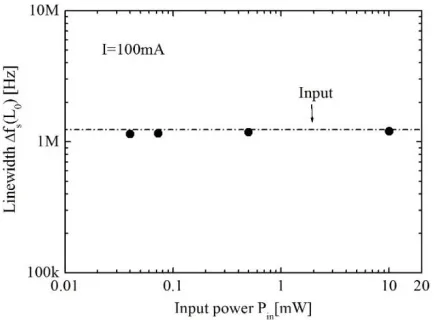
Figure 11 Experimentally measured values for the linewidth. The linewidth of the output light hardly change from that of the input light
We measured the FM noise of the DFB laser (LD) used as the source of the input light for the SOA. The LD oscillation wavelength was 1545.6nm, the driving current was 150mA and output power from LD was 23.7mW. The output power was adjusted to be 10mW by an optical attenuator (ATT).
We inserted the SOA by connecting it to the ATT and measured the FM noise of the output light from the SOA. The FM noise level of the input light was fixed by setting the injection current of the LD to be 100 KHz, while the input power of the SOA was adjusted by the ATT. The driving current of the SOA was I=100mA.
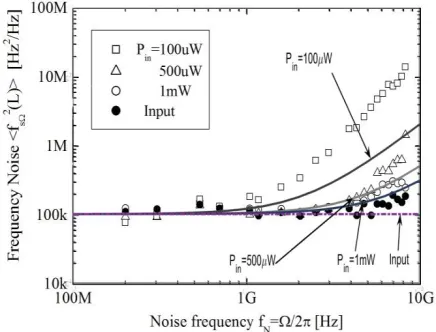
Experimentaly measured and theoretically calculated FM noise spectrum are shown in Figure 10. We found that the characteristics of frequency dependence of the FM noise of output light can be well explained by our theoretical analysis. Slight diffences between the experimental data and theoretical analysis may come from insufficient selection of numerical parameters given in Table 1.
In the low frequency region, the FM noise of the output light is almost same as that of the input light. Meanwhile, the FM noise increases with the noise frequency
f
Nin the higher frequency region than1GHz especially for lower input power level.
Figure 11 shows the experimentally measured value of linewidth. The output linewidth is hardly changed from the input light. This condition is just the same with our theoretical analysis.
6.0 CONCLUSION
The characteristics of FM noise and linewidth of semiconductor optical amplifier (SOA) without facet mirrors were theoretically analyzed and experimentally confirmed. The concept of discrete longitudinal mode for the spontaneous emission was introduced as the basis of quantum mechanical characteristics, allowing the quantitative
examination of noise sources for fluctuation of the photon number, the electron density and the optical phase. The continuously broaden output spectrum profile of the amplified spontaneous emission (ASE) was well explained as a spectrum broadening of each longitudinal mode.
Obtained results by theoretical analysis are as followings:
1. The linewidth of the inputted signal light is hardly changed by optical amplification in the SOA.
2. The FM noise increases proportional to the square value of the noise frequency.
3. Fluctuation on the electron density affects on the FM noise in the low frequency region. However, effects by the electron density fluctuation is very weak because the FM noise is low enough in the low frequency region.
4. Therefore, the linewidth enhancement factor scarcely affects on the FM noise in the SOA. This results is very different property from the semiconductor laser.
5. The FM noise in the high frequency region is caused by the intrinsic phase fluctuation on the optical emission, and becomes the stronger for the lower optical power.
6. The amplified spontaneous emission hardly affects on the FM noise of the inputted signal light in the SOA.
We also experimentally confirmed the terms 1 and 2.
Acknowledgement
The authors acknowledge Dr. H. Shoji, Mr. T. Kaneko and Mr. K. Uesaka of Sumitomo Electric Industries, Ltd, for their cooperation in this study, who measured the gain coefficient and obtained several parameters of the SOA.The authors wish to thank to UTM and Ministry of Higher Education (MoHE) for the financial support through GUP/FRGS grant.
References
[1] T. Mukai and Y. Yamamoto. 1982. Noise in an AlGaAs Semiconductor Laser Amplifier. IEEE J. Quantum Electron. 18(4): 564-575.
[2] T. Saitoh and T. Mukai. 1987. 1.5μm GaInAsP Traveling-Wave Semiconductor Laser Amplifier. IEEE J. Quantum Electron. 23(6): 1010-1020.
[3] G. P. Agrawal and N. A. Olsson. 1989. Self-phase Modulation and Spectral Broadening of Optical Pulses in Semiconductor Laser Amplifiers. IEEE J. Quantum Electron. 25(11): 2297-2306.
[4] E. Berglind and O. Nilsson. 1991. Laser Linewidth Broadening Caused by a Laser Amplifier. IEEE Photon. Technol. Lett. 3(5): 442-444.
[5] S. Balsamo, F. Sartori, and I. Montrosset. 1996. Dynamic Beam Propagation Method for Flared Semiconductor Power Amplifiers. IEEE J. Sel. Top. Quantum Electron. 2: 378-384.
Saturated Semiconductor Optical Amplifier. IEEE J. Quantum Electron. 34 (3): 548-551.
[7] M. Shtaif, B. Tromborg, and G. Eeisenstein. 1998. Noise Spectra of Semiconductor Optical Amplifiers: Relation Between Semiclassical And Quantum Descriptions. IEEE J. Quantum Electron. 34(5): 869-878.
[8] M.J. Connelly. Wideband Semiconductor Optical Amplifier Steady-State Numerical Model. IEEE Journal of Quantum Electronics. 37: 3.
[9] E. Udvary, T. Banky, A. Hilt and T. Marozsak. 2003. Noise and Gain Properties of Semiconductor Optical Amplifier. In proceeding of IEEE Transparent Optical Network Conference, 2003.
[10] A. Champagne, J. Camel, R. Maciejko, K. J. Kasunic, D. M. Adams, and B. Tromborg. 2002. Linewidth Broadening in a
Distributed Feedback Laser Integrated with a
Semiconductor Optical Amplifier. IEEE J. Quantum Electron. 38(11): 1493-1502.
[11] G. Morthier and B. Meyersoon. 2002. Intensity Noise and Line Width of Laser Diodes with Integrated Semiconductor Optical Amplifier. IEEE Photon. Technol. Lett. 14(12): 1644-1646.
[12] A. Bilenca and G. Eisenstein. 2005. Statistical Noise Properties of an Optical Pulse Propagating in a Nonlinear Semiconductor Optical Amplifier. IEEE J. Quantum Electron. 41(1): 36-44.
[13] X. Wei and L. Zhang. 2005. Analysis of the Phase Noise in Saturated Soas for DPSK Applications. IEEE J. Quantum Electronics. 41(4): 554-561.
[14] M. Yamada. 2012. Analysis of Intensity and Frequency Noises in Semiconductor Optical Amplifier. IEEE J. Quantum Electron. 48(8): 980-990.
[15] M. Yamada, N. Takeuchi, K. Sakumoto, and Y. Kuwamura. 2012. Variation of Relative Intensity Noise with Optical Power in InGaAsP Semiconductor Optical Amplifier. IEEE Photon. Technol. Lett. 24(22): 2049-2051.
[16] K. Higuchi, N. Takeuchi, and M. Yamada. 2014. Peculiar Characteristics of Amplification and Noise for Intensity Modulated Light in Semiconductor Optical Amplifier. IEICE Trans. Electron. E97-C(11): 1093-1103.
[17] M. Yamada. 2014. Theory of of Semiconductor Lasers. Springer.
[18] C. H. Henry. 1982. Theory of the Linewidth of Semiconductor Lasers. IEEE J. Quantum Electron. 18(2): 259-264.
[19] H. Shoji, T. Kaneko and K. Uesaka. Private Communication. [20] B. Daino, P. Spano, M. Tamburrini, and S. Piazzolla. Phase
Noise and Spectral Line Shape in Semiconductor Lasers. IEEE J. Quantum Electron. 19: 266-270.