Dynamic models for insect mortality due to exposure to insecticides

(1)

Dynamic Models for Insect Mortality Due to Exposure to

Insecticides

H.T. Banks,

∗

John E. Banks,

†

Sarah Lynn Joyner,

∗

John D. Stark

‡

September 4, 2007

∗_{Center for Research in Scientific Computation}

North Carolina State University Raleigh, North Carolina 27695-8205

†

Environmental Science Interdisciplinary Arts and Sciences

University of Washington Tacoma, Washington 98402-3100

‡

Department of Entomology Ecotoxicology Program Washington State University Puyallup, Washington 98371

Abstract

Ordinary differential equation models for insecticide induced sublethal damage and delayed death in insect populations are considered. It is shown that such models with time varying mortality rates provide excellent fits to experimental data for populations subjected to numerous levels of insecticide exposure. The effects on fecundity rates are also examined.

Key words: Differential equation models, insect populations, insecticide exposure, time varying mortality

rates

1 Introduction

(2)

2 Experimental Procedure and Data Description

In 1995, Stark and Wennergren [10] conducted a study on the sublethal effects of the neem insecticide Margosan-O (MO) on pea aphids (A. pisum). Broad bean plants which had grown to a height of 25 cm were thinned to five per pot, and the upper and under surfaces of the leaves of the plants in each pot were sprayed with water (control) or one of six concentrations ofMO. Effects ofMOon both neonate and adult pea aphids were studied in two separate procedures.

Both procedures began with two clip cages, each containing one young apterous adult female aphid, being attached to the underside of the leaves of each of the five plants in twenty-one pots for a total of ten aphids per pot. In the study of neonate exposure, three pots had been treated per concentration ofMOor water, for a total of 30 aphids per concentration. Twenty-four hours after introduction of the adult aphids, all aphids except one first instar were removed from each clip cage in order to ensure that only newborn aphids, exposed at birth to the treatments, would be observed. Mortality and reproduction data were taken daily throughout the lifespan of these newborn aphids.

Time measurements were recorded in terms of age classes whose duration was one day, beginning with age class zero. Mortality data was recorded as the number of the original 30 aphids alive each day, and reproduction data was recorded as the number of new aphids born per day. No data was recorded for these newborn aphids other than the number born; after being counted, these first instars were removed from the clip cages, leaving only the original population of aphids that had been exposed to the treatments.

In the study of adult exposure, all of the plants in each of the twenty-one pots were treated with water, and twenty-four hours after introduction of the adult aphids, all aphids except one first instar were removed from the cages. One day after these aphids had molted to the adult stage (i.e., aphids were now 7 days old), a separate set of broad bean plants was treated with either water or one of the six concentrations ofMOas described above. After the leaves had dried, the aphids were transferred to the treated plants and contained in new clip cages, with a total of 30 aphids per concentration. Mortality and reproduction were recorded daily throughout the lifespan of these aphids in the same manner as for the neonates. For a more detailed explanation of the experimental procedure, see [10].

3 Necessity of Time-Varying Parameters

The use of time-dependent parameters with this data was first considered in the context of a widely used partial differential equation model [1, 2]. The Sinko-Streifer [7] or McKendrick-von Forester [5] model for age- or size-structured population dynamics was used as a continuous-time approximation to the mortality data. This model can be expressed as

∂u

∂t +

∂

∂xgu=−µu (1)

wherex∈(x0, xmax) andt∈(0, T) with the boundary condition

R(t) =g(x0, t)u(x0, t) =

Z xmax

x0

k(x, t)u(x, t)dx

and initial condition

u(x,0) =φ(x).

Here,u(x, t) represents the population density at agexand timet,g(x, t) is the individual growth rate,φ(x) is the initial age distribution,krepresents the fecundity rate, and µis the mortality rate.

The mortality rate µ was first considered as a constant and was estimated using an ordinary least squares technique to find the parameter value that optimized the fit between the data and the model. Next, the mortality rate was taken to be time-dependent and was estimated as a piecewise constant function

µ =µ(t)≈ µM₍_t_{) =} PM

j=1ajχj(t). The ordinary least squares (OLS) technique was applied in this case

(3)

was performed to determine whether increasing the number of nodes significantly improved the fit of the model to the data [3]. It was determined that using any more than M = 5 nodal points did not result in a statistically significant improvement in the model fit when using model (1) with piecewise constant time varyingµ.

Finally, a comparison was made between the fit to the data of the Sinko-Streifer models with constant mortality and time-varying mortality, respectively. The time-varying mortality model generated a good fit to the data, capturing the aphid decline over the entire duration of the experiment, whereas the constant mortality model overestimated the population decline across the entire range of pesticide concentrations, particularly within the first 15 days. This comparison reveals the potential merits of using time-varying parameters in modeling population trajectories of organisms subjected to pesticides: the constant-parameter version of the model requires that the mortality rate be fixed at the outset, while the time-varying parameter model allows for changing mortality rates due to the cumulative effects of the toxicant.

In this note we investigate the importance of using partial differential equations (with size/age structure) such as (1) with data sets such as that described above and in [1, 10]. More precisely, we shall show that simpler ordinary differential equation (ODE) models with time varying mortality rates provide excellent fits to the data at all exposure levels. These models are much easier to formulate and use than partial differential equations such as (1) as used in [1, 2] and provide equally good descriptions/fits of the experimental data and underlying growth/mortality phenomena.

4 Development of an ODE Model

4.1 Different Mortality Types

The desire to understand the mechanisms underlying the population dynamics resulting from the toxicological insult motivates another approach to modeling the action of the insecticide. The application of MO has several effects on aphids, including both acute and sublethal toxicity. First, Neem oil combined with the surfactant that facilitates adherence of the insecticide to the plants’ leaves can coat an aphid’s exoskeleton upon contact, causing the aphid to suffocate immediately. Second,MO inhibits insect growth by acting as a molt hormone regulator. Juvenile insects exposed to the insecticide may fail to molt or may molt improperly, resulting in delayed death. Finally, exposure of adult insects toMO can reduce egg production, a sublethal effect on population growth over time.

The Sinko-Streifer model with time-varying mortality provided a highly accurate fit to the data due to its ability to capture changing mortality rates over time. However, the aphid-pesticide system can be modeled with a simple ordinary differential equation if the effects of the pesticide are ascribed to accumulation through time rather than as specific to each age class.

To reflect the modes of action of the pesticide, the time-varying mortality used in the Sinko-Streifer model was refined by partitioning it into three separate mortality rates: mortality due to the direct or immediate action of the pesticide, denotedpdir, and the delayed, cumulative effect of the insecticide,pdelay. Finally, the

functionµ(t) models the background or natural mortality experienced by all aphids. The ODE that models the population dynamics is a function of these three types of mortality and can be written

˙

x(t) =−[pdir(t) +pdelay(t) +µ(t)]x(t). (2)

(4)

4.2 Numerical Techniques

Each mortality rate is taken as a function of time measured in days, and these three functions are approxi-mated using piecewise linear splines. Each rate function has the form

q(t) =

n

X

j=0

αjℓj(t), j= 0,1, . . . , n, (3)

where n is the number of intervals into which the time span is partitioned, the αj are constants (nodal

values), andℓj is the linear spline function defined as

ℓj(t) =



   

   

t−tj−1

tj−tj−1

ift∈[tj−1, tj],

tj+1−t

tj+1−tj ift∈[tj, tj+1],

0 otherwise.

(4)

The support for µ(t) is taken as the entire time span [0, T], while the supports forpdir(t) and pdelay(t)

are restricted to smaller intervals. These intervals differ between the neonates and the adults due to the differing exposure times and to the molt regulatory action of the Neem insecticide. We take uniform 1-day discretizations {tj} on each support region so that [tj−1, tj] corresponds to one day for all piecewise linear

time dependent parameters.

Neonate aphids become adults between ages 5 and 7 days, and they undergo several molts until they have reached this stage. Molting no longer occurs for adult aphids, so the only direct effect is suffocation, which takes place over a shorter time period than does the molting. Additionally, the neonates are exposed to the insecticide at time t = 0, while the adults are exposed at timet = 7. Thus the support for pN

dir(t),

the immediate mortality for neonates, is the interval [0,6], while the support ofpA

dir(t) for immediate adult

mortality is the interval [7,9]. These intervals are partitioned so that there is one node at each discrete time tj, and in each case the rate function is constrained so that the value at the final endpoint is zero.

Thus there are a total of 7 nodes and hence 6 nontrivial coefficientsαN

j for the neonates and 3 nodes with 2

corresponding nontrivial coefficientsαA

j for the adults.

Support forpdelay(t) for both neonates and adults begins at the last node of the support forpdir(t) and

continues through the end of the time span for the data, again with the intervals partitioned such that nodes are taken daily. Here no constraints are imposed upon the spline coefficient values at the ends of the interval.

5 Parameter Estimation

A separate set of parametersθ= (α0, α1, . . . , αn) was estimated for each insecticide exposure level for both

neonate and adult aphids. This parameter estimation was performed using the ordinary least squares (OLS) inverse problem technique, where values ofθ are sought to provide the most accurate fit of the population dynamics to the data. This was carried out using a minimization of the least squares cost functional

J(θ) =

n

X

j=0

xmod(tj;θ)−xdj

2

, (5)

where xmod(tj;θ) is the solution of the model ordinary differential equation (2) at time tj for a given set

of parameters θ, and xd_j is the experimental data at timetj. The MATLAB optimization routine fmincon

(5)

5.1 Estimating Natural Mortality

The natural or background mortalityµ(t) for aphids in the absence of insecticide was determined using the OLS technique for (2) withpdir(t) =pdelay(t)≡0, which simplifies to

˙

x(t) =−µ(t)x(t) (6)

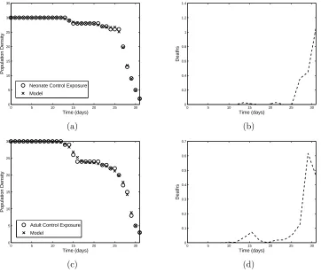
in the control situation. Since separate control data was given for each of the two age groups, a set of parameters {βi}16i=0 was estimated for each natural mortality function µN(t) and µA(t) for neonates and

adults, respectively. The results (model solutions and parameters) from these calculations are plotted in Figure 1. The small residuals seen in Table 1 confirm the qualitative observation that the model provides a highly accurate fit to the data. It can also be observed that the plot of the estimated natural mortality

µ(t) behaves as expected for both age groups: the death rate is low throughout the time span until the last three to five days, when the rate increases sharply, indicating the natural limit of the aphids’ lifespan is approaching.

5.2 Estimated Mortality Due to Insecticide

Using the estimated parameters forµ(t) in (2), the OLS technique was employed again to find parameters for pdir(t) and pdelay(t) which provide the most accurate fit to the population dynamics for populations

subjected to insecticide exposure. The parameter estimation was performed for each level of exposure for

0 5 10 15 20 25 30 0

5 10 15 20 25 30 35

Time (days)

Population Density

Neonate Control Exposure

Model

0 5 10 15 20 25 30 0

0.2 0.4 0.6 0.8 1 1.2 1.4

Time (days)

Deaths

(a) (b)

0 5 10 15 20 25 30 0

5 10 15 20 25 30

Time (days)

Population Density

Adult Control Exposure

Model

0 5 10 15 20 25 30 0

0.1 0.2 0.3 0.4 0.5 0.6 0.7

Time (days)

Deaths

(c) (d)

(6)

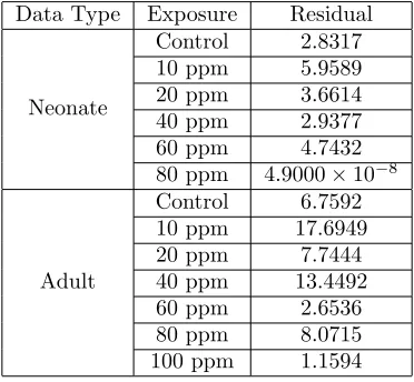
Table 1: Summary of least squares residuals for ODE model fit to pea aphid data for exposure toMO.

Data Type Exposure Residual

Neonate

Control 2.8317 10 ppm 5.9589 20 ppm 3.6614 40 ppm 2.9377 60 ppm 4.7432 80 ppm 4.9000×10−8

Adult

Control 6.7592 10 ppm 17.6949 20 ppm 7.7444 40 ppm 13.4492 60 ppm 2.6536 80 ppm 8.0715 100 ppm 1.1594

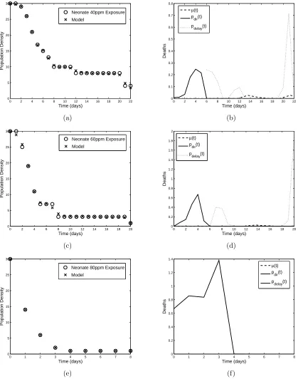
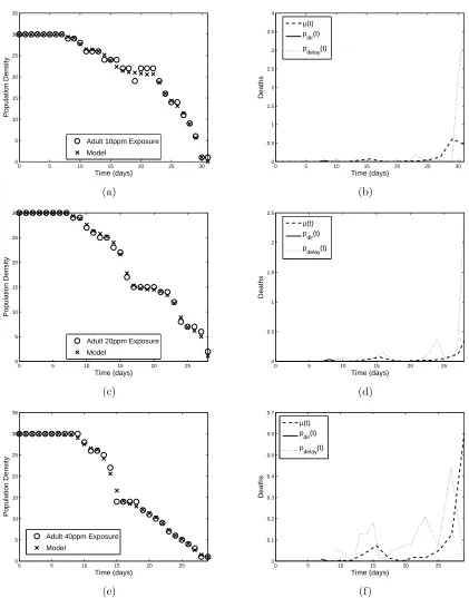
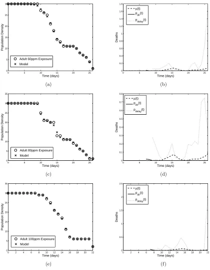
both neonates and adults, and the results are shown in Figures 2-5, with the minimized residuals summarized in Table 1.

The different modes of action of the insecticide are shown clearly in the results of the parameter esti-mation. For example, Figures 2(b) and (d) and 3(b),(d), and (f) depictpN

dir(t) increasing with insecticide

concentration, while Figures 4 and 5 reveal thatpA

dir(t) is almost negligible. These results are consistent with

the fact that the growth hormone regulatory effects play an important role in the action ofMO: neonates are affected strongly immediately after exposure, while adults have ceased molting and thus do not experience the same effects. For the adult populations,pA_delay(t) plays a more fundamental role throughout the time span as the cumulative effects of the pesticide build, whilepN

delay(t) is secondary to the direct effect of the insecticide.

(7)

0 5 10 15 20 25 0

5 10 15 20 25 30

Time (days)

Population Density

Neonate 10ppm Exposure

Model

0 5 10 15 20 25

0 0.1 0.2 0.3 0.4 0.5 0.6 0.7 0.8 0.9

Time (days)

Deaths

µ(t) p_dir(t)

p_delay(t)

(a) (b)

0 5 10 15 20 25

0 5 10 15 20 25 30

Time (days)

Population Density

Model

0 5 10 15 20 25

0 0.2 0.4 0.6 0.8 1 1.2 1.4

Time (days)

Deaths

µ(t) p_dir(t)

p_delay(t)

(c) (d)

(8)

0 2 4 6 8 10 12 14 16 18 20 22 0

5 10 15 20 25 30

Time (days)

Population Density

Neonate 40ppm Exposure Model

0 2 4 6 8 10 12 14 16 18 20 22 0

0.1 0.2 0.3 0.4 0.5 0.6 0.7 0.8

Time (days)

Deaths

µ(t) p_dir(t)

p delay(t)

(a) (b)

0 2 4 6 8 10 12 14 16 18 20 0

5 10 15 20 25 30

Time (days)

Population Density

Neonate 60ppm Exposure Model

0 2 4 6 8 10 12 14 16 18 20 0

0.2 0.4 0.6 0.8 1 1.2 1.4 1.6 1.8 2

Time (days)

Deaths

µ(t) p_dir(t)

p delay(t)

(c) (d)

0 1 2 3 4 5 6 7 8

0 5 10 15 20 25 30

Time (days)

Population Density

Model

0 1 2 3 4 5 6 7 8

0 0.2 0.4 0.6 0.8 1 1.2 1.4

Time (days)

Deaths

µ(t) p_dir(t)

p delay(t)

(e) (f)

Figure 3: Model fit to neonate (a) 40 ppm, (c) 60 ppm, and (e) 80 ppm neem exposure data and corresponding linear spline approximations (b), (d), and (f) to pN

dir(t) and pNdelay(t) compared with previously estimated

(9)

0 5 10 15 20 25 30 0

5 10 15 20 25 30 35

Time (days)

Population Density

Adult 10ppm Exposure Model

0 5 10 15 20 25 30 0

0.5 1 1.5 2 2.5 3 3.5 4

Time (days)

Deaths

µ(t) p

dir(t)

p_delay(t)

(a) (b)

0 5 10 15 20 25

0 5 10 15 20 25 30

Time (days)

Population Density

0 5 10 15 20 25

0 0.5 1 1.5 2 2.5

Time (days)

Deaths

µ(t) p

dir(t)

p_delay(t)

(c) (d)

0 5 10 15 20 25

0 5 10 15 20 25 30 35

Time (days)

Population Density

0 5 10 15 20 25

0 0.1 0.2 0.3 0.4 0.5 0.6 0.7

Time (days)

Deaths

µ(t) p

dir(t)

p_delay(t)

(e) (f)

Figure 4: Model fit to adult (a) 10 ppm, (c) 20 ppm, and (d) 40 ppm neem exposure data and corresponding linear spline approximations (b), (d), and (f) topA

(10)

0 5 10 15 20 25 0

5 10 15 20 25 30

Time (days)

Population Density

0 5 10 15 20 25

0 0.2 0.4 0.6 0.8 1 1.2 1.4 1.6 1.8

Time (days)

Deaths

µ(t) p

dir(t)

p_delay(t)

(a) (b)

0 5 10 15 20 25

0 5 10 15 20 25 30 35

Time (days)

Population Density

Adult 80ppm Exposure

Model

0 5 10 15 20 25

0 0.1 0.2 0.3 0.4 0.5 0.6 0.7 0.8

Time (days)

Deaths

µ(t) p

dir(t)

p_delay(t)

(c) (d)

0 2 4 6 8 10 12 14 16 18 20 22 0

5 10 15 20 25 30 35

Time (days)

Population Density

Adult 100ppm Exposure

Model

0 2 4 6 8 10 12 14 16 18 20 22 0

0.5 1 1.5 2 2.5

Time (days)

Deaths

µ(t) p

dir(t)

p_delay(t)

(e) (f)

Figure 5: Model fit to adult (a) 60 ppm, (c) 80 ppm, and (e) 100 ppm neem exposure data and corresponding linear spline approximations (b), (d), and (f) topA

(11)

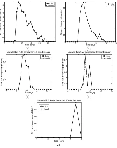
6 Effect of Neem on Aphid Fecundity

The neem insecticide also affects the fecundity of the aphids. A decrease in fecundity is expected as the concentration of the insecticide increases, and this is indeed the case, as shown in the data for the daily births, plotted in Figure 6.

The total number of births per day,R(t), can be modeled as

R(t) =r(t)x(t), (7)

where x(t) is the number of the original 30 aphids alive at time t, and r(t) is the birth rate (number of young per aphid per day). The reproduction data Rd

j is used for R(tj) with the population data xdj and

0 5 10 15 20 25 30 35

0 50 100 150 200 250

Time (days)

Births

Daily Births for Neonate Pea Aphids

Control 10 ppm 20 ppm 40 ppm 60 ppm 80 ppm

(a)

0 5 10 15 20 25 30 35

0 50 100 150 200 250 300

Time (days)

Births

Daily Births for Adult Pea Aphids

Control 10 ppm 20 ppm 40 ppm 60 ppm 80 ppm 100 ppm

(b)

(12)

0 5 10 15 20 25 30 0

1 2 3 4 5 6 7 8

Time (days)

Birth rate (new young/aphid/day)

Data Model

0 5 10 15 20 25 30

0 1 2 3 4 5 6 7 8 9

Time (days)

Data Model

(a) (b)

Figure 7: Birth rate comparison for control: (a) neonates, (b) adults.

model outputxmod(tj; ˆθγ) to compare the corresponding birth ratesrjd≡ Rd

j

xd j

withrmod(tj; ˆθγ)≡ Rd

j

xmod(tj;ˆθγ),

where ˆθγ is the optimal set of parameters determined for the insecticide exposure level γ using (5). The

resulting models rmod(tj; ˆθγ) and datardj are plotted in Figures 7 (control), 8 (neonate exposures), and 9

(adult exposures).

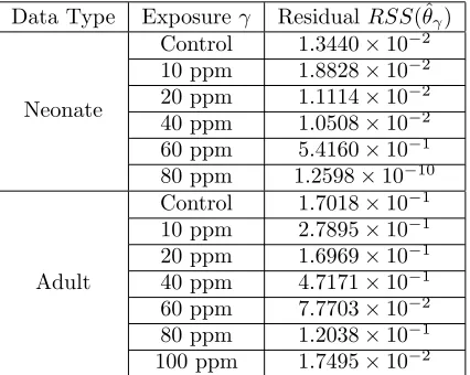
The corresponding residual sum of squares

RSS(ˆθγ) =

n

X

j=1

rmod(tj; ˆθγ)−r

d j

2

, (8)

provide a quantitative comparison of the two rates. These values are given in Table 2. Both qualitatively and quantitatively, the model output for population accurately predicts the birth rate.

Table 2: Sum of squares residuals for birth rate computed using data and model output for pea aphids exposed toMO.

Data Type Exposureγ ResidualRSS(ˆθγ)

Neonate

Control 1.3440×10−2

10 ppm 1.8828×10−2

20 ppm 1.1114×10−2

40 ppm 1.0508×10−2

60 ppm 5.4160×10−1

80 ppm 1.2598×10−10

Adult

Control 1.7018×10−1

10 ppm 2.7895×10−1

20 ppm 1.6969×10−1

40 ppm 4.7171×10−1

60 ppm 7.7703×10−2

80 ppm 1.2038×10−1

(13)

0 5 10 15 20 25 0

0.5 1 1.5 2 2.5 3 3.5 4 4.5

Time (days)

Data Model

0 5 10 15 20 25

0 0.5 1 1.5 2 2.5

Time (days)

Data Model

(a) (b)

0 5 10 15 20

0 0.5 1 1.5

Time (days)

Neonate Birth Rate Comparison: 40 ppm Exposure

Data Model

0 5 10 15 20

0 0.5 1 1.5 2 2.5 3

Time (days)

Data Model

(c) (d)

0 2 4 6 8

0 0.2 0.4 0.6 0.8 1

Time (days)

Data

Model

(e)

(14)

0 5 10 15 20 25 30 0

1 2 3 4 5 6 7 8

Time (days)

Data Model

0 5 10 15 20 25

0 1 2 3 4 5 6 7 8

Time (days)

Data Model

(a) (b)

0 5 10 15 20 25

0 1 2 3 4 5 6 7

Time (days)

Data Model

0 5 10 15 20 25

0 1 2 3 4 5 6 7

Time (days)

Data Model

(c) (d)

0 5 10 15 20 25

0 1 2 3 4 5

Time (days)

Data Model

0 5 10 15 20

0 1 2 3 4 5 6

Time (days)

Data Model

(e) (f)

(15)

7 Application to Other Insecticides

To examine the usefulness of the ODE model, another set of data for the same species was considered. Walthall and Stark examined the effects of the pesticide imidacloprid on pea aphids [11]. In this experiment, the aphids were exposed to the insecticide imidacloprid in a similar manner as in the Neem experiment. The mortality and reproduction data for all exposure levels are shown in Figure 10. Walthall and Stark observed that the aphids experienced an acute lethal response only: no sublethal effects were noted. For a more detailed explanation of the experimental procedure, see [11].

The model was adapted to correspond to these physical observations by combining the two mortality ratespdirect(t) andpdelay(t), which account for different sublethal modes of action of the insecticide, into the

one ratep(t). Thus the model is

˙

x(t) =−[p(t) +µ(t)]x(t). (9)

As before, values for the background mortalityµ(t) were found by fitting the model to the control data, and the optimalµwas used in the model to findpfor each exposure level.

As seen in Figures 11-13, this version of the model provides a good fit to the data. Since there are no sublethal effects,ptakes nonzero values that increase with the exposure level near the beginning of the time interval and values closer to zero with increasing time. These mortality rates are graphed together in Figure 14.

0 5 10 15 20 25 30 35 40 45 50

0 5 10 15 20 25 30 35 40

Time (days)

Aphids Remaining

Mortality for Neonate Pea Aphids Exposed to Imidacloprid Control 0.07 mg/L 0.1 mg/L .15 mg/L .25 mg/L .4 mg/L .6 mg/L 1.0 mg/L 1.25 mg/L

0 5 10 15 20 25 30 35 40 45 50

0 50 100 150 200 250

Time (days)

Births

Daily Births for Neonate Pea Aphids Exposed to Imidacloprid Control 0.07 mg/L 0.1 mg/L .15 mg/L .25 mg/L .4 mg/L .6 mg/L 1.0 mg/L 1.25 mg/L

(a) (b)

Figure 10: (a) Mortality for pea aphids exposed to imidacloprid; (b) Daily reproduction of pea aphids exposed to imidacloprid.

0 10 20 30

0 5 10 15 20 25 30 35 40

Time (days)

Aphids Remaining

Control Exposure Model

0 10 20 30

0 0.2 0.4 0.6 0.8 1

Time (days)

Death Rate

µ(t)

(a) (b)

(16)

0 10 20 30 40 0 5 10 15 20 25 30 35 40 Time (days) Aphids Remaining

.07 mg/L Exposure

Model

0 10 20 30 40

0 0.2 0.4 0.6 0.8 1 Time (days) Death Rate µ(t) p(t) (a) (b)

0 10 20 30 40

0 5 10 15 20 25 30 35 40 Time (days) Aphids Remaining

.1 mg/L Exposure Model

0 10 20 30 40

0 0.2 0.4 0.6 0.8 1 Time (days) Death Rate µ(t) p(t) (c) (d)

0 10 20 30 40

0 0.2 0.4 0.6 0.8 1 Time (days) Death Rate µ(t) p(t) (e) (f)

0 10 20 30 40

.25 mg/L Exposure

Model

0 10 20 30 40

0 0.2 0.4 0.6 0.8 1 Time (days) Death Rate µ(t) p(t) (g) (h)

(17)

0 5 10 15 20 25 30 0 5 10 15 20 25 30 35 40 Time (days) Aphids Remaining

.4 mg/L Exposure

Model

0 5 10 15 20 25 30

0 0.2 0.4 0.6 0.8 1 Time (days) Death Rate µ(t) p(t) (a) (b)

0 10 20 30

0 0.5 1 1.5 Time (days) Death Rate µ(t) p(t) (c) (d)

0 0.5 1 1.5 2

1.0 mg/L Exposure Model

0 0.5 1 1.5 2

0 1 2 3 4 5 Time (days) Death Rate µ(t) p(t) (e) (f)

0 0.5 1 1.5 2

0 5 10 15 20 Time (days) Aphids Remaining

1.25 mg/L Exposure

Model

0 0.5 1 1.5 2

0 1 2 3 4 5 Time (days) Death Rate µ(t) p(t) (g) (h)

(18)

0 0.5 1 1.5 2 2.5 0

0.5 1 1.5 2 2.5 3 3.5 4 4.5 5

Time (days)

Death Rate

.07 mg/L

.10 mg/L

.15 mg/L

.25 mg/L

.40 mg/L

.60 mg/L

1.0 mg/L

1.25 mg/L

5 10 15 20 25 30 35 40 45

0 0.1 0.2 0.3 0.4 0.5

Time (days)

Death Rate

.07 mg/L

.10 mg/L

.15 mg/L

.25 mg/L

.40 mg/L

.60 mg/L

1.0 mg/L

1.25 mg/L

(19)

8 Concluding Remarks

Population dynamics of one generation of aphids exposed to insecticides can be effectively modeled by an ordinary differential equation that is a function of different time-dependent mortality types, and results quantify the multiple modes of action of the insecticide. Additionally, this technique can be used to estimate population dynamics for insects exposed to pesticides with both lethal and sublethal effects. This approach may attain its highest potential when used as an alternative to static dose-response assessments of toxicity (e.g., LC50 or LD50) traditionally used in toxicological studies [8].

Although an improvement over static toxicological metrics, this model does not incorporate effects of insecticides over multiple generations, which is especially important in assessing the compatibility of pesticide use with biological control in the field [9]. A more sophisticated model (such as the age/size structured models of [1, 2]) linking generations of aphids may be needed to incorporate the sublethal effects ofMO on reproduction. A delay differential equation model that allows the population to depend on insecticide concentration and includes a maturation rate for neonates becoming adults would be a logical next step in the modeling process.

Acknowledgements

This work was supported in part (SLJ) by a CRSC/Lord Corporation Fellowship, in part (HTB and SLJ) by the US Air Force Office of Scientific Research under grant AFOSR FA9550-04-1-0220, and in part by the National Institute of Allergy and Infectious Disease under grant 9R01AI071915-05.

References

[1] H. T. Banks, J. E. Banks, L. K. Dick and J. D. Stark, Estimation of dynamic rate parameters in insect populations undergoing sublethal exposure to pesticides, Bulletin of Math Biology, DOI: 10.1007/s11538-007-9207-z, to appear.

[2] J. E. Banks, L. K. Dick, H. T. Banks and J. D. Stark, Time-varying vital rates in eco-toxicology: selective pesticides and aphid population dynamics, Ecological Modelling, DOI: 10.1016/j.ecolmodel.2007.07.022, (2007) to appear.

[3] H. T. Banks and K. Kunisch,Estimation Techniques for Distributed Parameter Systems, Birkhauser, Boston, 1989.

[4] H. Caswell,Matrix Population Models, Sinauer Associates, Inc. Publishers, Sunderland, Massachusetts, 2001.

[5] Mark Kot,Elements of Mathematical Ecology, Cambridge University Press, Cambridge, 2001.

[6] National Research Council,The Future Role of Pesticides in US Agriculture,National Academy Press, Washington, D.C., 2000.

[7] J. W. Sinko and W. Streifer, A new model for age-size structure of a population,Ecology, 46(1967), 910–918.

[8] J. D. Stark and J. E. Banks, Population-level effects of pesticides and other toxicants on arthropods, Annual Review of Entomology,48(2003), 505–519.

[9] J. D. Stark, R. Vargas and J.E. Banks,Incorporating ecologically relevant measures of pesticide effect for estimating the compatibility of pesticides and biocontrol agents,Journal of Economic Entomology

(20)

[10] J. D. Stark and U. Wennergren, Can population effects of pesticides be predicted from demographic toxicological studies? Journal of Economic Entomology,88(1995), 1089–1096.