University of Windsor University of Windsor
Scholarship at UWindsor
Scholarship at UWindsor
Electronic Theses and Dissertations Theses, Dissertations, and Major Papers
2014
Web Service Network Analysis
Web Service Network Analysis
Avani Gade
University of Windsor
Follow this and additional works at: https://scholar.uwindsor.ca/etd
Recommended Citation Recommended Citation
Gade, Avani, "Web Service Network Analysis" (2014). Electronic Theses and Dissertations. 5139. https://scholar.uwindsor.ca/etd/5139
This online database contains the full-text of PhD dissertations and Masters’ theses of University of Windsor students from 1954 forward. These documents are made available for personal study and research purposes only, in accordance with the Canadian Copyright Act and the Creative Commons license—CC BY-NC-ND (Attribution, Non-Commercial, No Derivative Works). Under this license, works must always be attributed to the copyright holder (original author), cannot be used for any commercial purposes, and may not be altered. Any other use would require the permission of the copyright holder. Students may inquire about withdrawing their dissertation and/or thesis from this database. For additional inquiries, please contact the repository administrator via email
Web Service Network Analysis
by
Avani Gade
A Thesis
Submitted to the Faculty of Graduate Studies
through the Department of Computer Science
in Partial Fulfillment of the Requirements for
the Degree of Master of Science at the
University of Windsor.
Windsor, Ontario, Canada
2014
c
Web Service Network Analysis
by
Avani Gade
APPROVED BY
K. W. Li
Odette School of Business
S. Bandyopadhyay
School of Computer Science
J. Lu, Advisor
School of Computer Science
DECLARATION OF
ORIGINALITY
I hereby certify that I am the sole author of this thesis and that no part of this thesis has been published or submitted for publication.
I certify that, to the best of my knowledge, my thesis does not infringe upon anyone’s copyright nor violate any proprietary rights and that any ideas, tech-niques, quotations, or any other material from the work of other people included in my thesis, published or otherwise, are fully acknowledged in accordance with the standard referencing practices. Furthermore, to the extent that I have in-cluded copyrighted material that surpasses the bounds of fair dealing within the meaning of the Canada Copyright Act, I certify that I have obtained a written permission from the copyright owner(s) to include such material(s) in my thesis and have included copies of such copyright clearances to my appendix.
ABSTARCT
A Web Service is a software component that is accessible on the Web. Web Services can collaborate to form composite services, which are called Mashups. Services and Mashups interconnect with each other, forming a complex network. This technological network evolves in a large scale without central control. As a new type of software network, there is an urgent need to study its topological properties. This thesis studies the Web Service Network that consists of 4255 primitive web services and mashups collected from ProgrammableWeb.com.
DEDICATION
I dedicate this thesis to my family for their constant love and support. Epecially to my dad and mom for teaching me the importance of hardwork and higher education.
To the rest of my family for their encouragement, and to my sisters for all the trust they have in me, and their belief that I can reach my dreams.
ACKNOWLEDGEMENTS
I would like to take this opportunity to express my sincere gratitude to Dr.Jianguo Lu, my supervisor, for his steady encouragement, patience and guidance. He read numerous revisions and helped me to make some sense of the confusion, and for enlightening discussions we led through-out my graduate studies. Without his help, the work presented here could not have been possible.
I also wish to express my appreciation to Dr. Subir Bandyopadhyay, School of Computer Science, Dr. Kevin W Li, Odette School of Business and Dr. Richard Frost, School of Computer Science for being in the committee and sharing their valuable time.
Contents
Declaration iii
Abstract iv
Dedication v
Acknowledgements vi
List of Figures viii
List of Tables xi
1 Introduction 1
1.1 Web Service . . . 1
1.2 Motivation and Objective . . . 3
1.3 Problem Definition . . . 4
1.4 Thesis Contribution . . . 4
1.5 Thesis Organization . . . 4
2 Background Work 5 3 Network Centrality Measurements 11 3.1 Overview . . . 11
3.2 Visualization . . . 12
3.3 Degree Centrality . . . 14
3.3.1 Representation of Matrices . . . 14
3.3.2 Power law . . . 18
3.4 Betweenness Centrality . . . 23
3.5 Closeness Centrality . . . 28
3.6 The Average Path Length and Diameter . . . 32
3.7 Strongly and Weakly connected parts(SCC and WCC) . . . 34
3.8 Clustering Coefficient . . . 37
3.9 Ranking Web APIs . . . 38
3.10 PageRank using Damping Factor . . . 42
3.11 PageRank removing the Dead ends . . . 44
4 Correlation Between the Centralities 49 4.1 Pearson’s Correlation coefficient . . . 49
4.2 Top Nodes . . . 51
4.4 Summary of Power law distribution in software . . . 55
5 Conclusion and Future Work 56
Bibliography 61
List of Figures
1.1 An Example Web Service Network . . . 2
2.1 A Sample Class Graph . . . 5
2.2 Validating the small world from Log-log plot of the class graph . . . 6
2.3 A simple class collaboration graph representing the relationship among the classes A, B, C, D. . . 7
2.4 An example of Component Graph . . . 8
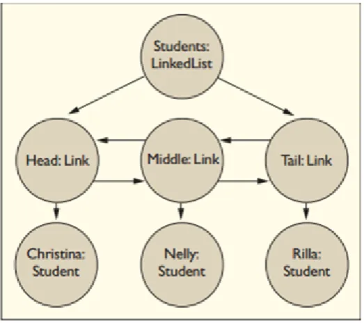
2.5 A simple object graph of a Linked List . . . 9
3.1 The representation of the Web Service Network . . . 13
3.2 Simple example to compute the Degree Centrality . . . 15
3.3 In-degree and Out-degree distribution for the Web Service Network 17 3.4 Degree distribution for the Web Service Network . . . 17
3.5 Power law fit to the degree distribution . . . 19
3.6 Rank plot of in-degree . . . 19
3.7 Rank plot of out-degree . . . 20
3.8 Top ten nodes with highest In-degree . . . 21
3.9 Top ten nodes with highest Out-degree . . . 22
3.10 A simple example for betweenness centrality . . . 24
3.11 Top ten nodes with highest Betweenness . . . 26
3.12 A larger example for betweenness centrality . . . 27
3.13 Table for the network . . . 27
3.14 A simple example for Closeness centrality . . . 28
3.15 Top ten nodes with highest Closeness . . . 30
3.16 A larger example for closeness centrality . . . 31
3.17 Table for the network . . . 31
3.18 An example network to calculate the diameter . . . 32
3.19 Diameter for the Web Api-Mashup Network-Undirected . . . 33
3.20 Simple example network to calculate the SCC . . . 34
3.21 Strongly connected component for the Web Api-Mashup Network . 36 3.22 An example network to calculate clustering coefficient . . . 37
3.23 An example of a network to calculate PageRank . . . 39
3.24 PageRank . . . 42
3.25 PageRank using Jump Factor 0.8 . . . 43
3.26 PageRank after removing the dead ends . . . 44
3.27 Top ten nodes with highest PageRank . . . 46
3.28 A larger example for PageRank centrality . . . 47
4.1 Logarithmic plot of Correlation between centralities for the Web Service Network . . . 50 4.2 Top 25 nodes in the Web Service Network (directed) . . . 52 4.3 Top highest score for In-degree, PageRank, Betweenness and
List of Tables
3.1 Network Centrality Measures . . . 12
3.2 Matrix for Betweenness Centrality example . . . 24
3.3 Calculating Betweenness Centrality . . . 25
3.4 Calculating the Closeness Centrality . . . 29
Chapter 1
Introduction
1.1
Web Service
The nature of the Web has expanded and changed considerably over the years. The Web that was once a repository of texts and images evolved into a provider of services. It now provides various information such as videos, news, music, shopping, flight bookings, business to business applications and many more[1]. Ten years ago the first generation Web or Web 1.0 was seen as a medium of education and communication resource, analogous to a book, as a means of representing the content or means of communicating[2]. The users browsed, read and obtained information and then were directed through a site from a front-page[3]. Web 1.0 was limited in use, seen as only people with high ability in HTML (Hypertext Mark Language) could post content.
The Web 2.0[4] collectively dubbed as new generation web-based technologies, has provided the growth of applications such as Wikis, Blogs, Social Networks, Podcasts, Mashups, etc. that make it easier for users to publish their own content unlike the unnamed Web 1.0[5][6]. Mashups are the personalized applications cre-ated by the user with the help of a programmable interface, i.e., Programmable Web[7]. The importance of these Mashups is that they can combine the content in new and suprising ways thereby creating a new webservice entirely or they can also provide a new visualisation to the already available and existing web services[8]. These Web 2.0 technologies have paved the way for the users to create their own web applications using powerful building blocks provided by third parties by enabling them to go beyond static publishing, for even more profound trans-formation. According to IanDavis[6] described that the Web 2.0 is still emerging as the Web 1.0 took people to information, whereas the Web 2.0 will take the information to the people[6].
The Web Service is defined as an application accessible to other applications over the web. Nevertheless, the definition of the Web Service to a large ex-tent depends on the underlying concepts and technologies and how it has been interpreted[10]. The UDDI (Universal Description, Discovery and Integration) consortium defines the precise definition of the Web Service as “self-contained, modular business applications that have open Internet oriented, standards-based interfaces”. This definition focuses on putting emphasis on the need for being compliant with internet standards. It also requires the service open, i.e., to have a published interface which essentially invoked across the Internet[10].
The Web Service provides the APIs. APIs are the application programming interfaces that the Mashups build on[6]. A Mashup combines data and services provided by third parties through open APIs as well as the internal sources owned by the users[11]. The Mashups are backed personally by a complex ecosystem of Mashup platforms, interconnected data providers and users[12]. The Mashups is created in a way that hides the details of the source applications to offer a seamless experience for the user by integrating data or functionality from one or more sources to create a new application[7].
The Programmable Web also categorizes the APIs and Mashups through pro-viding taxonomy and tags that users can associate with the entries. It offers information on Mashup tools, as the site is user contributed not all APIs and Mashups are indexed. However, the Programmable Web is the most widely used and recognized Mashup directory, and its content is considered the representative of the state of the Mashup ecosystem[12].
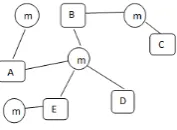
An example Web Service Network is as follows
Figure 1.1: An Example Web Service Network
1.2
Motivation and Objective
As the Web 2.0 is still evolving, no greater stability is obtained in understanding the growth of the ecosystem. Despite the development of the Web Service Net-works and its adamant features, its use is not fully known yet. The key question is how the structure of the Web Service Network looks like and how these Mashups use the APIs. According to [7] the structure of the Web Service Network is a three-tiered network with a layer of Mashups between each API tier. The inter-esting fact found is that the growth of APIs is slower compared to the growth of Mashups[7].
To understand these Web Service Networks many researchers have worked for permanence and how they evolved. However, mostly their work focused on the software architectures and other dynamic programming languages like Java, Ruby, JDK, Eclipse, etc. confining to private network as they could not be easily integrated with other languages and vice versa due to the interpretations of stan-dards, different standard versions, encodings, etc. Nevertheless, the distributed programming shifted from private to public internet and from using the private and controlled services to increasingly use publicly available Web services[13]. It is critical to understand, and there is an urgent need to study these networks. Despite many adopting the Web Service Network concept and perceiving its im-portance, it is still challenging and much effort remains before seeing the Mashup applications in a mature stage[14].
For the growth and success of the ecosystem it is critical to find the key players in the network, as they have a faster access to information and resources and to centrally transfer the information to other components. Many researchers have suggested simple rules describing the behavior of individuals in the system, leading to a unique pattern to the entire system [9]. The interaction between the entities became a significant cause of innovation and these studies initiated to use the network analysis to explore the relationship between the entities[15]. Thus, this analysis helps in designing efficient networks. Therefore, the key players in the network play an important role in the development of the network, and in the context of the Web Service Network these central nodes play an important role for the users to create their Mashups by using the influential web APIs for their success and growth.
1.3
Problem Definition
The main focus of this thesis is to analyze a new type of software network i.e., web service network and identifying the central players in the network based on the centrality to calculate the topological properties that include Degree, Betweenness, Closeness and PageRank centralities.
The aim is to also calculate the correlation between these centralities to cal-culate the linear dependency between them and how each of them is influential in the network.
1.4
Thesis Contribution
The main contribution of this thesis includes,
• To find the top Web Services based on the centralities.
• Identify if the Web Service Network follows a Power law function.
• Analyzing the Web Service Network results to see if it is a scale free network.
• Comparison between the earlier work and how it differs.
• Visual and Graphical analysis.
• To analyze the structure and layout of the Web Service Network.
• Different programming techniques with implementation using (Matlab Pro-gramming Language) to calculate the centralities and the correlation.
• The aim of this thesis is also to find if the Web Service Network is a bipartite network, which would be of great interest analyzing and drawing conclusions.
1.5
Thesis Organization
Chapter 2
Background Work
Valverde et al.[17] was the first to present a new complex network approach to software engineering based on the advances of complex networks[18, 19, 20] and the first to study the software networks. In this approach, a software network is a class graph that is a directed graph where D = (V, L) that consists of the set V of classes where every class maps to a single node in the class graph and the set of relationships in L.
Figure 2.1: A Sample Class Graph
(A) A sample UML class graph (B) Its equivalent class graph
The figure 2.1 has been produced by [17]. In this approach, the nodes represent the software entities, i.e., classes and/or methods and the edges represent the static relations between them namely the inheritance and collaboration between the classes.
They conducted experiments on a large collection of object-oriented software’s written in C++ and Java to study the scale free and small world behavior of OO software’s in many real systems and random graphs to suggest that they are the universal features of software designs. In addition, they also conducted experiments to verify if the degree distribution follows a Power law.
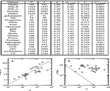
Figure 2.2: Validating the small world from Log-log plot of the class graph
(A) Average path length vs. the Class Graph size (B) Normalized Clustering followed by the random counter parts where N is the number of classes, L is the number of links, d is the average path length, drand is the average path length in random graphs, C is the Clustering Coefficient of the class graph and Crand is the Clustering Coefficient of the random graphs. The figure 2.2 is produced by [17].
Based on the above analysis they distinguished that the class graphs are much more clustered than their random counter parts and the Clustering Coefficient of the Class graphs is well above the random expectation while the average path length is rather small which proves the concept of Small world behavior. They also found the scale free behavior where a very few classes take part in various relations and the majority of classes have only one or two relationships. Even though this approach verifies the behaviors of software networks and it found universal patterns in a large collection of object-oriented softwares, it fails to take the edge direction and the centrality measurement into consideration.
author examined the collaboration networks associated with six different open-source software systems. Collaboration networks in his research refer to graphs which are decomposed into two subgraphs. Those graphs are the inheritance graph and the aggregation graph.
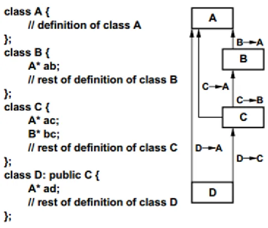
Figure 2.3: A simple class collaboration graph representing the relationship among the classes A, B, C, D.
The figure 2.3 was produced by [21]. The class collaboration in his work is defined to include the interaction of classes both through inheritance, i.e., where one class is defined as a subclass of other and through aggregation i.e., where one class is defined to hold an instance of the other class[21]. According to [21] the nodes represent the classes and the edges represent the directed collaborations between the classes.
The author conducted experiments to examine the WCC (Weakly Connected Components) and SCC (Strongly Connected Components) in his studied collabo-ration networks associated with six different open-source software systems and to verify the behaviors and features of the networks through his proposed model.
According to [21] based on his experiments concluded that all six systems consist of a single dominant WCC comprising a large fraction of the total nodes in the system and a very small remaining WCC, and conversely only few a nodes belonging to SCC. An interesting part of his work is the symmetry between the in-degree and out-in-degree which follows a Power law, concluding that the hierarchical nature of software design has an impact on the overall network topology.
view of software engineering and to uncover precise implications of that process for large-scale network.
Ichii et al.[22] proposed a new approach to explore the component graphs, i.e., statistical analysis based on OO software’s as single software systems and multiple software systems which have never been studied before. A single software systems composed of the components that are acquired by analyzing the source files which have been retrieved from the distribution packages and multiple software system is composed of the components that are acquired by analyzing the source files which have been retrieved from the distribution packages and/or software repositories. The focus of his approach is to find if the component graphs in-degree and out-degree followed the Power law.
According to [22] his research of a software component graph, referred as com-ponent graph, is a graph where the node represents the comcom-ponent and an edge represents the use relation between the components.
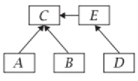
Figure 2.4: An example of Component Graph
The figure 2.4 has been produced from [22]. A component in his work refers to a Java interface or a Java class extracted from the source files and the use rela-tion represents the User Interface, that extends, implements, declares a variable, instantiated, calls, or if an interface refers to a field value of a class or an interface.
The authors conducted experiments to verify if the In-degree and Out-degree followed a Power
law[22]-• (In-degree and Out-degree of a component graph) Based on the experiment 1, the Power law is followed by the in-degree distribution almost ideally and not for the out-degree distribution and the distribution reaches highest in the range of small values while a straight line is identified in the range of larger values.
• (in-degree and out-degree distributions of a component graph for multiple software systems) Based on experiment 2, with the component graphs for multiple software systems: The the Power Law is followed by the in-degree distribution and not the out-degree distribution.
picked out based on a keyword has similar characteristic with the superset. The Power law is followed by in-degree distribution with similar parameters and the the Power law is partially followed by the out-degree distribution.
• (What aspects of components contribute to the Power Law (or non-Power Law) at the In-degree and/or Out-degree distribution of a component graph) Based on experiment 4, the In-degree relates to the roles of the components, but it has a low correlation with the size, the complexity, and the cohesion. They also found that, the out-degree has a higher correlation with the size and the complexity of the component[22].
Based on their analysis, they concluded that there was an asymmetry between the in-degree and out-degree as the in-degree followed a Power law but, not the out-degree. The authors draw conclusions that the in-degree depends on the role of each component and the out-degree depends on the size and the complexity of each component.
However, this approach failed to explain why some software’s follow the Power law and some software’s do not. It also failed to consider the topological measure-ments to find the important components in the graph.
Potanin et al.[23] examined the graphs formed by OO programs written in a variety of languages and proving them to be scale free networks. The author also proposes that his approach helps to optimize language runtime systems, improve the design of future of OO languages and re-examine innovative approaches to software design. The object graph in his work refers to the object instances created by a program and the links between them is the skeleton of the execution of that program.
The figure 2.5 has been produced from [23]. In his work, each link object has two references to other link objects, except for the head and tail of the list[23]. The node and edge represent an object, as the graph grows and changes as the program runs after every assignment statement to an object field, may create, change or remove an edge in the graph.
According to [23] conducted experiments to verify if the graphs formed by OO programs written in different languages follow the Power Law and prove to be a scale free network.
The authors claim that they have found symmetry between the in-degree and out-degree and they tend to follow a Power Law. However, they failed to take topological properties into consideration.
The above approaches are all different from each other as [17] failed to take the direction of an edge into consideration[21]. He also failed to explain certain implications in large-scale networks, and this work differs from [22] as in [21] there is symmetry between the In-degree and Out-degree, but in [22] there is no symmetry between the In-degree and Out-degree. This is caused by the difference in their definitions of the component graph particulary the difference between the use-relation as an edge[22][21]. Similarly, there is the difference between the works of [23] and [22] as in [23] component graph analyses a dynamic analysis of the software system in operation, i.e., linked list where as [21] is the static analysis of software system. Despite much work done by many authors they failed to explain why some software follows the Power law in some applications and metrics and some do not.
Chapter 3
Network Centrality
Measurements
3.1
Overview
The major companies like Google, E-Bay, Amazon, etc., have provided inter-faces to many of their services at little or no cost at all, to attract individuals or businesses to develop their composite applications with new functionalities. A well-known example of the web API is Google maps. It generates maps for a given location, and its output is integrated with other data and services into Mashups. These Mashups allow the quick creation of custom applications as they often have a short span and are created for only a specific group of users and needs [12]. Each new Mashup then attracts its own set of users additionally increasing the market reach of the API providers[24].
Summary of the Web Service Network
Nodes 4255 Edges 7193 Number of WCC 157
Number of SCC 4255 Diameter Directed Infinite Diameter Undirected 14 Average length directed Infinite Average length undirected 4.648
Max Indegree(directed) 453 Min Indegree(directed) 0 Max Outdegree(directed) 65
Min Outdegree(directed) 0 Clustering Coefficient 0
Table 3.1: Network Centrality Measures
3.2
Visualization
The ability to visualize and handle a Web service Network is very crucial. Visual-ization refers to the way of representing the structural information as diagrams of abstract graphs and networks. There are many visualization tools available today. The success depends on how the tool is selected and how the structure is displayed. Taking all these factors into consideration this thesis uses Graphviz open source graph visualization software[25]. Graphviz has various features to represent the layout of the graph the layouts include dot, neato, fdp, sfdp, twopi and circo. The layout can be selected based on the appearance of the structure of the graph. The description of the layouts is as follows[25].
• dot-In Graphviz this is a default layout. It gives the hierarchical or layered structure for directed graphs if the edges have directionality.
• neato-This layout can be used if the graph is not too large and is undirected. It uses a spring model layout and it attempts to minimize global energy function, similar to statistical multidimensional scaling[26].
• fdp-It is similar to note as the “spring model” layout. The major difference however, reduces forces rather than working with energy[27].
• sfdp-This layout may be used for larger and undirected graphs. It is a multiscale version of the fdp and produces layouts in a reasonably short time.
• twopi-It draws graphs using a radial layout[28, 29], where nodes are placed in centric circles depending on their distance from a given root node.
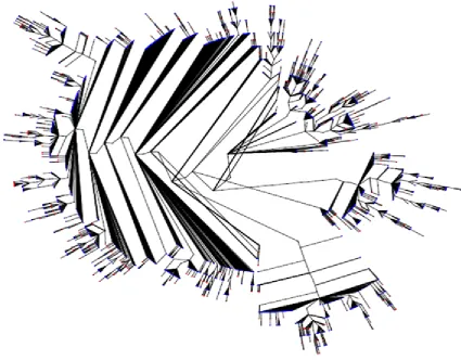
The figure 3.1 shows the Web Service Network. The red dots represent the Web API’s and the blue dots represent the mashups. The figure was produced using the Graphviz visualization tool with the twopi layout.
Figure 3.1: The representation of the Web Service Network
Finding the network centralities is an aggregate phenomenon in knowing the frequency of how the API is used in some Mashups. This way helps understand why certain APIs are vastly used and more popular than other APIs[24].
The node’s individual properties are usually expressed in terms of its centrality. The nodes that are centrally located have a more vital and important position in the network and a node has faster access to information and resources. Thus, centrality indicates the extent to which a node’s strategic position is defined by its key ties to other nodes in the network [31]. However, if a node is removed, would communication be disrupted is another problem this thesis would be focusing on.
Centrality measures indicate the importance of the Web Services in the Web Service Network. The types of centrality measurements in this research are degree centrality, betweenness, closeness and pagerank. Each of these different centrality measurements will identify the central nodes in the network based on the network position which will be examined by the measurement of each node [32].
3.3
Degree Centrality
The degree of a node is determined by the number of links or ties it has. In-degree is equal to the number of incoming edges of a node. In a network, it is natural for some key nodes to supply services to many other nodes, while most other nodes supply services only to few other nodes if any. Out-degree of a node represents a completely different property, with respect to the in-degree, it is the number of nodes used by a given node. It is merely the number of outgoing edges of a node.
According to [16] the degree distribution is the function P of a network can be calculated by fraction of the number of vertices having degree i to total number of degrees.
P(i) = N umber of vertices having a degree i
T otal number of degrees (3.1)
3.3.1
Representation of Matrices
The algorithm used to calculate the in-degree and out-degree is given in algo-rithm 1.
Algorithm 1 In-degree and Out-degree Input: Matrix
Output: In-degree and Out-degree
for all unique edges do
Matrix(Source(i, 1), Destination(i, 1))=1 In-degree=sum (Matrix)
Out-degree=sum (Matrix‘)
end for
In algorithm 1, i, represents the unique edges, the source and destination rep-resent the Web APIs and Mashups.
A simple example to compute the degree centrality is as follows.
Figure 3.2: Simple example to compute the Degree Centrality
According to [34]the degree centrality of a vertex is defined as,
di =
X
j
Aij (3.2)
Where di is the degree centrality of a vertex i, A is the adjacency matrix and Aij =1 if there is a link between node i and j,Aij =0 if there is no link.
The sum of the rows of the matrix represent the in-degree of the figure 3.2 and the sum of column represents the out-degree. The degree of the node from the adjacency matrix is the sum of the row i and column j for each node.
0 1 1 1 0 0 0 0 0 0 1 0 0 0 0 0 0 0 0 0 0 0 0 0 0 0 1 0 1 0 0 0 0 0 0 0 0 1 1 0 0 0 0 1 0 0 0 1 0 0 0 0 0 1 0 0 0 0 0 0 1 0 1 0
From figure 3.2 we can see node A has no incoming but has three outgoing edges. The in-degree of node A is 0 and out-degree is 3. The degree of node A is given by the summation of the in-degree and out-degree, i.e., 0+3=3. Similarly the degree of all the nodes can be computed. As the web API-Mashup Web Service Network is large, to calculate the topological properties this thesis uses MATLAB programming language to analyze the Web Service Network.
For analysis purpose, we first need to represent the Web Service Network in a format that allows the mathematical computation. Web Service Network in a text file format is converted to a matrix using Matlab in a way that each row and column represent the source, i.e., Web API and the destination, i.e., Mashup of the Web Service Network. And the value of row i and column j is 1 if there is a link between the source and destination or 0 otherwise. Having the matrix of the network enables us to calculate the in-degree and the out-degree by summing the corresponding column or row respectively. Once the in-degree and out-degree are calculated it is easy to find the maximum and minimum in-degree and out-degrees.
Figure 3.3: In-degree and Out-degree distribution for the Web Service Network
Figure 3.3 shows a log-log plot, the distributions of in-degree and out-degree with the base 10. The x-axis represents the degree and y-axis shows the frequency of certain degree.
Figure 3.4 gives the overall degree distribution for the Web Service Network.
Figure 3.4: Degree distribution for the Web Service Network
3.3.2
Power law
The Power law has attracted attention over the years for its mathematical and sometimes physical consequences[35]. Power law implies that small occurrences are extremely common, since large instances are extremely rare. This regularity or ’law’ is sometimes also referred to as Zipf’s law and sometimes Pareto law or the 80-20 rule i.e.; roughly 80% of the effects come from 20% of the causes [35]. According to many sources and evidences Power law distributions occur in an extremely diverse range of phenomena. They include the population of cities, sizes of earthquakes [36], moon craters [37], solar flares [38], computer files [39], the frequency of occurrence of personal names in most cultures [40], people’s annual incomes [41], the number of citations received by papers [42], the constancy of the use of words in any human language [43] and many more [16].
A network is called scale free if its degree distribution follows a Power law function. This means a high number of nodes have a small degree and only a few nodes have a high degree. This would mean that many APIs are used by few Mashups and a small number of APIs are used by many Mashups. This is the case with our Web Service Network from figure 3.3, so we can conclude that the Web Service Network follows a Power law and corresponds to a scale free network. Identifying Power laws in man-made systems or either in nature can be tricky and challenging [16].
There are many ways of generating the Power laws. A “log-log” plot provides a quick and a standard way to identify if the data exhibits an approximate Power law as it plots a straight line on log axes. But how can the Power law function be calculated is the crucial question. The best way to check if it’s approximately a Power law i1α is, for some i, estimating the exponent α.
The notion of Power law probability distribution from equation 3.1 according to [16]is expressed in the form,
P(i) = C
iα (3.3)
P(i) is the probability that i occurs, C and α are constant,α is usually expressed as the exponent. The equation 3.3 can be then expressed as,
P(i) = Ci−α (3.4)
The equation 3.4 can be expressed further by taking logarithms on both sides as,
logP(i) = −α logi+logC (3.5)
Figure 3.5: Power law fit to the degree distribution
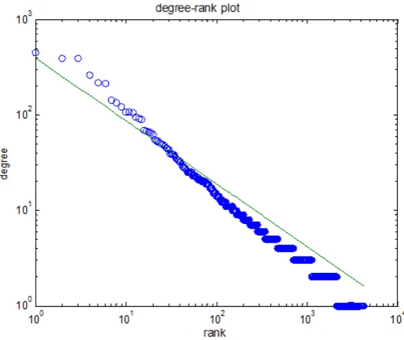
Figure 3.5 represents the Power law fit for degree distribution with an exponent
αbeing 1.66. The x-axis represents the rank, it is the decreasing order of the degree of the vertices and the y-axis represents the degree of the vertices. We can also try to fit the data of in-degree and out-degree to verify the Power law. Let us look at the plots regarding the mentioned. In the in-degree plot in figure 3.3, the tail of the in-degree seems to have a lot of noise we can try to smoothen it by plotting it on a logarithmic axis and a power law fit.
Figure 3.7: Rank plot of out-degree
The tail of the in-degree and out-degree cumulative distribution is shown in figure 3.6 and 3.7. Note how the measure on the lower right corresponds to, and whose services are used by almost every other node, and this also corresponds to a straight line. The power law fit for indegree has an expoenet of 1.66 and for out-degree is 2. If the slope of the network is high, the number of nodes having a high degree is smaller than the number of nodes having a low degree. Therefore, we can conclude that both the in-degree and out-degree follow a Power law for the Web Service Network based on the shape of the plot. The Web Service Network is also a scale free network. In the context of the Mashup ecosystem, this would imply that a large number of APIs are used by few Mashups and a small number of APIs are used by many Mashups.
Figure
3.8:
T
op
ten
no
des
with
highest
In-de
Figure
3.9:
T
op
ten
no
des
with
highest
Ou
3.4
Betweenness Centrality
The position of a Web API in a Web Service Network is characterized by the shortest path based centrality, which brings forth more information than the degree centrality . The fraction of shortest paths across a node is called Betweenness Centrality [44]. The shortest paths between each pair of nodes, and the number of times that each node appeared in the shortest paths can be computed easily. Betweenness centrality provides more topological information than rest, which is necessary in the analysis of Web Service Network. APIs with high betweenness centrality can be seen as “bridges” between clusters of APIs. The betweenness centrality is considered as an important measure for determining the control of a node on the communication between other nodes in a network[44].
For the graph G (V, E), let i and j be two nodes that are in V. The betweenness centrality for the node v ∈V according to [44] is defined as
CB(v) =
X
i6=v6=j∈V
σij(v)
σij (3.6)
whereσij is the number of shortest paths connecting i to j andσij(v) is the number
of shortest paths connecting i to j passing through the node v.
To calculate the centralities such as betweenness, closeness, diameter and av-erage path length the Web Service Network is considered, as undirected. We use the Dijakstra’s shortest path algorithm in Matlab, for the Web Service Network, to calculate the shortest path between all pairs of nodes.
Algorithm 2 Dijkstra’s Algorithm to calculate the shortest path between each pair of nodes
Input: The Web Service Network graph represented as a matrix Queue = Keeps the list of nodes to be visited
Neighbor= Keeps the list of all the neighbors for each node Output: Matrix Path and the Matrix Distance
for i=1:Number of Nodes do
distance(i,i)=0 Put i in Q=Queue
while Q is not empty do Pick a node from Q
for all neighbors of node i do
if the neighbor has not been visited before then
distance(i,neighbor(Q))=distance(i,Q)+1 path(i,neighborqueue)=Q;
add to Q=neighbor(Q);
The Matrix Path stores the path between the pairs of nodes, and Matrix dis-tance stores the length of the shortest path between each pair of nodes; and if there is no path between a pair of nodes it is equal to -1. The Algorithm 2 returns the distance and the path by calculating the shortest paths between each pair of nodes.
Let us consider a simple example to calculate the betweenness centrality.
Figure 3.10: A simple example for betweenness centrality
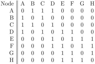
For networks like figure 3.10 it is easy to calculate the betweenness centrality of the nodes. Vertices that occur on many shortest paths between other vertices have higher betweenness than those that do not. For example, calculating the betweenness centrality for node D of figure 3.10. The matrix for figure 3.10 is as follows.
Node A B C D E F G H
A 0 1 1 1 0 0 0 0
B 1 0 1 0 0 0 0 0
C 1 1 0 1 0 0 0 0
D 1 0 1 0 1 1 0 0
E 0 0 0 1 0 1 1 1
F 0 0 0 1 1 0 1 1
G 0 0 0 0 1 1 0 1
H 0 0 0 0 1 1 1 0
For calculating the betweenness centrality let us list the number of shortest paths first. The number of shortest paths from A to E from figure 3.10 is 1. Similarly the number of shortest paths from A to F from figure 3.10 is 1 and the same follows for all other nodes. Then, we list the number of shortest paths that path through node D. For example, the number of shortest paths from A to E that pass through D is 1 and the number of shortest paths from B to E passing through D is 1 and so on. We then calculate the betweenness centrality for node D as shown in table 3.3.
Nodes σij σij(D)
σij(D)
σij
(A, B) 1 0 0
(A, C) 1 0 0
(A, E) 1 1 1
(A, F) 1 1 1
(A, G) 1 1 1
(A, H) 1 1 1
(B, C) 1 0 0
(B, E) 1 1 1
(B, F) 1 1 1
(B, G) 1 1 1
(B, H) 1 1 1
(C, E) 1 1 1
(C, F) 1 1 1
(C, G) 1 1 1
(C, H) 1 1 1
(E, F) 1 0 0
(E, G) 1 0 0
(E, H) 1 0 0
(F, G) 1 0 0
(F, H) 1 0 0
(G, H) 1 0 0
Table 3.3: Calculating Betweenness Centrality
From Table 3.3 the betweenness centrality for node D
CB(D) = 12
Figure
3.11:
T
op
ten
no
des
with
highest
Be
tw
In figure 3.11 the nodes with high betweenness centrality can be seen as ”bridges” between clusters of other nodes. An interesting observation is that nodes with high betweenness do not necessarily have a high degree.
Let us consider a simple example to verify the above case.
Figure 3.12: A larger example for betweenness centrality
Figure 3.13: Table for the network
3.5
Closeness Centrality
Between all pairs of nodes in connected graphs there is a natural distance metric, this is defined by the length of their shortest paths[45]. The farness of a node can be identified as the sum of its distances to all the other nodes, and its closeness is defined as the inverse of the farness[46][45]. If the closeness centrality of a node is 0, then its farness must be infinite in which case it is infinitely far from some node or they may be infinitely many nodes in the graph. Thus, the more dominant a node is, the lower the distance to all the other nodes. The distance between two vertices is equal to the number of edges in the shortest path connecting them. Therefore, subsequently closeness can be regarded as how fast it takes to spread the information from a node to all other nodes[47]. According to [48] closeness centrality for node v is defined as
C(v) = P 1
i∈V d(v, i)
(3.7)
where d(v,i) is the distance of the length of the shortest path between v and i and V is the set of all vertices.
As mentioned earlier, to calculate the closeness of each node the Web Service Network is considered undirected, and using algorithm 2 discussed earlier, the length of shortest paths for all pair of nodes are calculated and summed over the distance of each node to all other nodes.
An example network to calculate the Closeness centrality measure is as follows.
Figure 3.14: A simple example for Closeness centrality
Node A B C D E F G H
A 0 1 1 1 2 2 3 3
B 1 0 1 2 3 3 4 4
C 1 1 0 1 2 2 3 3
D 1 2 1 0 1 1 2 2
E 2 3 2 1 0 1 1 1
F 2 3 2 1 1 0 1 1
G 3 4 3 2 1 1 0 1
H 3 4 3 2 1 1 1 0
Table 3.4: Calculating the Closeness Centrality
The closeness for the node B and D from table 3.4 can be calculated as
CC(B) = sum of all its distances1 = 1+1+2+3+3+4+41 =181
CC(D) = sum of all its distances1 =1+2+1+1+1+2+21 =101
Nodes with high closeness centrality are noteworthy as they propagate infor-mation with more efficiency in a network in comparison with the rest of the nodes. Therefore, if we are looking to send information quickly we would start sending to the node with the highest centrality.
In the case of figure 3.14 we would first send the information to the node D. Since D can reach the rest of the network with the smallest effort. As D has a closeness of just 1/10 to reach all other nodes in the network were as B has a closeness of 1/18 to the rest of the network whereas the other nodes in the network have 13, 15 or 18.
Figure
3.15:
T
op
ten
no
d
es
with
highest
To calculate the closeness centrality we consider the nodes that have the small-est closeness unlike other as betweenness, as these nodes are close to every other node through which the flow of information can be spread to all the nodes in a small amount of time. The list of the top nodes for all these centralities is followed in Chapter 4.
Figure 3.16: A larger example for closeness centrality
Figure 3.17: Table for the network
3.6
The Average Path Length and Diameter
The average path length and diameter is based on the shortest path. The average path length is defined as the average number of steps along the shortest path for all the possible pairs of nodes in the network. The concept of average path length should not be confused with diameter. The shortest paths should be extracted among the available nodes and the longest shortest path is counted as the diameter. For a complete network, where every node is connected to every other node, the diameter of the network is 1.
Let us consider a small example to understand the concept of diameter is as follows.
Figure 3.18: An example network to calculate the diameter
For the figure 3.18 the longest shortest path is from A-H which is 4. For the directed graph, the average is taken only over the distances of those nodes that are reachable from each other and in case of those nodes that are not reachable from each other their distance is infinite. Thus, as node H cannot reach node A the longest distance is infinite. Hence the diameter of this network is infinite. If we consider the figure 3.18 as undirected every node can reach every other node.
Figure
3.19:
Diameter
for
the
W
eb
Api-Mash
up
Net
w
ork-Und
The diameter of figure 3.19 is a unique chain as length of the longest shortest path for the undirected network is 14. The nodes which appeared in the diameter are visualized in the table in figure 3.19.
3.7
Strongly and Weakly connected parts(SCC
and WCC)
A network is strongly connected if for any pair of nodes there is a path linking them. For finding the strongly connected parts of the network, it is important that we first find all the nodes that are reachable from each other. This approach enables us to find all small parts of strongly connected nodes if there is any. It is important to find strongly connected and weakly connected components to find the connectivity between the nodes and also to identify the core nodes that constitute the entire network.
Let us consider a simple example to calculate SCC.
Figure 3.20: Simple example network to calculate the SCC
Figure 3.20 can be partitioned into a unique set of strong components of SC1:(E, F, H), SC2:(G, F, H), SC3:(D). Node D is a standalone strongly con-nected componen. However, every other node cannot reach node A and node C cannot reach other nodes they are weakly connected components. Thus, the graph is a weakly connected graph.
This approach enables us to find all small parts of strongly connected nodes if there is any. The largest strongly connected part of the graph can be verified by finding the longest strongly connected part. For finding the weakly connected parts of the graph the same algorithm can be employed to the undirected graph to find the weakly connected part of the nodes if there is any. The largest strongly connected part of the graph can be checked by finding the longest strongly con-nected part.
Figure
3.21:
Strongly
con
nected
comp
onen
t
for
the
W
eb
Api-Mash
up
Net
w
3.8
Clustering Coefficient
The clustering coefficient was first introduced by Watts and Strogatz [9] in the context of social network analysis. In most real world networks, evidence sug-gests that tightly knit groups tend are created by the nodes by a relatively high density[9]. This kind of a likelihood, tends to be greater compared to the average probability of a connection randomly established between two nodes [9, 49].
The clustering coefficient measures the extent to which the network nodes tend to form groups with internal connections but few times connections leading out of the group. It is a property of a node in a network. The measure is 1 if every neighbor connected to a vertex, is also connected to every other vertex within the neighborhood and is 0 if none of the neighbors is connected. Clearly stating, clustering coefficient defined as the probability that two randomly selected neighbors are connected to each other.
According to [9] clustering coeffcient is defined as
CC(v) = Actual number of edges between neighbors of v
M aximum possible number of edges between neighbors of v
(3.8)
The actual number of edges between neighbors of v can be expressed as k(k-1)/2.
Let us consider a simple example to calculate the clustering coefficient is as follows
Figure 3.22: An example network to calculate clustering coefficient
Let figure 3.22 is a graph G. Let us consider vertex D, whose clustering coeffi-cient has to be found. The actual number of edges between neighbors of D is 2 they are (a:c,e:f). The maximum possible number of edges between neighbors of D ie., k is 4= k(k-1)/2=4(3)/2=6 . Thus clustering coeffcient of D can be expressed as
CC(D) = 2
A tree structure has no clusters by definition and the clustering coefficient of a tree is 0 [18]. For the Web Service Network the clustering coefficient is zero.
3.9
Ranking Web APIs
PageRank is considered an interesting metric to determine the relative importance of Web Services within a Web Service Network. They can be ranked in terms of ‘importance’ or ‘usefulness’ within a network so that the discovery of the solutions can be done in an effective way.
The PageRank is measured by the number of Mashups that use a particular API. Their rank again is indicated by the rank of services which use them. The algorithm for computing PageRank is provided later. For ranking the web API’s based on the Directed popularity method, each web API score is computed based on the number of its incoming-links, but all incoming-links are not equal in terms of importance, for example an incoming-link from a node that has itself a high number of incoming-links from other node has more value than an incoming-link from a node that does not have any incoming-link from the other nodes, therefore a recursive formula is required to calculate the score of each API. The Web Service APIs with higher rank have higher popularity.
According to [33] PageRank is defined as
M v =λ∗v (3.10)
M is the matrix representation of the network, v is the eigenvector of M and λ is the principal eigenvalue.
The PageRank algorithm is provided; the iteratios for the algorithm equals 20, and for each node in Matrix M if a node j has a link to i thenMij is 1/Outdegree(j)
if that element equals 1 in M otherwise 0.
Algorithm 3 PageRank
Input:Web Service Network N represented as the list of edges, Node Number(the total number of nodes)
Output: v is the rank vector containing the values M= Matrix representation of Web Service Network N
v=[1..1]/Node Number
for i=1:20 do
v=M*v
end for
v2 be v1 ∗M, v3 be v2 ∗M. The rank is converged to a fixed point as number of iterations increase. This is called the Power method. The reason for using Power method is to compute the Pagerank vector, concerns the number of iterations it requires. The converged rank i.e.,v contains PageRank values of all the nodes. The Power method is still the predominant method in finding PageRank. For the Web Service Network after a number of iterations (20) is able to calculate the rank of each node. Let us consider a simple example to calculate PageRank.
A simple example to calculate the PageRank is as follows.
Figure 3.23: An example of a network to calculate PageRank
Assume a random surfer starting at node A in figure 3.23. In order to explain what happens to the random surfers at the next step it is better to describe the matrix, if they are ‘n’ nodes, matrix M consists of ‘n’ rows and columns. If a node ’j’ has ‘k’ arcs out and if one of them is to node ’i‘ then ‘i’ is the row and ‘j’ is the column for the element M(ij) then the value is 1/k else M(ij)=0[33].
The Matrix Representation for figure 3.23 is as follows.
M=
0 1/3 1/3 1/3 0 0 0 0
0 0 1 0 0 0 0 0
0 0 0 0 0 0 0 0
0 0 1/2 0 1/2 0 0 0
0 0 0 0 0 1/2 1/2 0
0 0 0 1/2 0 0 0 1/2
0 0 0 0 0 1 0 0
0 0 0 0 1/2 0 1/2 0
A column vector can be used to best describe a random surfer’s probability. The jth component is the probability that the random surfer is at node j. This function is the PageRank[33]. Assume a random surfer starting at any of the ‘N’ nodes with a balanced probability. For each component, an initial vectorvo would
have a probability of 1/N[33]. The distribution of the surfer after one step would be
M ∗vo (3.11)
and for the next step would be
M(M vo) =M2vo (3.12)
and so on if M is the matrix. In order to know the surfers distribution after
‘i’ steps it can be found by multiplying the transition matrix M with the initial vector vo for a total of ‘i’ times[33].
A random surfers probability distribtion at node i after each step according to [33] is defined as
X
j
M(ij)∗vj (3.13)
where M(ij) is the probability that the surfer would make a move to node i in the later step being at node j and this value would be 0 as there is no link from node j to i andvj represents that the surfer was at node j at the former[33]. Given the example of this type of comportment usually relates to ancient theory called as Markov process. A surfer reaches a limiting distribution v that satisfies
v =M ∗v (3.14)
And meet the conditions:
• If it is capable of reaching from any node to every other node, i.e., if a graph is strongly connected
• If it has no dead ends, i.e., the nodes that have no arcs out
As we see the example 1 satisfies both of these above stated conditions. The distribution of M does not change by multiplying another time, rather it reaches a limit, in an alternative way the v is called as the eigenvector of M[33]. For some principal eigenvalue λ if the vector v satisfies according to [33] is defined as
then it is said to be an eigenvector for matrix M. As v has the highest eigenvalue associated to all the other eigenvalue’s it is termed as principle eigenvector and as the columns and rows of M each sum to 1 it is called a stochastic matrix. The principal eigenvalue identified with the eigenvector is 1 as M is stochastic and v is called the rank vector[33].
The position of the surfer after a long time can be known with this principle eigenvector. This intern reminds us of the intuition of PageRank i.e.: the more important a node is the more likely that a surfer will be at that node. Thus, we can start by multiplyingvothe initial vector with the Matrix M for number of rounds to see how the value differes [33]. To overcome the error limits of double precision the Web intern has 50-75 iterations for sufficient coverage [33].
Example 2: Let us see what will happen by applying the above process to matrix M. As they are five nodes, the initial vectorvo has eight components, each 1/8. The array of approximations to the limit that we get at each step by multiplying each step of M
1/8 1/8 1/8 1/8 1/8 1/8 1/8 1/8
1/8 1/8 0 1/8 1/8 1/16 1/16 1/8
1/2 0 0 1/16 1/16 1/16 1/32 3/32
1/48 0 0 1/32 3/64 3/64 1/62 3/64
1/48 0 0 1/16 7/64 3/32 3/32 1/8
and goes on
1/28 0 0 3/28 3/14 3/14 3/14 3/14
After a number of iterations the probability of A is 0.0357, the probability of B is 0, the probability of C is 0 etc. The difference of the probabilities of the nodes may not be great but in the real world situations with billions of nodes they would be greatly varying.
A similar approach of PageRanking can be applied and used for the Web Service Network. The PageRank representation for the Web Service Network is as follows.
Figure 3.24: PageRank
3.10
PageRank using Damping Factor
If there is a self loop for a node, the random surfer entering that node can never leave. Thus, all the pagerank calculated is trapped at that node. To resolve such issues the concept of teleportation came into existence. In many studies, scientists have confirmed this jump factor or the damping factor to be β and having a value of 0.8. For example consider a random surfer. The probability of a random surfer being introduced is precisely equal to that the random surfer will decide not to follow a link from their current page[33] if it has no dead ends (which will be discussed in later sections). At this point, it is clear to visualize that a random surfer decides if it has to follow the link from a current node or teleport to a random node. It is important to use the jump factor for traversing to the next nodes with the mentioned probability. Nevertheless, if a node has dead ends there is a possibility that the surfer can go nowhere.
It is simply the probability of traversing to the next nodes. Thus the prob-ability v=M*v is replaced by
v = (β∗M+ (1−β)∗R)∗v (3.16)
Where at each step we could either follow the link with the probability ofβ
Algorithm 4 PageRank using Jump Factor Input:Matrix M represented as the list of edges Output: v is the rank vector containing the values
for i=1:20 do
β=0.8
v = (β∗M+ (1−β)∗R)∗v
end for
The algorithm 4 calculates the PageRank using a jump factor 0.8. The result of applying this change is shown in figure 3.25.
Figure 3.25: PageRank using Jump Factor 0.8
3.11
PageRank removing the Dead ends
Generally, a node that has no links out is called as a dead end. By allowing the dead ends or such nodes the transition matrix can no longer be stochastic as some columns may sum to 0 instead of 1. The matrix whose columns may sum to solely 1 is called as substochastic. All the components or some of the vectors may be 0 for a stochastic matrix by computing Miv for increasing
powers. This implies that most of the important information for the network ‘drains out’ and no relative importance of the nodes is determined.
The other major problem is a spider trap. The set of nodes with no dead ends or any arcs out is called a spider trap[33]. It is because of these spider traps the pagerank calculation of a node can be trapped and the surfer cannot move any further.
If there are dead ends in the Web Service Network we replace the corre-sponding column in the matrix M with 0 and to remove the dead ends we have initially replaced them with 1/N.
Figure 3.26: PageRank after removing the dead ends
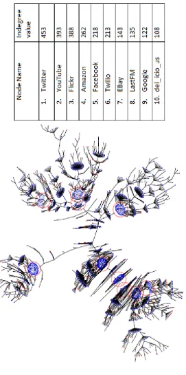
Figure
3.27:
T
op
ten
no
d
es
with
highest
P
Figure 3.27 depicts some of the nodes with the highest PageRank. The number of web services that offer an API to access their functionality has risen rapidly over the past years. Thus choosing an appropriate web service API to achieve a specific goal may be time consuming and scary for the mashup developers. PageRank is considered as an interesting metric to determine the relative importance of web services within a Web Service Network. The ranking of these Web Services serves as a heuristic guide to the success of the ranking of these web services. They can be ranked in terms of ‘importance’ or ‘usefulness’ within a network so that the discovery of the solutions can be done in an effective way.
It is not necessarily that nodes with high PageRank also have high degree, betweenness or closeness. Let us consider a simple example to verify the above scenario.
Figure 3.28: A larger example for PageRank centrality
From table 3.29 we can see that node F has a low degree, low betweenness, low closeness but has one of the highest pagerank. Observing these kind of results is really interesting to see how these nodes affect the overall network.
After PageRank was implemented a proposal called “Hubs and Authorities” was introduced. Similar to Pagerank this method also involved iterative computation of vector matrix multiplication until a fixed point. However, there are huge distinctness between these ideas, and none can be a substitute of the other. The PageRank algorithm preprocesses the steps before handling any serach queries whereas the hubs-and-authorities algorithm, was intially proposed alone for processing a search query, and to rank and produce only the responses relevant to that particular query. The Hubs and authorities may be sometimes referred to as HITS-Hyperlink Induced Topic Search[33]
Chapter 4
Correlation Between the
Centralities
4.1
Pearson’s Correlation coefficient
In order to gain access to the relation between different centralities, in this thesis we use the Pearson’s correlation coefficient. Pearson’s correlation coefficient is a measure of linear dependency between two variables. The dependence relationship between two variables can be described by using a linear function[50][51]. Pearson’s rank correlation coefficients are calculated for each pair of metrics for the Web Service Network, and the correlation between the centralities is listed in table 4.1 and are plotted in figure 4.1. The correlation between different metrics in the scatter logarithmic plot for the Web Service Network is given below.
The Pearson correlation is +1 in the case of a perfect increasing (positive) linear relationship (correlation), -1 in the case of a perfect decreasing (nega-tive) linear relationship and some value between -1 and 1 in all other cases, indicating the degree of linear dependence between the variables[51]. As it approaches zero, there is less of a relationship which is closer to uncorrelated. The closer the coefficient is to either -1 or 1, the stronger the correlation be-tween the variables[51].
Centralities In-degree PageRank Betweenness Closeness Out-degree
In-degree * 0.9880 0.9721 0.9760 -0.0874
PageRank * 0.9104 0.9876 -0.0804
Betweenness * 0.9507 0.1554
Closeness * -0.0040
Out-degree *
Table 4.1: Correlation between the Centralities
(a) In-degree vs PageRank Correlation
(b) In-degree vs Between-ness Correlation
(c) In-degree vs CLose-ness Correlation
(d) PageRank vs Between-ness Correlation
(e) PageRank vs Closeness Correlation
(f) PageRank vs Out-degree Correlation
(g) Betweenness vs CLose-ness Correlation
(h) Betweenness vs Out-degree Correlation
(i) Closeness vs Out-degree Correlation
Figure 4.1: Logarithmic plot of Correlation between centralities for the Web Ser-vice Network
a. In-degree and PageRank b. In-degree and Betweenness c. In-degree and Closeness d. PageRank and Betweenness e. PageRank and Closeness f. PageRank and Out-degree g. Betweenness and Closeness h. Betweeness and
As mentioned earlier in table 4.1, there is a positive correlation between in-degree, pagerank and betweenness. Similarly, there is a positive correlation between betweenness and out-degree. From figure 4.1 we can clearly note there is no correlation between other centralities to out-degree and hence this is negative in Table 4.1. The plot d in 4.1 is really interesting as betweenness and pagerank have a high correlation of 0.9104 but in the plot we see huge cluster in the bottom separated from the main cluster this is because the betweenness for the nodes drops exceptionally from high to really low at a point creating a cluster separated from the main.
4.2
Top Nodes
The figure 4.2 represents the top 25 vertices which have the highest measures of the explained centralities for the Web Service Network. Figure 14 shows the position of the top highest nodes for centralities.
Figure 4.2: Top 25 nodes in the Web Service Network (directed)
The nodes that have a correlation in the centralities are highlighted in col-ors in this table. From this we can conclude that all these nodes play an important role in the Web Service Network based on their centralities, and removing of a central node may change the correlation between these cen-tralities. All these node fonts are shown in different colors in order to show the similarity between them.
The figure 4.3 highlights the top nodes for all the centralities. It is important to note that nodes with high degree sometimes may or may not have the highest pagerank.
4.3
Comparison to Previous Work and
Ob-servations
Power law distributions have been found in many areas including software metrics, network and social networks including information and computer science. Many researchers started to analyze the field of software in the perspective of studying and finding scale-free and small world behavior[52]. A phenomenon called ”the small world structure” has been identified in numerous networks found in nature and society[53]. These type of networks show special properties, which allows them to spread and find information efficiently and effectively. These may include a high clustering coefficient and a small diameter[53]. Various authors have also found significant Power laws in software systems.
Potanin et al.[23] studied the object graphs which were formed by runtime object oriented programs written in various languages - Java ArgoUML, Java Forte, Java Jinsight, Java Satin GCCand SmallTalk programs etc, and they found significant Power Laws and these turned out to be scale free networks without exception. The average slope value of fitted line for incoming and outgoing links is close to 2 and 3.5 respectively, proving that larger programs use more objects and more levels of abstraction.
Valverde et al. and Ferrer Cancho et al.[17, 52] started the development of scaling in software architecture graphs belonging to open source software systems like Java, C/C++. They found Power laws in the graph vertexes input and output edge distribution. They also found the Power law for the two largest components of degree distribution with a gradient between 2.5-2.65. They observed the small world phenomena between any two nodes in a graph with an average distance of 6.39 and 6.91 and many other authors found Power Laws in links between C/C++ source code files[54, 55, 56].
4.4
Summary of Power law distribution in
software
Summary
Paper Dataset Graph Model Study Focus Power law-slope Other Metrics
Valverde et al.2002 JDk1.2 Software architectecture graph In/Out degree distribution 2.5-2.65 N/A
Myers 2003 Open source systems Class diagram In/Out degree 1.9-3.1 N/A
Potanin et.al.2005 Java systems Object graphs In/Out degree distribtion 1.22-3.50 N/A Louridas et al.2008 Java system Module Graph In/Out degree distributions 1.22-3.50 N/A
Finding the network properties in software has become a popular topic among computer scientists in recent years. The software is built of interact-ing components and subsystems at different levels of granularity
(classes, interfaces, functions, libraries, etc) and also various kinds of inter-actions among these subsystems can be utilized to define graphs to form a description of the system.
In this thesis we studied the Web Service Network with 4255 nodes and 7193 edges. The Web Service Network is very interesting and unique topic compared to all the previous studies. We measured five different centralities to find the most popular Web APIs. We found the Power Law-distribution in this network denoting that a large number of APIs are used by a few Mashups, and a small number of APIs are used by many Mashups making them popular in the network. The best fit of the Power law for the Web Service Networkα= 1.66. We also found a correlation between these central-ities in order to calculate the linear dependency between these centralcentral-ities showing the important nodes in the network.
– With the so called definition of the small world, the studied Web Service Network cannot be considered small world as the longest shortest path is 2 the diameter of the network is infinite as every node cannot reach every other node and their clustering coefficient is 0 i.e. very small. Thus it cannot be considered as a small world.
– Following, as the Degree Distribution follows a Power Law it is a “scale free network”.
– It is not a bipartite graph as all the vertices cannot be divided into disjoint sets and every edge does not connect all the vertices.