Face Recognition with Degraded Images

(1)

University of Windsor

Scholarship at UWindsor

Electronic Theses and Dissertations

Theses, Dissertations, and Major Papers

2012

Face Recognition with Degraded Images

Iman Makaremi

University of Windsor

Follow this and additional works at: https://scholar.uwindsor.ca/etd

Part of the Electrical and Computer Engineering Commons

Recommended Citation

Makaremi, Iman, "Face Recognition with Degraded Images" (2012). Electronic Theses and Dissertations. 5006.

https://scholar.uwindsor.ca/etd/5006

(2)

Face Recognition with Degraded Images

by

Iman Makaremi

A Dissertation

Submitted to the Faculty of Graduate Studies through the

Department of Electrical and Computer Engineering in Partial Fulfilment

of the Requirements for the Degree of Doctor of Philosophy at the

University of Windsor

Windsor, Ontario, Canada 2012

c

(3)

978-0-494-78280-4 Your file Votre référence

Library and Archives Canada

Bibliothèque et Archives Canada Published Heritage

Branch

395 Wellington Street Ottawa ON K1A 0N4 Canada

Direction du

Patrimoine de l'édition 395, rue Wellington Ottawa ON K1A 0N4 Canada

NOTICE:

ISBN:

Our file Notre référence 978-0-494-78280-4 ISBN:

The author has granted a

non-exclusive license allowing Library and

Archives Canada to reproduce,

publish, archive, preserve, conserve,

communicate to the public by

telecommunication or on the Internet,

loan, distrbute and sell theses

worldwide, for commercial or

non-commercial purposes, in microform,

paper, electronic and/or any other

formats.

The author retains copyright

ownership and moral rights in this

thesis. Neither the thesis nor

substantial extracts from it may be

printed or otherwise reproduced

without the author's permission.

In compliance with the Canadian

Privacy Act some supporting forms

may have been removed from this

thesis.

While these forms may be included

in the document page count, their

removal does not represent any loss

of content from the thesis.

AVIS:

L'auteur a accordé une licence non exclusive

permettant à la Bibliothèque et Archives

Canada de reproduire, publier, archiver,

sauvegarder, conserver, transmettre au public

par télécommunication ou par l'Internet, prêter,

distribuer et vendre des thèses partout dans le

monde, à des fins commerciales ou autres, sur

support microforme, papier, électronique et/ou

autres formats.

L'auteur conserve la propriété du droit d'auteur

et des droits moraux qui protege cette thèse. Ni

la thèse ni des extraits substantiels de celle-ci

ne doivent être imprimés ou autrement

reproduits sans son autorisation.

Conformément à la loi canadienne sur la

protection de la vie privée, quelques

formulaires secondaires ont été enlevés de

cette thèse.

(4)

in a retrieval system or transmitted in any form, on any medium by any means without prior written

(5)

Face Recognition with Degraded Images

by

Iman Makaremi

APPROVED BY:

M. Orchard, External Examiner

Electrical and Computer Engineering, Rice University

B. Boufama

Computer Science, University of Windsor

M. A. S. Khalid

Electrical and Computer Engineering, University of Windsor

J. Wu

M. Ahmadi, Advisor

(6)

Declaration of Previous Publication

This thesis includes 4 original papers that have been previously published/submitted for publication

in peer reviewed journals and conferences, as follows:

Thesis Chapter Publication Title Publication Status

Chapter 2 Blur Invariants: A Novel Representation in the Wavelet Domain Published

Chapter 2 Wavelet Domain Blur Invariants for 1D Discrete Signals Published

Chapter 2 Wavelet Domain Blur Invariants for Image Analysis Published

Chapter 3 Face Recognition with Blurred Images using an Alternative Definition for Moment based Blur Invariant Descriptors Submitted

I certify that I have obtained a written permission from the copyright owner(s) to include the above

published material(s) in my thesis. I certify that the above material describes work completed during

my registration as graduate student at the University of Windsor.

I certify that, to the best of my knowledge, my thesis does not infringe upon anyones copyright nor

violate any proprietary rights and that any ideas, techniques, quotations, or any other material from

the work of other people included in my thesis, published or otherwise, are fully acknowledged in

accordance with the standard referencing practices. Furthermore, to the extent that I have included

copyrighted material that surpasses the bounds of fair dealing within the meaning of the Canada

Copyright Act, I certify that I have obtained a written permission from the copyright owner(s) to

include such material(s) in my thesis and have included copies of such copyright clearances to my

appendix.

I declare that this is a true copy of my thesis, including any final revisions, as approved by my thesis

committee and the Graduate Studies office, and that this thesis has not been submitted for a higher

(7)

Abstract

After more than two decades of research on the topic, automatic face recognition is finding its

appli-cations in our daily life; banks, governments, airports and many other institutions and organizations

are showing interest in employing such systems for security purposes. However, there are so many

unanswered questions remaining and challenges not yet been tackled. Despite its common

occur-rence in images, blur is one of the topics that has not been studied until recently.

There are generally two types of approached for dealing with blur in images: 1) identifying the

blur system in order to restore the image, 2) extracting features that are blur invariant. The first

category requires extra computation that makes it expensive for large scale pattern recognition

ap-plications. The second category, however, does not suffer from this drawback. This class of features

were proposed for the first time in 1995, and has attracted more attention in the last few years.

The proposed invariants are mostly developed in the spatial domain and the Fourier domain. The

spatial domain blur invariants are developed based on moments, while those in the Fourier domain

are defined based on the phase’ properties.

In this dissertation, wavelet domain blur invariants are proposed for the first time, and their

perfor-mance is evaluated in different experiments. It is also shown that the spatial domain blur invariants

are a special case of the proposed invariants.

The second contribution of this dissertation is blur invariant descriptors that are developed based

on an alternative definition for ordinary moments that is proposed in this dissertation for the first

time. These descriptors are used for face recognition with blurred images, where excellent results

are achieved. Also, in a comparison with the state-of-art, the superiority of the proposed technique

(8)

(9)

Acknowledgments

There are several people who deserve my sincere thanks for their generous contributions to this

project. I would first like to express my sincere gratitude and appreciation to Dr. Majid Ahmadi,

my supervisor for his invaluable guidance and constant support throughout the course of this work.

I would also like to thank my committee members Dr. Boubakeur Boufama, Dr. Mohammed Khalid,

and Dr. Jonathan Wu and Dr. Michael Orchard for their participation in my seminars, reviewing

my dissertation, and their constructive comments.

Finally, my deepest gratitude goes to my family for their unconditional love, support and

(10)

List of Figures

1.1 Decomposition in Discrete Wavelet Transform . . . 4

1.2 Decomposition in Redundant Wavelet Transform . . . 6

2.1 One of the artificial signals that was used in experiment I. . . 17

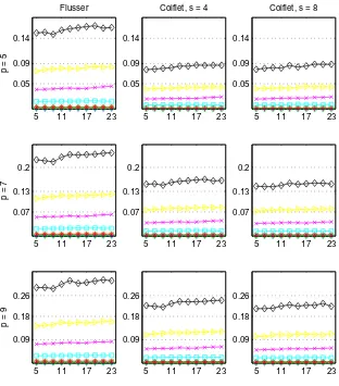
2.2 Median of similarity measures calculated for Flusser’s invariants and the proposed invariants with Coiflet wavelet of order 1 at scales 4 and 8. Every plot shows the effect of different levels of noise. The x-axis represents N, which is the number of neighbourhood for averaging, and they-axis shows the similarity measureR. . . 18

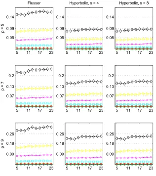
2.3 Median of similarity measures calculated for Flusser’s invariants and the proposed invariants with Hyperbolic wavelet of order 4 at scales 4 and 8. Every plot shows the effect of different levels of noise. The x-axis represents N, which is the number of neighbourhood for averaging, and they-axis shows the similarity measureR. . . 19

2.4 The two EEG signals that are used in experiment 1. . . 23

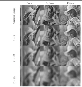
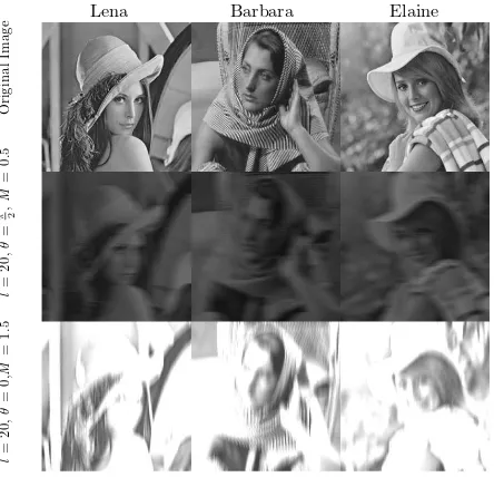
2.5 Images of Lena, Barbara, and Elaine in their original shape and blurred with disk filters of different radii. . . 35

2.6 Images of Lena, Barbara, and Elaine in their original shape and blurred with motion filters of different directions and energies. . . 36

2.7 Ten images from COIL100 database that are used in the second experiment. . . 36

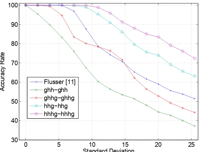
2.8 Accuracy rate in the presence of Gaussian noise. . . 37

2.9 Accuracy rate in the presence of salt and pepper noise. . . 38

2.10 The magnitude responses of the filters used in the second experiment. . . 38

(14)

LIST OF FIGURES

2.12 The registration results with spatial domain blur invariants (SDBI) and wavelet

do-main blur invariants (WDBI). Using SDBIs, one of the images is not registered

cor-rectly, while using WDBIs did not cause any problem. . . 40

3.1 The face recognition architecture that is used in this thesis . . . 45

3.2 Samples from the AT&T database . . . 46

3.3 A face image from the AT&T database blurred with Gaussian filters of different sizes.

σ= 0 is the case for the sharp image. . . 47

3.4 Classification accuracy rate on the AT&T database when artificially blurred with

Gaussian filters. The spatial and wavelet domain blur invariants neither show a good

discriminative power, nor they are invariant to blur effect. Eigenface approach shows

a better classification rate comparing to the blur invariants, however, as it is expected,

is less tolerable to blur. . . 47

3.5 BIDs of a face image obtained with a 8×8 window. They are rescaled for representation. 49

3.6 BID05 of the images in Figure 3.3 obtained with (a) a 8×8 window (b) a 64×64

window. They are rescaled for representation. . . 50

3.7 The distance betweenBIDM×M

05 of a face image and those of the blurred ones where

M = 8 : 4 : 64. . . 51

3.8 The Scheme for Eigenmoment Approach . . . 52

3.9 The Scheme for Local Histogram Approach . . . 53

3.10 Accuracy rate of the EM scheme for the AT&T database. It shows the accuracy rate

for different standard deviations and window sizes. . . 54

3.11 Accuracy rate comparison on the AT&T database versus blur intensity . . . 55

3.12 Accuracy rate of the local histogram scheme for the AT&T database. It shows the

accuracy rate for different standard deviations and window sizes. . . 56

3.13 Accuracy rate comparison on the AT&T database versus blur intensity. LH stands

for local histogram. . . 56

3.14 Samples from the FRGC 1.0.4 experiment . . . 57

(15)

List of Tables

2.1 Eleventh order invariants of an artificial signal that was used in experiment I. The

invariants are shown for different levels of noise variances and two numbers of

neigh-bourhoods in averaging. The scale,s, is 2. . . 20

2.2 Invariants of the EEG signals degraded with different blur systems. The wavelet filter

is Daubechies of order two at level ghh. O.M. stands for the order of magnitude of

the blur invariants. N is the number of neighbourhoods in averaging. N = 0 refers

to the original signal. . . 24

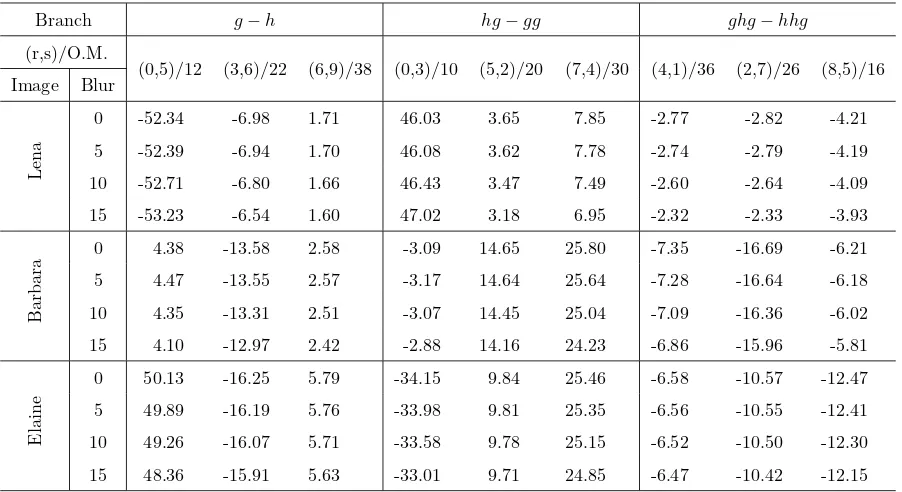
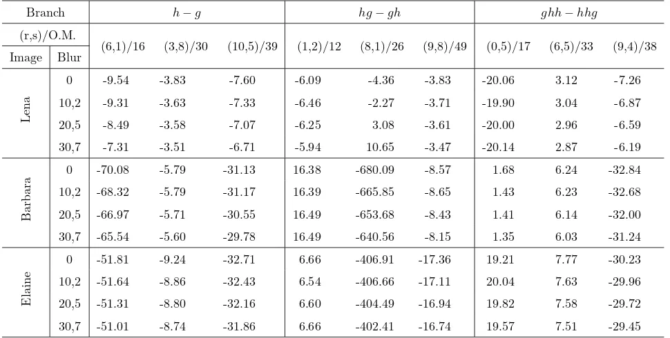
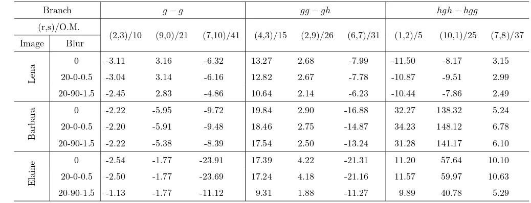
2.3 blur invariants of degraded images with disk filters. Coiflet of order 1 is employed for

this experiment. . . 32

2.4 blur invariants of degraded images with Gaussian filters. Coiflet of order 2 is employed

for this experiment. . . 33

2.5 blur invariants of degraded images with motion, non-energy-preserving filters. Daubechies

of order 3 is employed for this experiment. . . 34

(16)

List of Abbreviations

1D One Dimensional 2D Two Dimensional

BID Blur Invariant Descriptor CWT Continuous Wavelet Transform DSP Digital Signal Processing DWT Discrete Wavelet Transform EEG Electroencephalography EM Eigen Moment

GOM Generalized Ordinary Moment JPEG Joint Photographic Experts Group LH Local Histogram

LPQ Local Phase Quantisation NN Nearest Neighbour

PCA Principal Component Analysis PSF Point Spread Function

(17)

Chapter 1 Introduction and Preliminary Concepts

and Definitions

1.1 Introduction

The face is known to be a very important communication channel in our daily lives, through which

we express our feelings and understand others’, recognize people, and so on. Such abilities are so

integrated in our brain that we do not even realize what a complicated task is being done.

The face is indeed the most favourable biometric feature that everyone carries around with no will of

losing it, making it an easy and non-invasive medium for identification, recognition, human-computer

interaction, to call a few. Such unique properties have caused a growing demand in automatic face

recognition systems by governments, banks, law enforcement, airports, etc., and the accessibility of

powerful computers and fast networks made the realization of such systems only a pattern recognition

problem.

In its simplest setup, the face recognition problem tries to identify an individual from a set of images

of different people. The images are mostly taken in controlled environments, in order to avoid pose

and illumination variations. The currently available face recognition systems report relatively higher

recognition rate in comparison with human on such databases.

However, our natural embedded face recognition system proves to be more robust as soon as the

(18)

1. INTRODUCTION AND PRELIMINARY CONCEPTS AND DEFINITIONS

face expression, occlusion, make-up, and natural processes such as ageing and weight changes are a

few challenges that are encountered by practical face recognition systems. Some of these challenges

have received attention of researchers in the field. For example, pose and illumination variations

are two topics that have been studied comprehensively, and there is even a designated database for

them [22].

On the other hand, other topics have not been addressed. Ageing, for example, is a challenge

that face recognition systems need to deal with as they must accommodate such changes by their

subjects. However, the lack of a suitable database to this date has hindered a real-world study on

this issue, forcing the researchers to synthetically model it [40]. Another recently raised concern is

the vulnerability of automatic face recognition systems to cosmetic surgery [29]. The logic behind

this issue is as the same as the one for ageing, plus the fact that the probability of being caught in

such a situation is low. However, if a bank wants to use such systems to identify their costumers,

they are required to respect their decision, and that leads to a challenge that should be accepted by

the researchers.

Contrastingly with the issues that might be considered as the worries of tomorrow, blur, which is one

of the inevitable challenges in unconstrained face recognition problems[9], has been overlooked until

recently. Movement of the subject, an unfocused camera, or a long distance between the subject

and the camera introduce blur to the acquired image, which can drastically affect the performance

of a face recognition system. Having robust to blur or blur invariant techniques that can tackle such

problems sounds necessary. Most of the techniques that have been proposed so far are based on

deblurring the query image prior to recognition, which requires a preprocessing step and translates

into extra computation. With an increasing volume of videos from surveillance cameras and the need

of going through a lot of them to find a suspect in some instances, a deblurring step before recognition

is definitely not a reasonable idea. Thus, using features that are robust or even better, invariant

-to blur is an alternative approach that can eliminate the need for such tedious preprocesses.

The first category of blur invariants [18] was introduced for the first time with a similar intention:

to avoid deblurring which is an ill-posed problem. The proposed blur invariants were developed

based on geometric moments and in the spatial domain. It was not almost until ten years later

when other researchers showed interest in developing such features as well, but unfortunately most

of their efforts were shown to be redundant [30]. Along with the moment based blur invariants,

another set of such invariants were developed in the Fourier domain [18]. Unlike the first set, the

proposed modifications and extensions on this set of invariants are promising.

(19)

in challenging pattern recognition problems. Most of the applications that have been reported

for these invariants are image registration and remote sensing [20]. This became a motivation

to use these invariants for face recognition to explore their performance in such problems. Also,

the available blur invariants are developed either in the spatial domain or Fourier domain, which

raises this question: is it possible to develop blur invariants in the wavelet domain in order to take

advantage of the extra properties that this domain has? In the next chapter, moment based blur

invariants in the wavelet domain are proposed for the first time as an answer to this question. In

chapter 3, the moment based blur invariants are employed for face recognition. Also an alternative

way of dealing with moments is proposed in that chapter in order to increase their discriminablity,

which yields promising results.

The preliminary definitions and concepts that are required in this dissertation are given in the next

two sections. Section 1.2 is dedicated to wavelet transform. In this section, the general concepts

of wavelet transform are reviewed, and three different types of wavelet transforms for 1D and 2D

signals are presented. Section 1.3 provided a review of geometric moments for 1D and 2D signals.

1.2 Wavelet Transform

Wavelet transform [12] has been used widely in many fields such as JPEG2000 [70]. A growing

number of publications deal with hardware implementation of this transform [60, 33, 49, 66] which

demonstrate its utility in the area of DSP and Pattern Recognition. A multi-resolution analysis

of signals with localization in both time and frequency is the advantage of wavelet transform over

Fourier and cosine transforms [12, 48]. Also, having different alternatives for the basis function in

wavelet transform makes it more adaptable for different problems than Fourier transform since in

the latter only one kind of basis function can be used.

In the rest of this section, continuous and discrete wavelet transforms are reviewed. Also, a specific

type of discrete wavelet transform is introduced, which is shift invariant.

1.2.1 Continuous Wavelet Transform

The continuous wavelet transform (CWT) of a 1D continuous signalf(x) at shiftuand scaleswith

wavelet functionψ(x) is [46]

ˆ

fψ(s, u) = Z +∞

−∞

1

√

sf(x)ψ

∗

x−u s

dx. (1.1)

whereψ∗

(20)

1.2.2 Discrete Wavelet Transform

The wavelet coefficients of 1D discrete signalxare calculated with a cascade of discrete convolutions

and sub-sampling.

aj+1[n] = ¯h ⋆ aj[n]

↓2, (1.2)

dj+1[n] = (¯g ⋆ aj[n])↓2, (1.3)

wherea0=x,j= 0,· · ·, J−1,handg are scaling and wavelet filters, respectively, ¯h[n] =h∗[−n],

and ¯g[n] =g∗

[−n]. aj+1 is the approximation coefficient and dj+1 is the detail coefficient at level

j+ 1.

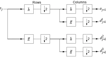
Ifxis a 2D discrete signals, the wavelet coefficients are calculated as follows:

aj+1[n1, n2] = ¯h¯h ⋆ aj[n1, n2]↓2, (1.4)

d1j+1[n1, n2] = ¯hg ⋆ a¯ j[n1, n2]↓2, (1.5)

d2_j+1[n1, n2] = ¯g¯h ⋆ aj[n1, n2]

↓2, (1.6)

d3j+1[n1, n2] = (¯gg ⋆ a¯ j[n1, n2])↓2. (1.7)

where a0 = x, j = 0,· · · , J−1, aj+1 is the approximation coefficient, anddij+1 is the ith detail

coefficient at levelj+ 1. The block diagram of the discrete wavelet decomposition is illustrated in

Figure 1.1.

1.2.3 Shift Invariant Discrete Wavelet Transform

DWT suffers from a major drawback: it is not shift invariant (also called translation invariant in

the literature), and this is due to the dyadic sub-sampling [47, 31]. In order to make the moments

2

2 Columns Rows

j

a aj₊1

1 1 +

j d

2 1

+

j

d

3 1

+

j

d h

g

h

h g

g

(21)

invariant to shift, it is necessary to have a shift invariant wavelet transform. There have been several

different techniques developed to produce shift invariant wavelet transforms. Continuous Wavelet

Transform (CWT) does not suffer from the same drawback as its counterpart in the discrete domain

[46]. Therefore, it is typically utilized when the wavelet transform is only required at a few specific

scales. Mallat proposed a scheme [45] that is an approximation of CWT, which was later proved

to be shift invariant[67]. A trous` algorithm [46] is the simplest and yet an effective technique

that is proposed to make DWT invariant to shift. In this technique, the sub-sampling operator

is removed, and the filters are instead up-sampled at each level by inserting zeros between every

two coefficients [46]. Over Complete DWT (OCDWT) [6] is another proposed technique which

guarantees an approximately shift invariant implementation of wavelet transform if the level below

is fully sampled. Shift invariance has been also achieved by calculating the wavelet transform of all

shifts [34].

In this dissertation, the `a trousalgorithm is used. In this algorithm, scaling and wavelet filters at

scalej+ 1 are defined as

hj+1[k] =hj[k]↑2 =  



hj[k₂], k even

0, k odd

(1.8)

gj+1[k] =gj[k]↑2 =  



gj[k

2], k even

0, k odd

(1.9)

where h0[k] =h[k] and g0[k] = g[k]. The wavelet coefficients of 1D discrete signalxare calculated

with a cascade of discrete convolutions.

aj+1[n] = ¯hj⋆ aj[n], (1.10)

dj+1[n] = ¯gj⋆ aj[n], (1.11)

where a0 =x, j = 0,· · ·, J−1. In this dissertation, the wavelet coefficients (either approximation

or detail) of signalxat levelf0f1· · ·fL−1 are called

ψL

W x, which is related toxas

ψL

W x[n] = ¯ψL⋆ x[n], (1.12)

where

(22)

Columns Rows

j h

j g j

g

j g j

a aj₊1

1 1

+

j

d

2 1

+

j d

3 1

+

j d

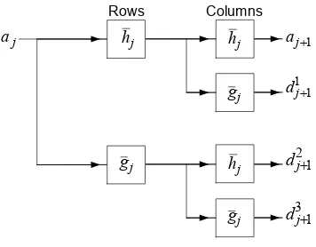
Figure 1.2: Decomposition in Redundant Wavelet Transform

andf is eitherhorg.

Similarly, ifxis a 2D discrete signal, its wavelet coefficients are calculated as follows:

aj+1[n1, n2] = ¯hjh¯j⋆ aj[n1, n2], (1.14)

dj1+1[n1, n2] = ¯hjg¯j⋆ aj[n1, n2], (1.15)

d2_j+1[n1, n2] = ¯gj¯hj⋆ aj[n1, n2], (1.16)

d3j+1[n1, n2] = ¯gj¯gj⋆ aj[n1, n2]. (1.17)

wherea0=x, andj = 0,· · ·, J−1. The block diagram of this transform is presented in Figure 1.2.

The wavelet coefficients (either approximation or detail) of signalxat levelf1

0f11· · ·fL1−1−f02f12· · ·fL2−1

are calledW xψL, which is related toxas

ψL

W x[n1, n2] = ¯ψL⋆ x[n1, n2], (1.18)

where

ψL[n1, n2] =ψL1[n1]ψL2[n2], (1.19)

ψ1

L[n1] =f01⋆· · ·⋆ fL1−1[n1], (1.20)

ψ2_L[n2] =f02⋆· · ·⋆ fL2−1[n2], (1.21)

(23)

1.2.4 Vanishing Moment

The wavelet functionψ∈L2₍_Z_{) has}_M

ψ vanishing moments (also called zero moments) if

Z +∞

−∞

tp_ψ₍_t₎_dt_{= 0}_, _for_p_≤_M

ψ. (1.22)

The number of vanishing moments ofψis equal to the number of zeros of its Fourier transform, ˆψ(w),

at w= 0 [46]. Mψ depends on the number of zeros ofg’s Fourier transform, ˆg(w), at w= 0,Mg,

and its repetition in obtainingψ,N. Since the scaling filter designed such that ˆh(0) =√2, we can

easily show that Mψ =N Mg. Therefore, ifψL ∈L2 Z2, and it consists ofNi wavelet filters on theith _{dimension (}_i_{= 1}_,_{2), then it has}_M

ψi

L =NiMg on that dimension.

1.3 Moments

In this section, some of the basic terms for moments are defined and explained.

1.3.1 Moments for Continuous Signals

The pth _{order ordinary geometric moment of 1D continuous signal} _f₍_x_{) in the spatial domain is}

defined by [59]

mfp= Z +∞

−∞

xpf(x)dx. (1.23)

The centroid of signalf(x) is [59]

cf ₌m f

1

mf0

. (1.24)

Thepth _{order central moment of 1D continuous signal}_f₍_x_{) in the spatial domain is defined by [59]}

µf p =

Z +∞

−∞

x−cfp_f₍_x₎_dx. _(1.25)

1.3.2 Moments for Discrete Signals

Thepth _{order ordinary geometric moment of 1D discrete signal}_x_{in the spatial domain is defined}

by

mx p =

X

n

np_x_[_n_]_. _(1.26)

The centroid of signalxis

cx₌ mx1

mx

0

(24)

Thepth _{order central moment of 1D discrete signal}_x_{in the spatial domain is defined by}

µx p=

X

n

(n−cx₎p_x_[_n_]_. _(1.28)

If the discrete signalxis 2D, its ordinary geometric moment of order (p+q) in the spatial domain

is defined by

mxp,q = X

n1 X

n2

np1n

q

2x[n1, n2]. (1.29)

The centroid of signalxis

cx1=

mx

1,0

mx

0,0

, cx2 =

mx

0,1

mx

0,0

. (1.30)

The central moment of order (p+q) of 2D discrete signalxin the spatial domain is defined by

µx p,q=

X

n1 X

n2

(n1−c1)p(n2−c2)qx[n1, n2]. (1.31)

It is worth mentioning that there are some other definitions available for moments which happen

to be orthogonal as well. However, only geometric moments are exploited in this dissertation for

proposing new algorithms. This does not deny the possibility of developing them based on orthogonal

(25)

Chapter 2 Blur Invariants: A Novel Representation

in the Wavelet Domain

2.1 Introduction

Signal acquisition is the first step in all signal processing tasks, and is always accompanied with

different sources of degradation. The effect of some of the degradations is considerably high, which

could vastly affect expected outcomes. People in surveillance photos and body parts in medical

im-ages are real-world subjects that are not ideally controllable when acquiring imim-ages. Environmental

situations might also have a negative effect on the quality of signals, e.g. weather condition and long

distances between camera and subject can deteriorate images. Deteriorations in images are basically

of two types: geometric distortions, and radiometric degradations. The first type includes the

dis-tortions such as translation, scaling, and rotation. There are many different approaches in literature

which are proposed for dealing with these problems. Hu, for the first time, proposed descriptors

that are invariant to some of the basic linear geometric distortions [26]. Recently a novel approach

has been put forward by Flusser et al. [15], where implicit moment invariants are introduced for

dealing with nonlinear deformations. For surveys on similar invariants refer to [64, 74, 20].

Unlike geometric distortions, there are fewer research works carried out on radiometric degradations.

They are generally introduced to images due to the movement of subject, unfocused camera, and

(26)

2. BLUR INVARIANTS: A NOVEL REPRESENTATION IN THE WAVELET DOMAIN

signal is

g(x) =Hf(x) +n(x) (2.1)

In this model, g is the observed signal,f and n are the actual signal and noise, respectively, and

H is the degradation operator. It is assumed thatH is linear and space-invariant, and the general

model can be simplified to

g(x) =f(x)⋆ h(x) +n(x), (2.2)

where ‘⋆’ denotes the convolution, andhis the Point Spread Function (PSF) of the system.

The proposed approaches for dealing with blur can be categorized into two types: 1) blind

restora-tion, and 2) direct analysis. In blind restoration techniques, the purpose is to identify the blur system

model and extract the actual signal [65, 32]. The main application of these methods is in signal

restoration. There are also similar techniques in which the effort is to only restore the features of

degraded signals [23], with their main application in pattern recognition. Although these techniques

have been vastly used, they suffer from major drawbacks: deblurring is an ill-posed problem, and

because of the identification part, they are computationally expensive, while it is not required to

identify the blur system in many applications.

The second type of techniques focus on developing descriptors that are inherently invariant to blur.

The main advantage of these methods is that they do not go through the process of identifying

the blur system. Flusser et al. [18] established this type for the first time. Their invariant

de-scriptors were developed in the spatial domain and based on geometric moments. Their assumption

was that the blur operator is symmetric. Later, they represented a closed format of the invariants

[19], and added extra properties to the descriptors in order to make them invariant to geometric

distortions while changing their assumption for the blur systems to centrally symmetric[17, 69].

They also developed these invariants for 1D signals [16]. Utilizing complex moments, Flusser and

Zitov`a [21] proposed descriptors that are both invariant to centrally symmetric blur and rotation.

Liu and Zhang [39] also developed similar blur invariants using complex moments. Metari and

De-schˆenes [50] exploited the Mellin transform properties in order to define a different representation of

geometric-moment-based blur invariant descriptors. They also showed that their proposed

descrip-tors are invariant to a few geometric distortions as well. Instead of using geometric moments, Zhang

et al. [76] employed Legendre moments in order to define their invariants in the spatial domain. On

the other hand, Ji and Zhu [28] proved that the Zernike moments ,Zpq, are inherently invariant to

Gaussian blur whenp=q.

Along with the blur invariant descriptors defined in the spatial domain, there are some other

(27)

invariants for 1D signals based on the tangent of the phase of signals, and proved that they are

invariant to blur. They developed this representation for 2D signals and showed their relationship

with their invariants in the spatial domain [17]. These invariants were later developed fornD signals

and made to be invariant to some of the geometric distortions [14]. Ojansivu and Heikkil¨a [57],

how-ever, showed that Flusser’s invariants are sensitive to noise when implemented in the Fourier domain

because of their use of tangent operator. They proposed a different representation of invariants in

the Fourier domain. Subsequently, they made them invariant to the affine transform as well [56].

Blur moment invariants showed their practicality in a vast area of research: image registration

[17, 55], remote sensing [5, 4], forgery detection [41], recognition [19, 39, 10], stereo matching [61],

and control point extraction [3].

In this chapter, wavelet domain descriptors are proposed which are invariant to centrally symmetric

blur systems. The immediate advantages of these invariants come from the domain that they are

developed in: the different alternatives that exist for wavelet functions and the benefit of analysing

signals at different scales in the wavelet domain. The wavelet domain blur invariants are first

de-veloped for 1D continuous signals. With a slight modification they are also presented for 1D and

2D discrete signals. This chapter is organized as follows. In section 2.2, the representation of blur

in the wavelet domain for 1D continuous signals is shown first. Then, the relationship between the

moments of the blurred signal in the wavelet domain and those of the original signal in the same

domain are extracted. Using this relation, the blur invariants for 1D continuous signals are proposed

and proved. The performance of these invariants is evaluated in section 2.3 against noise and blur

changes and compared with the performance of the spatial domain blur invariants. Section 2.4 is

devoted to extracting blur invariants for 1D discrete signals. In section 2.5, the performance of the

developed invariants is evaluated in an experiment with two electroencephalography (EEG) signals.

The wavelet domain blur invariants for 2D discrete signals are proposed in section 2.6, and analysed

comprehensively in section 2.7 in three different experiments. There might be some special cases

where the spatial domain and wavelet domain blur invariants cannot discriminate different signals.

This discussion comes in section 2.8. The chapter is concluded in section 2.9.

2.2 Blur Invariants for 1D Continuous Signals

For 1D continuous signals, the wavelet transform is calculated with CWT (eq. 1.1), and the moments

(28)

2.2.1 Blur in the Wavelet Domain for 1D Continuous Signals

First, it will be shown that how (2.2) would be presented in the wavelet domain. Also for the sake

of simplicity, noise is not shown in the equations. However, its effect on the invariants will be shown

in section 2.3. The wavelet transform of blurred continuous signalg(x) at shiftuand scale swith

wavelet functionψ(x) is

ˆ

gψ(s, u) = Z +∞

−∞

1

√

sg(x)ψ

∗

x−u s

dx. (2.3)

Replacingg(x) by its equivalent in (2.2) gives

ˆ

gψ₍_{s, u}_{) =} Z +∞

−∞ Z +∞

−∞

1

√

sh(y)f(x−y)ψ

∗

x−u s

dydx. (2.4)

Substituting zforx−y, the above equation changes to

ˆ

gψ₍_{s, u}_{) =}

Z +∞

−∞

h(y) Z +∞

−∞

1

√

sf(z)ψ

∗ _z

−(u−y)

s dzdy = Z +∞ −∞

h(y) ˆfψ₍_{s, u}₋_y₎_dy _(2.5)

which shows that the wavelet transform ofg(x) is the convolution of h(x) by the wavelet transform

off(x):

ˆ

gψ₍_{s, u}_{) = ˆ}_fψ₍_{s, u}₎_{⋆ h}₍_u₎_. _(2.6)

2.2.2 Moments in the Wavelet Domains for 1D Continuous Signals

Before expressing the relation between the moments of ˆgψ₍_{u, s}_{) and those of ˆ}_fψ₍_{u, s}_{) and}_h₍_u_{), it is}

shown how the moments off(x) in the wavelet domain are related to those in the spatial domain.

Rewriting moments of continuous signals (eq. 1.3) for ˆfψ₍_{u, s}_{), the wavelet transform of} _f₍_x_{) with}

wavelet functionψ(·) at shiftuand scales, we have the following:

mfˆψ p (s) =

Z +∞

−∞

up_f_ˆψ₍_{s, u}₎_du

= √1

s

Z +∞

−∞ Z +∞

−∞

up_f₍_x₎_ψ∗

x−u s

dxdu

= √s

Z +∞

−∞ Z +∞

−∞

(x−sy)pf(x)ψ∗

(y)dxdy. (2.7)

In (2.7), y is substituted for x−u s

. Considering the fact that (a+b)p = Pp_k₌₀ p_kak_bp−_k

, the

relation between the ordinary moments of signalf(x) in the wavelet domain and the spatial domain

can be extracted:

mfpˆψ(s) = p X k=0 p k

sk+12(−1)kmf

p−km ψ

(29)

It can be concluded from (2.8) that the moments of the wavelet transform of a signal with a wavelet

function which has Mψ vanishing moments are zero up to order Mψ−1. Therefore, it would be

impossible to calculate the centroid (eq. 1.24) for such signals since the denominator can become

zeros. This also makes it impossible to take advantage of central moments. In order to be able to

take advantage of central moments for such signals, a generalized definition of centroid is proposed,

which appeared in [42] for the first time.

Definition 1. If the moments of signalf(x)are zero up to orderM −1, its centroid is defined as

ςf ₌ m

f M+1

(M+ 1)mf_M. (2.9)

It is trivial to show thatcf _{is a special case of}_ςf_{, where}_M _{= 0.}

The relation between thepth _{order central moment of ˆ}_gψ₍_{s, u}_{) and the central moments of ˆ}_fψ₍_{s, u}₎

and h(x) can be extracted by rewriting (1.25) for ˆgψ₍_{s, u}_{) with the generalized centroid definition}

(2.9), using (2.6), and considering the fact thatςgˆψ

=ςfˆψ

+ch_.

µˆgψ p (s) =

Z +∞

−∞

u−ςˆgψp_g_ˆψ₍_{s, u}₎_du

=

Z +∞

−∞ Z +∞

−∞

u−ςgˆψp_f_ˆψ₍_{s, u}₎_h₍_v₋_u₎_dvdu

= p X

k=0

p k

µf_kˆψ(s)µh

p−k. (2.10)

If the employed wavelet function hasMψvanishing moments, by definingq+Mψ=p, ´µq(s) =µp(s),

and q_l_M

ψ =

q+M ψ l+M ψ

, the above equation can be simplified into:

´

µgˆψ q (s) =

q X

l=0

q l

Mψ

´

µf_lˆψ(s)µh

q−_l. (2.11)

It shows that the central moments of ˆgψ₍_{s, u}_{) of a certain order are related to the central moments}

of ˆfψ₍_{s, u}_{) and}_h₍_x_{) of the same and lower orders.}

2.2.3 Wavelet Domain Blur Invariants for 1D Continuous Signals

In order to extract blur invariant features, it is necessary to look for combinations of moments such

that those ofh(x) would be eliminated. It is assumed thath(x), the PSF, is symmetric and

energy-preserving. When h(x) is symmetric, i.e. h(x) = h(−x), its odd order moments are zero. And

because of the energy-preserving property, the integralR−∞+∞h(x)dx, which isµ

h

(30)

Theorem 1: Ifqis odd, thenCq(s), which is defined as follows, is invariant to blur in the wavelet

domain with wavelet functionψ(·).

Cq(s) = ´µq(s)− 1

´

µ0(s) q−1

2 X

l=1

q q−2l

Mψ 2l 0 Mψ

Cq−2l(s) ´µ2l(s) (2.12)

Proof _When_q_{= 1,}_Cgˆψ

1 (s) =C ˆ

fψ 1 (s) = 0.

Forq= 3, it can be trivially shown thatC₃gˆψ(s) =C₃fˆψ(s).

C3ˆgψ(s) = µ´ ˆ

gψ 3 (s)

= 3 X l=0 ₃ l Mψ ´

µf_lˆψ(s)µh3−l

= µ´f₃ˆψ(s) =C₃fˆψ(s). (2.13)

If (2.12) is valid for 1,3, ..., q−2, it can be proved that it is valid forqas well:

Cˆgψ

q (s) = µ´

ˆ

gψ

q (s)− 1 ´

µˆg0ψ(s) q−1

2 X

l=1

q q−2l

Mψ 2l 0 Mψ

C_qgˆ−ψ2l(s) ´µ

ˆ

gψ

2l(s)

= q X

k=0

q+Mψ

k

´

µf_qˆ−ψk(s)µ h k

− 1

´

µf0ˆψ(s) q−1

2 X

l=1

q q−2l

Mψ 2l 0 Mψ

C_qfˆ₋₂ψ _l(s)

2l X

k=0

₂_l₊_M ψ

k

´

µf₂ˆ_lψ−k(s)µ h k

= Cfˆψ q (s) +

q X

k=1

q+Mψ

k

´

− 1

´

µf₀ˆψ(s)

q−1 2 X

l=1

q q−2l

Mψ 2l 0 Mψ

C_qfˆ−ψ2l(s)

2l X

k=1

2l+Mψ

k

´

µf₂ˆ_lψ−k(s)µhk

= Cfˆψ

q (s) + q X

k=1

_q₊_M ψ

k

´

− 1

´

µf0ˆψ(s) q−1

2 X l=1 2l X k=1

2l+Mψ

k

q

q−2l Mψ 2l 0 Mψ

C_qfˆ−ψ2l(s) ´µ

ˆ

fψ

2l−_k(s)µ

h k

= Cqfˆψ(s) + q X

k=1

q+Mψ

k

´

− 1

´

µf0ˆψ(s)

q−1 X

k=1 q−1

2 X

l=[k+1

2 ]

_q₊_M ψ

k

q−k q−2l

Mψ 2l−k

0

Mψ

C_qfˆ−2ψ l(s) ´µ

ˆ

fψ 2l−k(s)µ

h k

= Cqfˆψ(s) +

q+Mψ

q

´

µf0ˆψ(s)µhq q−1 X

k=1

q+Mψ

k

(31)

× 

µ´fˆ

ψ

q−k(s)− 1

´

µf₀ˆψ(s)

q−1 2 X

l=[k+1

2 ]

q−k q−2l

Mψ 2l−k

0

Mψ

C_qfˆ−ψ2l(s) ´µ

ˆ

fψ

2l−k(s) 



= Cfˆψ q (s) +

q+Mψ

q

´

µf₀ˆψ(s)µh q +

q−1 X

k=1

q+Mψ

k

µh

kJq,k(s). (2.14)

Whenk is odd,µh

k is zero. Hence, the second term in (2.14) becomes zero. The only term in (2.14) that is dependent on the moments ofhis Jq,k(s). In order to prove that the proposed invariant is

independent of PSF, it is necessary to show that whenkis even,Jq,k(s) = 0 .

Jq,k(s) = µ´

ˆ

fψ

q−k(s)− 1

´

µf0ˆψ(s) q−1

2 X

l=k 2

q−k q−2l

Mψ 2l−k

0

Mψ

C_qfˆ₋₂ψ _l(s) ´µf₂ˆ_lψ−k(s)

= µ´f_qˆ−ψk(s)− 1

´

µf₀ˆψ(s)

q−k−1 2 X

l=0

q−k q−k−2l

Mψ 2l 0 Mψ

C_qfˆ−ψk−2l(s) ´µ

ˆ

fψ 2l(s)

= µ´f_qˆ−ψk(s)− 1

´

µf0ˆψ(s) q−k−1

2 X

l=1

q−k q−k−2l

Mψ 2l 0 Mψ

C_qfˆ−ψk−2l(s) ´µ

ˆ

fψ 2l(s)

− 1

´

µf0ˆψ(s)

q−k q−k Mψ 0 0 Mψ

C_qfˆ−ψk(s) ´µ

ˆ

fψ 0(s)

= C_qfˆ−ψk(s)−C

ˆ

fψ

q−k(s)

= 0. (2.15)

SinceJq,k(s) is zero whenkis odd, the only remaining term in (2.14) isCfˆψ

q (s). Therefore,Cqˆg(s) =

Cfˆ

q(s). 2

Corollary 1: Flusser’s invariants [16] are a special case of (2.12).

Proof _{To obtain Flusser’s invariants, it is assumed that} _ψ₍_·_{) is the Dirac delta function. In this}

case,Mψ = 0 which implies thatψ(·) is not a wavelet function anymore. Therefore,p=q+Mψ=q

and µp= ´µq. By settings= 1 at all time, it is trivial to show that ˆfψ(x,1) is equivalent to f(x),

since the signal is convolved by the Dirac delta function. From here, (2.12) is rewritten with the

new assumptions.

Cpf = µp− 1

µ0 p−1

2 X

l=1

p p−2l

0 2l 0 0

C_pf−2lµ2l

= µp− 1

µ0 p−1

2 X

l=1

_p

p−2l

C_pf−2lµ2l. (2.16)

(32)

2.3 Experiment 1: Blur and Noise Analysis

In this section, the performance of the proposed invariants is demonstrated by applying it to 1D

signals, and comparing to Flusser’s invariants [16]. Two different types of wavelet functions were

employed to demonstrate the performance of the invariants under the change of this parameter. The

first wavelet function is Coiflet of order 1 (Mψ= 2) [11]. There is no closed-form representation for

this orthogonal wavelet. The second wavelet function belongs to the crude wavelet class. The wavelet

function that is employed here is a hyperbolic kernel , which, unlike Coiflet, has an explicit expression

(2.17). This wavelet function is comprehensively studied in [35, 36, 37], and different properties are

extracted. For the experiments of this section,nandβ were set to 4 and 1 respectively. This wavelet

function has two vanishing moments as well.

ψn,β(x) =−nβ2sechn(βx) n−(n+ 1) sech2(βx) (2.17)

For this experiment, 1000 1D signals with the length of 200 and in the range of [-1 1] were artificially

generated. Figure 2.1 shows one of the signals. The signals were blurred by calculating N-point

neighbourhood averaging with a neighbourhood of 5, 7, 9, 11, 13, 15, 17, 19, 21, and 23. In order

to study the effect of noise on the performance of the invariants, the signals were also contaminated

with additive noise. The added noise was Gaussian with zero mean and the standard deviation of

0 (no noise), 0.001, 0.002, 0.008, 0.02, 0.04, and 0.08. The wavelet transform of the signals were

obtained with the wavelet functions described above at 3 scales,s= 2, 4, and 8. The invariants for

all of the original and blurred signals were calculated up to order 11 (q = 9, p=q+Mψ = 11).

However, the invariants of order 3 (q= 1, p=q+Mψ = 3) are not reported since they are zero.

Then, based on the following equation, the similarity between the original signals and their blurred

versions was measured

R=

CX p −CpO

CO p

(2.18)

where CO

p and CpX are the pth order invariants of the actual and blurred signals respectively. The closerCX

p is toCpO, the smallerR becomes.

Figures 2.2 and 2.3 show the medians of the similarity measures for invariants obtained with Coiflet

and hyperbolic wavelet functions respectively. Both figures show invariants of three orders: 5, 7,

and 9, and consists of 9 plots: 3 representing the results acquired with Flusser’s invariants, and

the other 6 results with the proposed invariants at two scales: 4 and 8. Every plot has several

graphs representing different levels of noise. Thex−axis represents the number of neighbourhoods

(33)

0 50 100 150 200

−1 −0.5 0 0.5 1

Figure 2.1: One of the artificial signals that was used in experiment I.

invariants are repeated in both figures for the sake of comparison. Also, Table 2.1 shows the eleventh

order invariants of one the signals for different levels of noises.

The first noticeable property of the invariants is that by increasing the order of the invariants,R

increases as well. The reason of this rise is because the invariants also increase exponentially with

respect to their order.

By changing the noise level, the similarity changes from 0% to 30% in Flusser’s invariants and 25%

in the wavelet based invariants, which is 5% less than the one in the spatial domain (Figures 2.2

and 2.3). The wavelet based invariants show a generally better robustness than Flusser’s invariants

in this experiment. However, it is impossible to make a general statement about the robustness of

invariants in the wavelet domain than those in the spatial domain. The reason is that there are

various wavelet functions available with different properties, which requires a comprehensive study

of its own.

A slight increase in similarity is observable by the increase of N in Flusser’s invariants. It is also

noticeable in the proposed invariants at scale 4, but it becomes less evident for the invariants at

scale 8, specially for invariants with Coiflet. The similarity measure is also slightly less for these

invariants. Since a higher scale is equivalent to a lower resolution, the effect of blur and noise is less

significant. However, the risk of losing the properties of signals also increases. Therefore, a proper

selection of scales is substantial.

Comparing the results obtained by Flusser’s invariants and those of the wavelet based invariants

(34)

5 11 17 23 0.05

0.09 0.14

Flusser

p = 5

5 11 17 23 0.05

0.09 0.14

Coiflet, s = 4

5 11 17 23 0.05

0.09 0.14

Coiflet, s = 8

5 11 17 23 0.07

0.13 0.2

p = 7

5 11 17 23 0.07

0.13 0.2

5 11 17 23 0.07

0.13 0.2

5 11 17 23 0.09

0.18 0.26

p = 9

5 11 17 23 0.09

0.18 0.26

5 11 17 23 0.09

0.18 0.26

Figure 2.2: Median of similarity measures calculated for Flusser’s invariants and the proposed

in-variants with Coiflet wavelet of order 1 at scales 4 and 8. Every plot shows the effect of different

levels of noise. The x-axis representsN, which is the number of neighbourhood for averaging, and

(35)

5 11 17 23 0.05

0.09 0.14

Flusser

p = 5

5 11 17 23 0.05

0.09 0.14

Hyperbolic, s = 4

5 11 17 23 0.05

0.09 0.14

Hyperbolic, s = 8

5 11 17 23 0.07

0.13 0.2

p = 7

5 11 17 23 0.07

0.13 0.2

5 11 17 23 0.07

0.13 0.2

5 11 17 23 0.09

0.18 0.26

p = 9

5 11 17 23 0.09

0.18 0.26

5 11 17 23 0.09

0.18 0.26

Figure 2.3: Median of similarity measures calculated for Flusser’s invariants and the proposed

in-variants with Hyperbolic wavelet of order 4 at scales 4 and 8. Every plot shows the effect of different

levels of noise. The x-axis representsN, which is the number of neighbourhood for averaging, and

(36)

Table 2.1: Eleventh order invariants of an artificial signal that was used in experiment I. The

invariants are shown for different levels of noise variances and two numbers of neighbourhoods in

averaging. The scale,s, is 2.

Noise Flusser Coiflet (s= 2) Hyperbolic (s= 2)

N=7 N=11 N=7 N=11 N=7 N=11

0.000 -1.26e+31 -1.26e+31 5.51e+30 5.51e+30 1.59e+32 1.59e+32

0.001 -1.26e+31 -1.26e+31 5.50e+30 5.50e+30 1.59e+32 1.59e+32

0.002 -1.26e+31 -1.27e+31 5.52e+30 5.53e+30 1.59e+32 1.60e+32

0.008 -1.33e+31 -1.32e+31 5.79e+30 5.74e+30 1.69e+32 1.68e+32

0.020 -1.12e+31 -1.13e+31 4.88e+30 4.92e+30 1.37e+32 1.38e+32

0.040 -1.59e+31 -1.57e+31 6.92e+30 6.84e+30 2.12e+32 2.09e+32

0.080 -9.81e+30 -9.81e+30 4.28e+30 4.28e+30 1.16e+32 1.16e+32

did not have any major influence on the performance of the invariants, but provide a different

range of values (Table 2.1). As it is mentioned above, it is possible that with a different choice of

wavelet function contrary results would be obtained. The application that the proposed invariants

are supposed to be used could have a significant influence on the choice of the wavelet function,

since different types of wavelet functions are sensitive to different properties in signals [46]. It might

be even useful to employ multiple wavelet functions in order to extract different moment invariants

for a comprehensive analysis.

2.4 Blur Invariants for 1D Discrete Signals

DWT is the common appraoch for wavelet decomposition of discrete signals. However, this tool is

not shift invariant. In order to preserve the shift invariance property, the`a trousalgorithm (eq. 1.10

and 1.11) is used. Also, the moment definitions for discrete signals (1.26 - 1.28) are employed in

this section. Having chosen the proper wavelet transform, the representation of blur and moments

(37)

2.4.1 Blur in the Wavelet Domain for 1D Discrete Signals

The wavelet transform of a blurred signal with wavelet functionψL is

ψL

W y[n] = ¯ψL⋆ y[n], (2.19)

where y[n] =b ⋆ x[n], is a discrete representation of (2.2), with bas the blur system, andxas the

original signal. Substitutingy with its equivalent gives

ψL

W y[n] = ¯ψL⋆ b ⋆ x[n]

=b ⋆ψ¯L⋆ x[n] =b ⋆ ψL

W x[n]. (2.20)

Eq. (2.20) implies that the wavelet transform of blurred signaly is the convolution of blur system

bwith the wavelet transform of original signalx.

2.4.2 Moments in the Wavelet Domain for 1D Discrete Signals

The ordinary moment of orderpofW xψL is

m ψL W x p = X n

npW xψL[n]

=X n

X

l

np_x_[_l_]_ψ_L[_l₋_n_{] =}X l

X

k

(l−k)px[l]ψL[k]

= p X i=0 X l X k p i

(−1)ilp−i_x_[_l_]_ki_ψ_L[_k_{] =} p X i=0 p i

(−1)imx p−im

ψL

i , (2.21)

wherel−nis substituted withk. IfψLhasMψL vanishing moments,m

ψL

i in (2.21) will be zero for

i < MψL. This forces the moments of

ψL

W xto also be zero forp < MψL. Considering this and similar to

the case for continuous signals, the generalized definition of centroid (eq. 2.9) can be used in (1.28)

to overcome this problem. Therefore, the central moment of orderpofW yψL is

µ ψL W y p = X n

n−ς

ψL

W y !p

ψL

W y[n] =X n

X

l

n−ς

ψL

W y !p

ψL

W x[l]b[n−l]

=X l

X

k

l−ς

ψL

W x !

+ k−cb !p

ψL

W x[l]b[k]

= p X i=0 X l X k p i

l−ς

ψL

W x !i

ψL

W x[l] k−cbp−i

b[k]

= p X i=0 p i µ ψL W x

(38)

where l−n is substituted with k. Also, it is trivial to show that ς

ψL

W y ₌ _ςW xψL ₊_cb_{. Since} _µW xψL i is zero fori < MψL, pshould be equal to or greater thanMψL. Therefore, by definingq+MψL =p,

´

µq =µp, and a_b_M = a_b+₊_MM, (2.22) is modified to

´ µ ψL W y q = q X i=0 q i M_ψL ´ µ ψL W x

i µbq−i. (2.23)

2.4.3 Wavelet Domain Blur Invariants for 1D Discrete Signals

It is clear from (2.23) that the central moments of a blurred signal are related to those of the original

signal and the blur system. To have wavelet domain blur invariants based on these moments, it is

required to find a combination of them such that the moments of the blur system are not present

any longer.

Theorem 2: ForW xψL, which is the wavelet transform of xwith wavelet function ψL, C

ψL

W x

q is

in-variant to symmetric and energy-preserving blur systems.

C ψL W x q =            ´ µ ψL W x q − 1 ´ µ ψL W x 0 q−1

2 X

l=0

q q−2l

M_ψL 2l 0 M_ψL C ψL W x q−2lµ´

ψL

W x

2l , l is odd

0, l is even.

(2.24)

Proof _{Refer to the proof of Theorem 1.} 2

Theorem 2 is applicable when the blur system is energy-preserving. However, such systems are not

always realistic. The next theorem eliminates this restriction.

Theorem 3: For W xψL, which is the wavelet transform of x with wavelet function ψL, D

ψL

W x q is

invariant to symmetric blur systems.

D ψL W x q =          ´ ν ψL W x q −

q−1 2 X

l=0

q q−2l

M_ψL 2l 0 M_ψL D ψL W x q−2lν´

ψL

W x

2l , l is odd

0, l is even,

(2.25)

whereν´x

q = ´µxq/µ´x0.

Proof _{Assume ˜}_b_{is a non-energy-preserving system. Such systems could be represented as}

˜

(39)

0 100 200 300 400 500

−200 0 200

EEG

Si

g

n

a

l

1

0 100 200 300 400 500

−200 0 200

EEG

Si

g

n

a

l

2

Figure 2.4: The two EEG signals that are used in experiment 1.

where c and b are a constant and an energy-preserving system, respectively. It is trivial to show

thatµ˜b

q =cµbq, and from hereccan be found as the zero order moment of the non-energy-preserving system,µ˜b

0. Remember that the zero order moment of an energy-preserving system is equal to 1.

Assuming that y andz are both blurred versions ofxby blur systems ˜b andb, respectively, it can

trivially be shown that ´ν

ψL

W y_{= ´}_νW zψL_.

Without loss of generality,ν can be replaced in (2.24) to achieve blur invariants with no restriction

on the energy of the system, given in (2.25). It should also be mention that sinceν

ψL

W x

0 becomes 1

for all signals, the term before the summation in (2.24) does not appear in (2.25) any more. 2

2.5 Experiment 2: Blur Analysis

In this section, the blur invariants are evaluated in an experiment with blurred EEG signals. Wavelet

function Daubechies of order 2 (DB2), which has 2 vanishing moments [11], is used in this

exper-iment, and is carried out at level ghh, which means that the wavelet transform of the signals is

obtained by applying the highpass filter followed twice by the lowpass filter.

Figure 2.4 shows the two EEG signals that are used for this experiment. They are chosen from the

database generated by Andrzejak et al. [2]. The signals are blurred by averaging onN

neighbour-hoods, whereN is 11 and 21, and energies of 0.7 and 0.4, respectively.

Table 2.2 represents the invariants of order 5 to 11 of the original signals and their blurred ones.

It is clear that blur intensity and system energy changes do not affect the invariants significantly.

(40)

Table 2.2: Invariants of the EEG signals degraded with different blur systems. The wavelet filter is

Daubechies of order two at levelghh. O.M. stands for the order of magnitude of the blur invariants.

N is the number of neighbourhoods in averaging. N = 0 refers to the original signal.

q/O.M.

5/7 7/13 9/19 11/25

N/m˜b

0

S

ig

.

1 0 56.49 130.22 617.55 4317.66

11/0.7 56.48 130.18 617.25 4314.94 21/0.4 56.53 130.44 618.98 4330.91

S

ig

.

2 0 -0.41 0.21 -0.16 0.19

11/0.7 -0.41 0.20 -0.16 0.19 21/0.4 -0.40 0.20 -0.16 0.18

2.6 Blur Invariants for 2D Discrete Signals

Similar to the case for 1D discrete signals in order to preserve the shift invariance property, it is

required to use the `a trous algorithm (eq. 1.14 - 1.17). Also, the moment definitions for discrete

signals (eq. 1.29 - 1.31) are employed in this section.

2.6.1 Blur in the Wavelet Domain for 2D Discrete Signals

The representation of (2.2) for 2D discrete signals is

y[n1, n2] =b ⋆ x[n1, n2], (2.27)

werey andxare the blurred and original signals, respectively, and bmodels the blur system. The

wavelet transform of a blurred signal with wavelet functionψLis

ψL

W y[n1, n2] = ¯ψL⋆ y[n1, n2]. (2.28)

Substituting ywith its equivalent in (2.27) gives

ψL

W y[n1, n2] = ¯ψL⋆ b ⋆ x[n1, n2]

=b ⋆ψ¯L⋆ x[n1, n2]

=b ⋆W xψL[n1, n2]. (2.29)

Eq. (2.29) implies that the wavelet transform of blurred signaly is the convolution of blur system

(41)

2.6.2 Moments in the Wavelet Domain for 2D Discrete Signals

The ordinary moment of order (p+q) ofW xψL is

m ψL W x p,q = X n1 X n2

np₁nq₂W xψL [n1, n2]

=X n1 X n2 X n3 X n4

np₁nq₂x[n3, n4]ψL[n3−n1, n4−n2]

(n3−n5)p(n4−n6)qx[n3, n4]ψL[n5, n6]

= p X i=0 q X j=0 X n3 X n4 X n5 X n6 p i q j

(−1)i+jnp−_i 3 nq

−_j

4 x[n3, n4]n5inj6ψL[n5, n6]

= p X i=0 q X j=0 _p i _q j

(−1)i+jmx

p−i,q−jm ψL

i,j, (2.30)

where n3−n1 andn4−n2 are substituted with n4 and n5, respectively. IfψL hasMψ1

L and Mψ2L

vanishing moments on the first and second dimensions, respectively, mψL

i,j in (2.30) will be zero if

i < Mψ1

L orj < Mψ 2

L. This forces the moments of

ψL

W xto also be zero ifp < Mψ1

L orq < Mψ 2

L, therefore

it is not possible to use the original definition of centroid (eq. 1.30) for this type of signals. It is,

however, possible to extend the generalized definition of centroid for 2D signals as well.

Definition 2. If the moments ofxare zero up to orderM1−1andM2−1on the first and second

dimensions, respectively, its centroid is defined as

ς1x=

mx M1+1,M2

(M1+ 1)mx_M₁_,M₂ , ς

x

2 =

mx M1,M2+1

(M2+ 1)mx_M₁_,M₂. (2.31)

IfM1andM2are zero, then it is easy to show thatς1xandς2xwould becomecx1 andcx2, respectively.

By simply substituting cx

1 and cx2 in (1.31) with ς1x and ς2x, the central moments of the wavelet

transform of signals can be calculated. Therefore, the central moment of order (p+q) ofW yψL is

µ ψL W y p,q = X n1 X n2

n1−ς ψL

W y

1 !p

n2−ς ψL

W y

2 !q

ψL

W y[n1, n2]

n1−ς ψL

W y

1 !p

n2−ς ψL

W y

2 !q

ψL

W x[n3, n4]b[n1−n3, n2−n4]

n3−ς ψL

W x

1 !

+ n5−cb1

!p

n4−ς ψL

W x

2 !

+ n6−cb2

!q

×W xψL[n3, n4]b[n5, n6]

= p X i=0 q X j=0 X n3 X n4 X n5 X n6 p i q

j n3−ς

ψL

W x

1 !i

n4−ς ψL

W x

2 !j

ψL

Face Recognition with Degraded Images

University of Windsor

University of Windsor

Scholarship at UWindsor

Scholarship at UWindsor

Electronic Theses and Dissertations

Theses, Dissertations, and Major Papers

2012

Face Recognition with Degraded Images

Face Recognition with Degraded Images

Iman Makaremi

Recommended Citation

Recommended Citation

Face Recognition with Degraded Images

by

Iman Makaremi

A Dissertation

Submitted to the Faculty of Graduate Studies through the

Department of Electrical and Computer Engineering in Partial Fulfilment

of the Requirements for the Degree of Doctor of Philosophy at the

University of Windsor

NOTICE:

The author has granted a

non-exclusive license allowing Library and

Archives Canada to reproduce,

publish, archive, preserve, conserve,

communicate to the public by

telecommunication or on the Internet,

loan, distrbute and sell theses

worldwide, for commercial or

non-commercial purposes, in microform,

paper, electronic and/or any other

formats.

The author retains copyright

ownership and moral rights in this

thesis. Neither the thesis nor

substantial extracts from it may be

printed or otherwise reproduced

without the author's permission.

In compliance with the Canadian

Privacy Act some supporting forms

may have been removed from this

thesis.

While these forms may be included

in the document page count, their

removal does not represent any loss

of content from the thesis.

AVIS:

L'auteur a accordé une licence non exclusive

permettant à la Bibliothèque et Archives

Canada de reproduire, publier, archiver,

sauvegarder, conserver, transmettre au public

par télécommunication ou par l'Internet, prêter,

distribuer et vendre des thèses partout dans le

monde, à des fins commerciales ou autres, sur

support microforme, papier, électronique et/ou

autres formats.

L'auteur conserve la propriété du droit d'auteur

et des droits moraux qui protege cette thèse. Ni

la thèse ni des extraits substantiels de celle-ci

ne doivent être imprimés ou autrement

reproduits sans son autorisation.

Conformément à la loi canadienne sur la

protection de la vie privée, quelques

formulaires secondaires ont été enlevés de

cette thèse.

Declaration of Previous Publication

Abstract

Acknowledgments

Contents

List of Figures

List of Tables

List of Abbreviations

Chapter 1

Introduction and Preliminary Concepts

and Definitions

1.1

Introduction

1.2

Wavelet Transform