ABSTRACT
MADHAVAN, SRIKRISHNAN. An Efficient approach for Two Scale Modeling of Seismic Soil Structure Systems. (Under the direction of Dr. Murthy N. Guddati.)
An Efficient approach for Two Scale Modeling of Seismic Soil Structure Systems
by
Srikrishnan Madhavan
A thesis submitted to the Graduate Faculty of North Carolina State University
in partial fulfillment of the requirements for the degree of
Master of Science
Civil Engineering
Raleigh, North Carolina 2016
APPROVED BY:
_______________________________ _______________________________ Dr. Murthy Guddati Dr. Shamimur Rahman
Committee Chair
DEDICATION
BIOGRAPHY
TABLE OF CONTENTS
LIST OF TABLES ……….. vi
LIST OF FIGURES ………... vii
1 INTRODUCTION ... 1
1.1 Review of existing methods ... 1
1.2 Response Estimation Away from the Source ... 4
1.3 Assumptions used in the model ... 6
1.4 Schematic of the soil-structure problem... 6
1.4.1 Problem statement:... 7
1.5 Issues with existing approaches – computational cost ... 7
2 PRELIMINARIES ... 9
2.1 The Crank Nicolson Method ... 9
2.1.1 Crank Nicolson Method for 1D Wave Propagation ... 9
2.1.2 Crank Nicolson Method for 2D wave propagation ... 12
2.1.3 Crank Nicolson Method for SSI Problem ... 13
2.2 Perfectly Matched Discrete Layers (PMDL) ... 13
2.2.1 The idea behind PMDL ... 14
2.2.2 PMDL for 2D mesh ... 17
2.2.3 PMDL for the SSI problem ... 17
2.3 Complex-Length Finite Element Method ... 18
2.3.1 Summary of CFEM ... 18
2.3.2 The idea behind CFEM ... 19
2.3.3 Choice of CFE element lengths ... 19
2.3.4 CFEM for SSI problem ... 20
3 PROPOSED APPROACH ... 24
3.1 The continuous problem ... 26
3.2 Integration by parts in z followed by Semi-discretization in z direction ... 27
3.3 Near field: Integration by parts in x y, directions ... 29
3.5.1 CFEM in the Interior ... 33
3.5.2 Consistent CFEM in the exterior (Crank Nicolson method with consistent complex valued steps) ... 33
3.6 Solution in the Interior: Scattering Formalism ... 35
3.7 Summary of the procedure ... 38
3.8 Application to SSI ... 39
3.8.1 Anti-plane shear ... 39
3.8.2 Plane strain ... 40
4 NUMERICAL EXAMPLES ... 41
4.1 Verification of the approach ... 41
4.2 Response amplification in Anti-plane shear... 42
4.2.1 Performance of CFEM ... 45
4.3 Response amplification in plane strain... 46
4.4 Response amplification for Realistic Soil-Structure System ... 48
4.4.1 Performance Analysis: CFE vs FE - Example 2 ... 50
5 SUMMARY AND CONCLUSIONS ... 52
6 REFERENCES ... 53
7 APPENDICES ... 56
7.1 Appendix A - The link between DRM and SCM ... 57
7.1.1 The DRM Approach ... 58
7.1.2 The SCM Approach ... 59
LIST OF TABLES
Table 4-1 Structure dimensions and properties ... 43
Table 4-2 Base-mat dimensions and properties ... 43
Table 4-3 Soil layers ... 43
Table 4-4 Performance comparison - FE vs CFE ... 46
LIST OF FIGURES
Figure 1-1 General schematic depicting two scale seismic soil structure system viewed from
a basin level... 4
Figure 1-2 Description of reduced local domain in context of seismic input from far field ... 5
Figure 1-3 Schematic of the reduced model problem ... 7
Figure 2-1 Vertically propagating 1D shear wave ... 10
Figure 2-2 Illustration of PMDL approximating half-space stiffness ... 16
Figure 2-3 PMDL approximation of exterior in 2D along with integration points (23) ... 17
Figure 2-4 Illustration of FEM vs CFEM - Mesh Bending (34) ... 18
Figure 2-5 A table of element lengths with number of CFE elements used ... 20
Figure 2-6 Example of soil domain to be discretized ... 21
Figure 2-7 3D view of complex CFE bending used for a soil layer ... 22
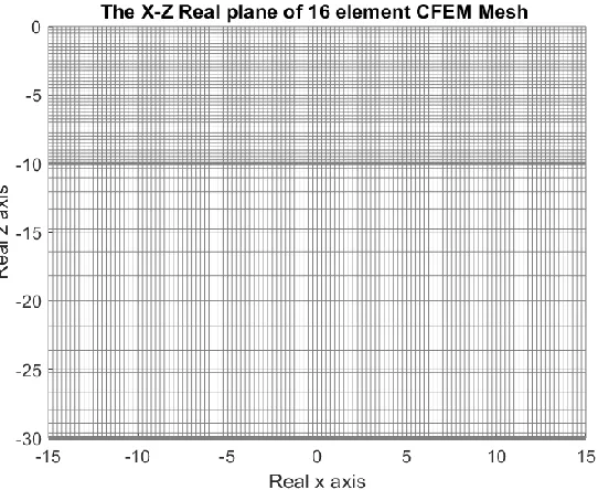
Figure 2-8 Real plane of the discretized soil domain ... 22
Figure 2-9 Bending of mesh into complex plane ... 23
Figure 3-1 1D solution in the far field ... 24
Figure 3-2 2D/3D modeling for the near field ... 25
Figure 3-3 Schematic of the general model problem ... 26
Figure 3-4 Exploded view of a 3D domain showing stresses on the boundaries with free top surface ... 31
Figure 3-5 Illustration of consistent deconvolution ... 35
Figure 3-6 Schematic for scattering formalism ... 36
Figure 3-7 Domain depicting the interior ... 36
Figure 3-8 Scattered wave field in the exterior ... 37
Figure 4-1 A Log plot of the convergence ... 42
Figure 4-2 Schematic of the three layered soil profile ... 44
Figure 4-3 Amplification response plot ... 45
Figure 4-4 Converged FE and CFE plots for a target of 1% relative error ... 46
Figure 4-5 Plane strain response of structure ... 47
Figure 4-6 Five layered soil site - PS vs APS response ... 49
Figure 4-7 Antiplane shear - CFE performance ... 50
Figure 4-8 Plane strain - CFE performance ... 51
Figure 7-1 Domain depicting the exterior and interior separation ... 57
Figure 7-2 Incident wave field in scatter free exterior ... 58
1 INTRODUCTION
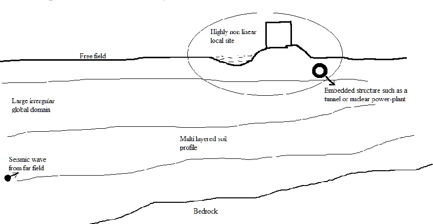
Modeling of problems where a small scale system is present and interacting with a much larger system forms a broad class of two-scale problems. The size difference and complexity of interaction entails that such systems do not easily conform to simplistic methods of analysis. In the context of dynamic soil-structure interaction (SSI) modeling subjected to earthquakes, the layered geotechnical site forms the global system. On the other hand, the system of interest, such as a building or a tunnel, with nearby irregularities forms the smaller scale local system. The goal of this thesis is to address this problem of two-scale soil structure interaction in order to estimate the structural response with an inherent assumption of the seismic source being far away from the system.
1.1 Review of existing methods
Loma Prieta earthquakes were crucial in establishing the significance of local site effects on the soil response as illustrated in (4).
To account for the SSI effects, methods involving superposition of responses were developed. First the site response is obtained which is then used to obtain the structural response. In this context, 1D and/or 2D site response estimation techniques serve as the starting point for SSI analysis (1). These involve developing synthetic seismograms to predict ground motion or using recorded free field ground motion which can then be deconvoluted to obtain the entire site response. For example, reference (5) provides a blind deconvolution method to obtain the site response characteristics. Other studies such as (6) and (7) compare different site response analysis methods as well as ways to obtain the fundamental period of a soil site consisting of multiple soil layers.
With this in mind, some approaches in SSI analysis include semi-analytical methods such as (13), but they apply to ground motions with the source near to the site. But this thesis deals with SSI analysis when the causative fault is far away from the site. Studies such as (14) highlight the differences in response when analyzing near-fault and far-fault SSI systems. In general finite-element based SSI analysis uses direct or sub-structure methods (1). Direct methods involve modeling the entire region along with the site and the causative fault. Using direct methods in 2D or 3D setting necessitates the need for significant computational effort to simulate the soil-structure interaction problem (e.g. (15)). For our case, when the earthquake originates at an unknown location far away from the site, and characterization of the propagation path is unknown, utilizing direct methods renders modeling the entire region infeasible.
An improvement over this, provided by (22), is the Domain Reduction Method (DRM), which restricts the problem to the local domain but requires an explicit boundary layer around that domain. The method proposed in (23) utilizes a procedure similar to DRM, but without the dependency on the boundary layer and instead uses a stiffness consistent traction in the formulation. However, it does not address the computational cost issue that enters due to the discretization of large soil layers. The importance of efficiently solving the soil-structure interaction problem is further highlighted in a 3D setting with embedded structures such as tunnels (see e.g. (24), (25)). To address issues of computational cost, a transformation based approach was suggested in (26). Hybrid-methods to reduce computational cost were also developed e.g. in (27) but they have increased complexity.
1.2 Response Estimation Away from the Source
One of the critical factors in seismic response estimation away from the source is that, due to unknown magnitude, directivity and properties of the seismic wave, there is a need to rely on ground motion records. Databases such as those provided by PEER and USGS, provide valuable starting points to assess the nature of earthquake occurring in the region. Many ground response estimation techniques utilize the recorded ground motions at the surface to arrive at bedrock motions using approaches such as deconvolution. We follow a similar approach in this thesis.
Specifically, we assume that we have the ground motion at the surface and the knowledge of the local site profile, i.e. the geometry and material properties that can be obtained using geologic soil profiling or other subsurface investigation technique.
1.3 Assumptions used in the model
For a soil structure system set far away from the source, the free field ground motion is obtained from recorded data and the spatial variation of ground motion in that region is lost. This implies that in the worst case, a local region has to rely on the recorded data obtained from just one seismogram. The incident wave then, has to be assumed to be only a function of depth and spatially invariant in other directions. Such an assumption can be justified by the fact that top soil layers are slower than the deeper layers making the earthquake waves bend vertically as they enter the top layers (Snell’s law).
Yet another assumption inherent in this analysis is that of a linear, unbounded global domain. The geotechnical site is assumed to be a horizontally layered, semi-infinite half-space that is linear and homogenous in the direction of unboundedness.
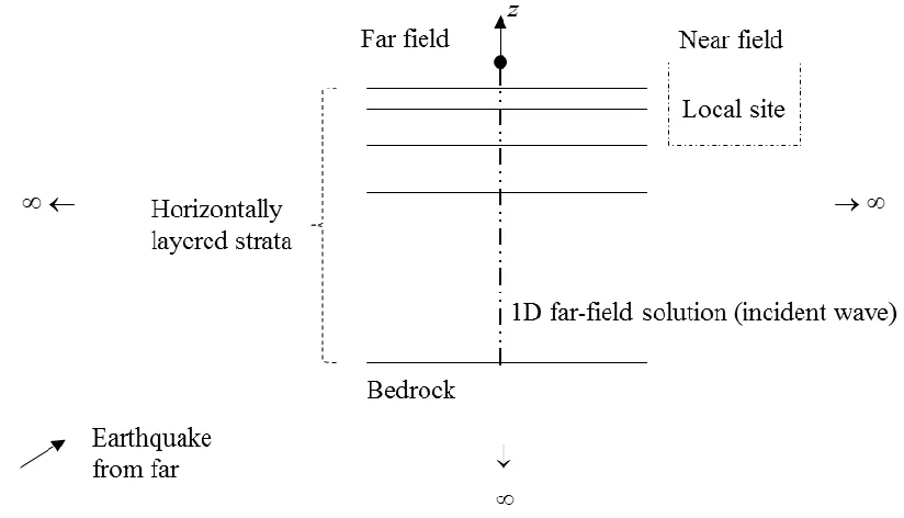
1.4 Schematic of the soil-structure problem
i
z
x
Figure 1-3 Schematic of the reduced model problem
The goal is to determine the response of the soil structure system shown in Figure 1-3. The governing equations for anti-plane shear are given; plane strain equations are similar, albeit more complicated. In the interior i,
2 .
u u
G G u f
x x z z
(1.1.1)
Traction on the free surface is given by the homogenous Neumann boundary condition,
0.
u
G
n (1.1.2)
Radiation boundary condition is applicable in the exterior. 1.4.1 Problem statement:
The focus of this thesis is to provide an efficient way to solve for the responses, in the frequency domain of a 2D/3D soil structure system set far away from the source, subjected to vertically propagating shear waves, where a non-linear local site with the structure of interest interacts with the surrounding global site that is assumed linear, horizontally stratified and homogenous in the direction of unboundedness. While the method developed here can be extended to three-dimensional settings, the scope of the thesis is limited to two-dimensional settings, i.e. anti-plane shear and plane strain.
1.5 Issues with existing approaches – computational cost
2 PRELIMINARIES
This chapter illustrates three key ideas that will be used in the proposed solution methodology. 1) The Crank-Nicolson (CN) method
2) Perfectly Matched Discrete Layers (PMDL) 3) Complex Finite Elements (CFEM)
The concepts are presented in a stand-alone fashion in this chapter to aid in understanding of the overall formulation presented in the next chapter.
2.1 The Crank Nicolson Method
For a one-dimensional partial differential equation of the form,
z ,z
p
F (2.1.1)
the Crank-Nicolson finite difference approximation takes the form
1
1 1
, 2
n n
n n
z z
z
p p
F F (2.1.2)
where p and F are vector field variables and z the element length.
2.1.1 Crank Nicolson Method for 1D Wave Propagation
Figure 2-1 Vertically propagating 1D shear wave The governing differential equation can be written as:
22
2 z 0,
u
k u
z
(2.1.3)
0 0, z u G z
(2.1.4)
where, . z s k c
(2.1.5)
From the stress-strain constitutive equations, we have:
,
u G
z
(2.1.6)
where, u is the displacement wave field and is the shear stress. Substituting (2.1.6) in (2.1.3) gives,
2 0. zG k u
z
(2.1.7)
Rewriting (2.1.6) gives,
0. u z G
(2.1.8)
2 1 0 0 . 0 0 z u u G z G k (2.1.9)This is similar to Equation (2.1.1),
0,
z
p Ap (2.1.10)
where u
p and
2 1 0 . 0 z G G k A (2.1.11)
Using Crank-Nicolson method in Equation (2.1.10), we have, 1 1 1 . 2 n n n n z p p
A p p (2.1.12)
Rewriting this equation provides,
1
1 1 1 1
. 2 2 n n z z
I2 A p I2 A p (2.1.13)
This is the Crank-Nicolson propagator equation as it facilitates the propagation of the vector
p from zz0 to z zn1.
0 0 0 u
p is the initial value specified at z z0, and recursive application of Equation (2.1.13)
2.1.2 Crank Nicolson Method for 2D wave propagation
When the waves propagate obliquely, the formalism described above would still be valid, due to Snell’s law that states that the horizontal wavenumber is invariant through the depth. Thus, the wave-field can be split into multiple harmonics in the x direction, and Crank-Nicolson method is applicable after performing Fourier transform in the x direction. The associated equations are summarized below.
For in-plane waves with angular frequency, Lamé constants and , density and horizontal wavenumber kx, when written in first order form gives:
0,
z
p Ap (2.1.14)
where, x z xz zz u u
p is a function of
z,
, and A is given by,
2 2 2 2 1 0 0 1 0 02 2 .
4 0 0 2 2 0 0 x x x x x ik ik k ik ik
A (2.1.15)
The marching equation takes the form,
1
1 1 1 1
. 2 2 n n z z
After computing pat any depth, the remaining stress component, namely xx can be determined using the equation,
2
1
4 .
2
xx zz ik ux
(2.1.17)
2.1.3 Crank Nicolson Method for SSI Problem
The Crank-Nicolson method can be used as a method of deconvolution of free field motion to obtain the ground motion throughout the depth. Deconvolution is the process of using Initial values of stresses and displacements at the free field and the stiffness of the soil layer to obtain the ground motion at a depth. In a discrete system, this involves obtaining the propagator matrix and marching through the depth to obtain the deconvoluted field values. The Crank Nicolson method is one such propagator method. The effectiveness of the CN method in this context is further discussed in Section 3.5.2.
2.2 Perfectly Matched Discrete Layers (PMDL)
2.2.1 The idea behind PMDL
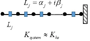
Figure 2-2 presents the basic summary of how PMDL approximates the half-space stiffness, in the simpler 1D setting. Figure a) denotes the continuous half-space with an exact stiffness
hs
K . Adding a single element to the half space with regular integration (say two point) results in Ksystem that does not equal the exact half-space stiffness, due to finite element discretization error. However, utilizing midpoint integration to evaluate the system matrices eliminates the discretization error and the resulting system stiffness exactly equals the half-space stiffness (29). The crucial point to note is that the half-space impedance is recovered irrespective of element length. The next step is to recursively replace the unbounded domain with midpoint-integrated elements. To keep the system finite, truncation is introduced after some elements. Due to truncation an error is introduced into the system stiffness. The length of the elements (PMDL parameters) are chosen so as to minimize this error. It turns out that in the context of wave propagation, reducing the error requires complex element lengths, similar to the celebrated method of perfectly matched layers (PML), (see (30), (31)). A specific approach to choose the PMDL element lengths is presented in (29) and summarized below:
2 , j j ic L
(2.2.1)
where
1
, :1 .cos 2 j
c
c j n
j n (2.2.2) j
L : Length of the jth element n : Number of PMDL elements used
2.2.2 PMDL for 2D mesh
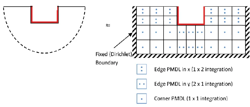
For a 2D domain, the PMDL mesh for the edges is the product of regular FEM discretization along the boundary and 1D PMDL discretization perpendicular to the boundary. On the other hand, at the corners, the PMDL mesh consists of tensor product of two 1D PMDL discretization perpendicular to each of the two edges meeting at the corner (see (29)). A typical 2D mesh is shwon in Figure 2-3.
Figure 2-3 PMDL approximation of exterior in 2D along with integration points (23)
2.2.3 PMDL for the SSI problem
The reduced problem of soil structure interaction consists of horizontally stratified medium with the outer domain being homogenous and unbounded for each layer in the horizontal direction and a half-space of bedrock extending infinitely below.
2.3 Complex-Length Finite Element Method
Complex-length Finite Element Method (CFEM) is a method to obtain the response at select localized regions, whereby the discretization along with nature of integration is modified so as to have exponential convergence at preselected points. In the case of layered subdomains, usage of CFEM inside the layer results in exponential convergence at the layer boundaries. While further details can be found in (33), a brief summary is given in the rest of the section. 2.3.1 Summary of CFEM
1) The mesh is bent into complex plane with specific lengths that are in complex conjugate pairs. Few complex finite elements are sufficient to achieve a high degree of accuracy. The choice of lengths are presented in Section 2.3.3
2) The elements are mid-point integrated along the direction of complex mesh bending.
Figure 2-4 Illustration of FEM vs CFEM - Mesh Bending (34) The key advantages are:
2) The lengths of the CFEM elements scale with the length of the layer and are independent of the domain properties or the frequency (as in contrast with PMDL). It must be pointed out that we do not obtain the response inside the layer modeled with CFEM, which is the price we pay for obtaining exponential convergence at the layer boundaries. 2.3.2 The idea behind CFEM
For a 1D Helmholtz equation of the form 2
2
2 0, [0, ],
u
u x L
x
(2.2.3)
where denotes the temporal frequency and u is the displacement. The exact stiffness or
the Dirichlet-to-Neumann (DtN) map
0, ( / ) 0,
x L x L
u du dx is given by,
exact cosh 1
. 1 cosh sinh i L i i L i L
K (2.2.4)
The discretization is such that, with mid-point integration and specially chosen complex valued lengths, for the Dirichlet-to-Neumann (DtN) map exponential convergence is achieved at the surface edges at the expense of solution accuracy in the interior.
2.3.3 Choice of CFE element lengths
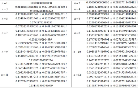
If Lj is element size and L the domain size, we can obtain j 2 j
L
L x where xj are the roots of
the nth degree polynomial given by,
2
!n n j
For lengths other than unity the values just scale. Illustrated below is a table of element lengths vs number of CFE elements used in a layer.
Figure 2-5 A table of element lengths with number of CFE elements used
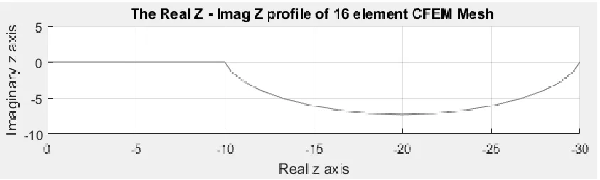
2.3.4 CFEM for SSI problem
In the context of soil-structure interaction (say for a 2D domain) where the soil layers are horizontally stratified and unbounded, we can employ CFEM in the vertical direction for the soil layers that do not contain the structure of interest because,
2) We are interested in obtaining the effects of the soil layers on the structure and domain of interest and not the solution in the soil layers themselves.
Consider an example domain consisting of two soil layers (Figure 2-6) where the top layer contains an embedded structure (e.g. a tunnel).
Figure 2-6 Example of soil domain to be discretized
Figure 2-9 Bending of mesh into complex plane
3 PROPOSED APPROACH
The first step is to divide the region into near and far field regions. The near field encompasses the structure and surrounding features which can be non-linear, while the rest of the domain (far field) is linear. The ground motion in the far field is developed from the free-field solution, which is invariant in the horizontal directions but depends on the depth, necessitating a 1D solution procedure (Figure 3-1).
Figure 3-1 1D solution in the far field
The same vertical discretization (along with CFE) is used in the far field to ensure consistent transfer of information between far-field and near-field models. Note that this is applicable for both vertically and obliquely propagating waves. Fourier transform in the horizontal direction is used for the latter case as described in Section 2.1.2; such problems are out of the scope of the present work.
Figure 3-2 2D/3D modeling for the near field
With respect to coupling the far-field and near-field models, due to the complex effects arising from the scattering in the near field, a scattering formalism is employed as described later in this section.
To summarize the main ingredients,
2) A 2D/3D near field system is used just for the reduced local domain, along with PMDL to mimic the exterior.
3) CFEM is used in the vertical direction with discretization consistent with near and far-field which makes the system computationally efficient.
4) A scattering formalism is employed to couple the near-field and far-field models. Below are the details of the stepwise development of the entire approach.
3.1 The continuous problem
Consider a horizontally layered 3D domain that encompasses the near and far field regions. Earthquake excitation is incident from outside of this region.
Figure 3-3 Schematic of the general model problem
2
0,
xx yx zx x
xy yy zy y
xz yz zz z
u u
x y z
u (3.1.1)
where u is the displacement, , are the stresses, is the density and the angular frequency.
Each of the three equations can be written as, 2
0, u
σ (3.1.2)
where, 1 2 3 .
σ (3.1.3)
u and the three components of σ depend upon the direction of equilibrium Equation (3.1.1) . For example, in the x direction, u ux and σ becomes,
. xx x yx zx
σ (3.1.4)
Using the weak formulation, Equation (3.1.2) becomes,
2
0,
u u d
σ (3.1.5)where uu.
3.2 Integration by parts in z followed by Semi-discretization in z direction
where the computational domain (near and far field) has a depth of H in the negative z
direction.
Integration by parts in z, i.e.,
3 3 3 .
u
u dz u dz
z z
(3.2.2)Equation (3.2.1) can then be rewritten as,
0 0
0 2
1 2 3 H 3 0.
H H
u
u u dz u dz
x y z
(3.2.3)Semi-discretization is performed in the z direction for both the local and global domain. PMDL in the z direction is also employed. The following approximation is used for the displacement field.
1 , , , , , , . n T i i iu z u x y z z x y z
Φ U (3.2.4)Here Φ
z is the basis function vector and U
x y z, , ,
the nodal degrees of freedom vector. Galerkin method is employed in this approximation where the test function takes the same form as the solution given by,
1 , , , , , , . n T T i i iu z u x y z z x y z
Φ U U Φ (3.2.5)The stress term correspondingly takes the form,
1 , , , , , , . n T i i iz x y z w z x y z w
Φ Σ (3.2.6)Using these semi-discretization approximations in (3.2.3) we have,
0 0
0 2
1 2 3 3 0.
T T T T T T
z H H H dz dz x y
U Φ Φ Σ Φ Σ Φ U ΦΦ Σ Φ Φ Σ
21 2 3 0,
x y
A Σ Σ U B Σ (3.2.8)
Where, 0 , T H dz
A ΦΦ (3.2.9)
0. T T z z H H dz
B ΦΦ Φ Φ (3.2.10)
Both the (2D/3D) near-field model and the 1D far-field model make use of the same discretization (with Φ
z as the basis function vector) in the z direction.3.3 Near field: Integration by parts in x y, directions
For the near field region, regular finite elements are used in the x (and y) directions. Thus weak form of the semi-discrete form of the governing equation (3.2.8) is obtained by appropriate integration by parts in x (and y) directions.
Integration by parts of the first term of (3.2.8) w.r.t x yields,
/ 2 / 2
1 1 1
/ 2 / 2
.
L L
L L
u
u dx u dx
x x
A Σ AΣ
AΣ (3.2.11)Integration by parts in the y direction, for the second term of (3.2.8) takes a similar form:
B/ 2 B/ 2
2 2 2
/ 2 / 2
,
B B
u
u dy u dy
y y
A Σ AΣ
AΣ (3.2.12)where the domain in x direction is assumed to span a length of L from 2
L
to 2
L
The system is then discretized in x and y directions using standard FEM along with PMDL.
3.4 Boundary Tractions
The traction at the boundaries arises from evaluating the
AΣi
term in each of the equations (3.2.11) and (3.2.12). While the former gives the traction on the x boundaries the latter provides the tractions on the y boundaries.Without loss of generality, let 1 2
Σ be the stresses for an element with two nodes in the
vertical direction. Using linear elements in z direction with midpoint integration results in: 0 1 1 , 1 1 4 T z z dz
A ΦΦ (3.3.1)
where z is the height of the element under consideration.
For a given element, the nodal forces Pi take the form,
1 1 2 2 1 1 . 1 1 4 i element P z P
AΣ (3.3.2)
If there are n1 nodes and corresponding values of stresses such that,
1 2 1 , n
Σ (3.3.3)
1 2
1
2 3
1 2
1 2
2 3 3 4
2 3
4
4 4 .
4 4
z
z z
z z
P (3.3.4)
This can be done for all three directions with each boundary consisting of three stress components as illustrated in Figure 3-4.
3.5 Solution in the Exterior: Crank-Nicolson Method Consistent with
Semi-discretization
The traction specification outlined in Section 3.4 makes use of the stresses at the nodes along the vertical direction to compute the traction acting on a boundary. Thus it is crucial to arrive at the correct values of displacements and stresses at the nodes, especially when unconventional discretization such as CFEM is used.
One way to ensure consistency would be to use the FE stiffness of the layer for the exterior solution. But the exterior problem is not a boundary value problem but an initial value problem (deconvolution) which requires a propagator matrix approach in the z direction. As already described one such deconvolution would be the Crank-Nicolson method. The displacement and stresses in the vertical direction are computed by marching in space in the vertical z
direction, following (2.1.13):
1
1 1 1 1
, 2 2 n n z z
I2 A p I2 A p (3.4.1)
where u
p . The initial value at the free field is prescribed using 0 0 0 u
p obtained from
the free field ground motion. For a free surface,0 0.
3.5.1 CFEM in the Interior
No excitation occurs inside the layers and hence in the z direction CFEM is employed in the interior for the layers that do not contain the structure of interest. The model schematic is illustrated in Section 2.3.4. The mesh in the vertical direction bent into complex plane, with linear interpolation and midpoint integration utilized in that direction (Section 2.3).
3.5.2 Consistent CFEM in the exterior (Crank Nicolson method with consistent complex valued steps)
If only FEM were used in the z direction, in the limit, the discrete approximation converges to the continuous case. However, the usage of CFEM implies that the developed stresses and displacement at the nodes must be consistent and equivalent with the modified mesh discretization.
In the z direction, the weak form of the equation (3.2.1) reduces to 2
.
u
u G u dz
z z
(3.4.2)Using Galerkin approximation with semi-discretization, this is of the form .
T T
z z dz dz
Φ Φ
ΦΦ U Σ (3.4.3)Evaluating the stiffness relation for a single element in the vertical direction with linear shape functions and mid-point integration we have,
1 1 1 1
1 z u
Using
, the above equation can be written in the propagator matrix form as,
2 1 2 1
2 1 2 1
0 2 , 0 2 i i
u u u u
z z (3.4.5)
which can be written as
. mid i
mid
u u
z
P (3.4.6)
This is equivalent to the Crank Nicolson propagator matrix formulation (see Section 2.1). This link provides the crucial basis for transferring information from the far-field deconvolution model to the near field interior domain.
Figure 3-5 Illustration of consistent deconvolution
3.6 Solution in the Interior: Scattering Formalism
Figure 3-6 Schematic for scattering formalism
The goal now is to solve for the soil-structure interaction occurring in the interior region. Let the final solution for displacement be denoted by u. The displacements obtained through the Crank Nicolson approach (solution in the exterior) gives the solution in the far-field, i.e. the incident wave-field denoted byuI. The consistent tractions prescribed on the boundary, as obtained from Section 3.4, be noted by P.
For sake of illustration, a 1-D diagram (Figure 3-7) is used to depict the entire system, but the formulations are generic and hold true for 2D and 3D settings. The exterior, boundary and interior are denoted by subscripts e b, and i respectively.
From Figure 3-7, the interior equilibrium equations can be written as,
,
ii ib i i
bi bb b b
K K u P
K K u P (3.5.1)
whereK refers to the dynamic stiffness matrix.
One way to solve the system would be to split the solution into incident and scattered wave fields. Let the scattered displacement be denoted by uS and corresponding traction by S
P . The scattered wave field satisfies the radiation boundary condition. This means that the waves must be purely outgoing and the exterior mesh modeled cannot have any incident excitation
Figure 3-8 Scattered wave field in the exterior The equation for the scattered wave field now becomes,
. 0
S S
bb be b b
S e eb ee u P K K u
K K (3.5.2)
Using dynamic condensation we have,
1.
S S
bb
b be ee eb b
P K K K K u (3.5.3)
Using I S
i i i
u u u and I S
b b b
u u u and I S
b b b
P P P we have,
1 .I S
ii ib
i ii ib i i
I I S
bb
b bi bb b bi be ee eb b
K K
P K K u u
The left hand side of (3.5.4) can be explicitly calculated from the deconvoluted incident wave field, and applied as tractions to determine S
u .
While the scattered formalism described above applies to linear systems, SSI problems involve non-linear interiors, necessitating a formulation in terms of total displacement. Thus, rewriting
(3.5.2) with S I
b b b
P P P and S I
b b b
u u u we have,
.
I I
bb be b b b bb b
S I
e
eb ee eb b
u
K K P P K u
u
K K K u (3.5.5)
Note that in the second equation of (3.5.5), the exterior denoted by e can be further split into 1
e (first layer of exterior nodes) and er(rest of the exterior nodes).
Assembling (3.5.5) with (3.5.1) and setting Pi 0, the final formulation takes the form,
1
1
1 1 1 1 1
1
0 0 0
0
. 0
0 0 0
r
r
r r r
ii ib i
I I
bb b bb
bi bb be b b
I e
e b e e e e e b b
e e e e e
K K u
u
K K K K P K u
u
K K K K u
u
K K
(3.5.6)
The only unknowns in the right hand side of equation(3.5.6) are ubI and the effective forces I
b
P , acting on the boundary nodes, which are computed as discussed in Section 3.4.
3.7 Summary of the procedure
2) Apart from the layers containing the structure of interest, CFEM is used for the layers in vertical direction.
3) The exterior is efficiently modeled using PMDL.
4) The stresses τbI and displacements ubI are calculated at the boundary nodes from the incident wave field. This is done by consistent CN deconvolution of free field ground motion.
5) Tractions are specified at the boundary nodes, consistent with CFEM.
6) The system is solved for the displacement response using the scattering formalism.
3.8 Application to SSI
3.8.1 Anti-plane shear
Anti-plane shear deformation occurs in the form of vertically propagating shear horizontal (SH) waves. For a 2D domain in the xz plane, the incident wave would have a displacement component uy and a shear stress component zy(along with its complementary shearyz ). For this case, the incident wave field and the stresses are a function of only the depth (z). The traction in Equation (3.5.6) acts on the surface of the side boundaries and is of the form
uyx
3.8.2 Plane strain
Plane strain response arises out of incident waves that are vertically propagating shear vertical (SV) waves. In this case, for a 2D domain in the xz plane, the incident wave has a displacement component ux and a shear stress component xz (along with its complementary shearzx ). ux is a function of x , which implies that traction is present in the side boundaries. This is crucial, as it implies that the traction so obtained must be consistent with the CFEM used on the side boundaries. To this end, the traction specification developed earlier based on mid-point integration ensures that the traction specified at the nodes are correct and consistent with CFEM.
4 NUMERICAL EXAMPLES
4.1 Verification of the approach
To verify the developed methodology, vertically incident shear wave is input onto a homogenous soil half-space. The half space is devoid of any scatterer and has a global free field motion of unit amplitude in the y direction for the case of anti-plane shear and in x
direction for the case of plane strain.
For a given frequency and a soil of shear wave velocity cs the wavenumber of the incident
wave in the vertical (z) direction is s
l c
. Hence the incident wave is of the form cos
lzand invariant in x direction.
Figure 4-1 A Log plot of the convergence
4.2 Response amplification in Anti-plane shear
A structure with its base-mat resting on a three-layer soil is analyzed in anti-plane shear and compared with the response amplification of the same structure resting on homogenous soil half-spaces of different velocities. The structure is idealized as a rectangular domain with geometric and material properties shown in
Table 4-2, while the properties of soil layers are shown in Table 4-3.
Table 4-1 Structure dimensions and properties
Length 10 m
Height 20 m
G (shear modulus) 50 MPa
(Density) 2000 kg/m3
Table 4-2 Base-mat dimensions and properties
Length 15 m
Height 1.5 m embedded in soil
G (shear modulus) 10 GPa
(Density) 2500 kg/m3
Table 4-3 Soil layers
Depth in (m) Cs in m/s (Shear wave velocity)
in (kg/m3)
Layer 1 50 300 1800
Layer 2 150 500 1800
Layer 3 300 1000 1800
Bedrock Halfspace 4000 2700
Figure 4-2 Schematic of the three layered soil profile
distinct peaks are observed consistent with the existence of three distinct layers, but the overall effect has resulted in a decreased maximum amplification.
Figure 4-3 Amplification response plot 4.2.1 Performance of CFEM
Figure 4-4 Converged FE and CFE plots for a target of 1% relative error
Table 4-4 Performance comparison - FE vs CFE
Number of elements used in the vertical direction
Number of elements Extrapolating to 3D problem
Regular FE 120 1.2 million
Complex FE 18 180,000
4.3 Response amplification in plane strain
second. A closer look at the homogenous profile shows that the soils with higher shear wave velocity tend to have a greater amplification and at a time period lesser than that of lower velocity layers, which is expected and in agreement with the observation for the case of anti-plane shear. The amplification for multi-layered system is significantly different form that of homogenous soil profiles especially at higher frequencies. The sharp variations observed at higher frequency may be due to the presence of higher modes of vibration at larger frequencies and complex mode coupling that exists in plane strain.
4.4 Response amplification for Realistic Soil-Structure System
For this example, a soil profile similar to an actual site in Taiwan is used (35). The soil profile data was obtained from borehole measurements and the paper (35) provides the geometry and geotechnical characterization of the site. The same structure with base-mat is used on this new soil-profile and the response obtained for the case of plane-strain and anti-plane shear. A comparison of performance of the CFEM based approach is carried out against a full FEM model. The structure and base-mat properties are the same as in
Table 4-1 and
Table 4-2. The soil characteristics are given in Table 4-5. The amplification factors are shown in Figure 4-6.
Table 4-5 Soil properties for five-layer system
Layers Height in m Shear Modulus in MPa
1 20 90
2 5 115
3 6 65
4 7 160
5 11 65
6 Halfspace 43.2 GPa
Density: (For all the soil layers) 1960 kg/m3
Poisson’s ratio: (For all soil layers) 0.25
Figure 4-6 Five layered soil site - PS vs APS response
4.4.1 Performance Analysis: CFE vs FE - Example 2
Figure 4-7 and Figure 4-8 illustrate the fast convergence offered by CFEM, compared to slow algebraic convergence of FEM. The number of elements in the vertical direction required for CFEM is an order of magnitude less than FEM, while the error in CFEM is several orders of magnitude smaller, clearly illustrating the efficiency offered by CFEM.
5 SUMMARY AND CONCLUSIONS
6 REFERENCES
1. Kramer SL. Geotechnical earthquake engineering. Pearson Education India; 1996. 2. Aki K, Richards PG. Quantitative seismology. ; 2002.
3. Mylonakis G, Gazetas G. Seismic soil-structure interaction: beneficial or detrimental? J Earthquake Eng. 2000;4(03):277-301.
4. Seed RB, Dickenson SE, Mok CM. Recent lessons regarding seismic response analysis of soft and deep clay sites. In: Technical Report NCEER. US National Center for Earthquake Engineering Research (NCEER); 1992. p. 131-45.
5. Zerva A, Petropulu AP, Bard P. Blind deconvolution methodology for site-response evaluation exclusively from ground-surface seismic recordings. Soil Dyn Earthquake Eng. 1999;18(1):47-57.
6. Arslan H, Siyahi B. A comparative study on linear and nonlinear site response analysis. Environ Geol. 2006;50(8):1193-200.
7. Motazedian D, Banab KK, Hunter JA, Sivathayalan S, Crow H, Brooks G. Comparison of site periods derived from different evaluation methods. Bulletin of the Seismological Society of America. 2011;101(6):2942-54.
8. Stewart JP, Fenves GL, Seed RB. Seismic soil-structure interaction in buildings. I: Analytical methods. J Geotech Geoenviron Eng. 1999;125(1):26-37.
9. Safak E. Discrete-time analysis of seismic site amplification. J Eng Mech. 1995;121(7):801-9.
10. Venture NCJ. Soil-structure interaction for building structures. NIST GCR. 2012:12-917. 11. Bielak J, Xu J, Ghattas O. Earthquake ground motion and structural response in alluvial valleys. J Geotech Geoenviron Eng. 1999;125(5):413-23.
13. Hisada Y. An efficient method for computing Green's functions for a layered half-space with sources and receivers at close depths. Bulletin of the Seismological Society of America. 1994;84(5):1456-72.
14. Davoodi M, Sadjadi M, Goljahani P, Kamalian M. Effects of Near-Field and Far-Field Earthquakes on Seismic Response of SDOF System Considering Soil Structure Interaction. 15th World Conference on Earthquake Engineering. Lisbon, Portugal; ; 2012.
15. Bao H, Bielak J, Ghattas O, Kallivokas LF, O'Hallaron DR, Shewchuk JR, et al. Large-scale simulation of elastic wave propagation in heterogeneous media on parallel computers. Comput Methods Appl Mech Eng. 1998;152(1):85-102.
16. Wolf JP. Dynamic soil-structure interaction. Prentice Hall int.; 1985.
17. Lysmer J, Tabatabaie-Raissi M, Tajirian F, Vahdani S, Ostadan F. SASSI. System for Analysis of Soil Structure Interaction, UC Berkeley, Dept.of Civil Engineering, Berkeley, CA. 1983.
18. Nie J, Braverman J, Costantino M. Seismic Soil-Structure Interaction Analyses of a Deeply Embedded Model Reactor–SASSI Analyses. NIST GCR. 2013.
19. Jeremić B, Tafazzoli N, Ancheta T, Orbović N, Blahoianu A. Seismic behavior of NPP structures subjected to realistic 3D, inclined seismic motions, in variable layered soil/rock, on surface or embedded foundations. Nucl Eng Des. 2013;265:85-94.
20. Bolisetti C. Site Response, Soil-Structure Interaction and Structure-Soil-Structure Interaction for Performance Assessment of Buildings and Nuclear Structures. Technical Report MCEER-15-0002. 2014.
21. Ashrafi SA, Abruzzo J, Singh P, Vahdani S. Seismic Soil-Structure Interaction Analysis for the Transbay Transit Center in San Francisco–Methodology. 15th World Conference on Earthquake Engineering; ; 2012.
22. Bielak J, Loukakis K, Hisada Y, Yoshimura C. Domain reduction method for three-dimensional earthquake modeling in localized regions, Part I: Theory. Bulletin of the Seismological Society of America. 2003;93(2):817-24.
23. Guddati M, Savadatti S. Efficient and accurate domain-truncation techniques for seismic soil-structure interaction. Earthquakes and Structures. 2012;3(3_4):563-80.
25. Donikian R, Liu C, Liu Q, Clinch K. THREE-DIMENSIONAL SOIL-STRUCTURE INTERACTION ANALYSIS OF CUT-AND-COVER TUNNELS.
26. Humar JL, Bagchi A, Xia H. Frequency domain analysis of soil-structure interaction. Comput Struct. 1998;66(2):337-51.
27. Gupta S, Penzien J, Lin TW, Yeh CS. Three‐dimensional hybrid modelling of soil‐ structure interaction. Earthquake Eng Struct Dyn. 1982;10(1):69-87.
28. Guddati MN, Lim KW, Zahid MA. Perfectly matched discrete layers for unbounded domain modeling. Computational Methods for Acoustics Problem, Saxe-Coburg
Publications, Scotland. 2008:69-98.
29. Guddati MN, Lim K. Continued fraction absorbing boundary conditions for convex polygonal domains. Int J Numer Methods Eng. 2006;66(6):949-77.
30. Berenger J. A perfectly matched layer for the absorption of electromagnetic waves. Journal of computational physics. 1994;114(2):185-200.
31. Chew WC, Weedon WH. A 3D perfectly matched medium from modified Maxwell's equations with stretched coordinates. Microwave Opt Technol Lett. 1994;7(13):599-604. 32. Savadatti S, Guddati MN. Absorbing boundary conditions for scalar waves in anisotropic media. Part 1: Time harmonic modeling. Journal of Computational Physics.
2010;229(19):6696-714.
33. Guddati MN, Druskin V, Astaneh AV. Exponential Convergence through Linear Finite Element Discretization of Stratified Subdomains. arXiv preprint arXiv:1507.05038. 2015. 34. Vaziri Astaneh A, Guddati MN. Efficient computation of dispersion curves for
multilayered waveguides and half-spaces. Comput Methods Appl Mech Eng. 2016;300:27-46.
35. Amorosi A, Annamaria DL, Boldini D. ADVANCED NUMERICAL APPROACHES TO THE SEISMIC SOIL AND STRUCTURAL RESPONSE ANALYSES. Cambridge UK: ; 2015.
7.1 Appendix A - The link between DRM and SCM
The scattering formalism developed by (23, 32) and illustrated in Section 3.6, which has been extended to include CFEM layers will herein be referred to as Stiffness-Consistent Method or SCM in short (since the traction is consistent with the stiffness).
The Domain Reduction Method (DRM) is an alternate approach (22) to SCM. The basic idea of DRM involves calculating the effective forces in the nodes of the first band of elements outside the boundary. The approaches developed in this thesis can be combined with DRM used in place of SCM; in fact, this has been implemented and found to work well.
A comparison on the equations of the DRM and SCM formulations provides an interesting insight into the links between the two approaches. The general idea is that both the approaches essentially have the same basis, but approach the problem of obtaining effective forces in the local domain differently; this Appendix aims to illustrate this link.
Figure 7-1 Domain depicting the exterior and interior separation
,
ii ib i i
bi bb b b
K K u P
K K u P
for i. (6.1.1)
bb be b b
e e eb ee u P K K u P K K
, for e. (6.1.2)
Subscripts b denotes boundary, i for interior and e for exterior nodes. K refers to the dynamic stiffness while P refers to the force vector.
7.1.1 The DRM Approach
DRM employs the fact that Pe (forcing in the exterior) is the same as PeI (incident forcing in the exterior).
Figure 7-2 Incident wave field in scatter free exterior
Hence if there was just the global domain without any local features, the exterior e for the incident wave field, takes the following form:
.
I I
bb be b b
I e e eb ee u P K K u P K K
,
I I
e eb b ee e
P K u K u (6.1.4)
which when used in equation (6.1.2) leads to
.
bb be b b
I I
e eb b ee e
eb ee
u P
K K
u K u K u
K K
(6.1.5)
Using I S
e e e
u u u , equation (6.1.5) becomes,
, I
bb be b b be e
S I
e eb b
eb ee
u P K u
K K
u K u
K K
(6.1.6)
which when assembled with i equation (6.1.1) gives the full DRM formulation. 7.1.2 The SCM Approach
The key difference in SCM is that, instead of looking at scatter free incident wave field (6.1.3) SCM uses radiation boundary condition in the scattered exterior wave field. Due to radiation boundary condition, there is no forcing arising from the exterior. This provides the scattered wave field in the exterior as:
. 0
S S
bb be b b
S e eb ee u P K K u K K
(6.1.7)
Note that the second equation of (6.1.7) is the same as the second equation of (6.1.5) with I S
uu u . Rewriting (6.1.7) with S I
b b b
P P P and S I
b b b
u u u we have,
.
I I
bb be b b b bb b
S I
e
eb ee eb b
u
K K P P K u
u
K K K u
(6.1.8)
SCM proceeds to calculate I b
P from the tractions on the boundary. For example, for the case of anti-plane shear, PbIwould be of the form:
. I b I b uP G
n (6.1.9)
Assembling Equations (6.1.8) and (6.1.1) gives the full SCM formulation.
Comparing the SCM formulation in Equation (6.1.8) and the DRM formulation in Equation (6.1.6) we note that the difference is in the right hand side:
DRM: I
be e
K u
SCM: PbI KbbubI
The first Equation in (6.1.3) gives the equivalence that
I I I
bb
be e b b
K u P K u
(6.1.10)