Extensions of Global Sensitivity Analysis: Theory, Computation, and Applications.

(1)

ABSTRACT

HART, JOSEPH LEE. Extensions of Global Sensitivity Analysis: Theory, Computation, and Applications. (Under the direction of Pierre Gremaud.)

(2)

(3)

Extensions of Global Sensitivity Analysis: Theory, Computation, and Applications

by Joseph Lee Hart

A dissertation submitted to the Graduate Faculty of North Carolina State University

in partial fulfillment of the requirements for the Degree of

Doctor of Philosophy

Applied Mathematics

Raleigh, North Carolina

2018

APPROVED BY:

Ralph Smith Alen Alexanderian

Emil Constantinescu External Member

Brian Reich

(4)

DEDICATION

(5)

BIOGRAPHY

Joseph Lee Hart graduated with a Associate of Arts degree from Cape Fear Community College in July 2012 with membership in Phi Theta Kappa and Mu Alpha Sigma. He transferred to North Carolina State University where we graduated summa cum laude with a Batchelor of Sciences degree in Mathematics in May 2014.

(6)

ACKNOWLEDGEMENTS

I am grateful to my advisor Pierre Gremaud for all of the time and energy he invested in me. Throughout my graduate studies, Pierre has provided excellent advise, encouragement, ideas, and opportunities to support my research and professional development.

I am grateful to my internship mentors Julie Bessac, Emil Constantinescu, and Bart van Bloemen Waanders for the opportunities and support they provided.

I am grateful to Alen Alexanderian and Ralph Smith for the multitude of helpful conversations and useful feedback they have given me.

(7)

TABLE OF CONTENTS

LIST OF TABLES . . . vii

LIST OF FIGURES . . . .viii

Chapter 1 INTRODUCTION . . . 1

1.1 Motivation . . . 1

1.2 Review of Sobol’ indices . . . 2

1.2.1 Mathematical formulation . . . 2

1.2.2 Properties . . . 4

1.2.3 Estimation of Sobol’ indices . . . 4

1.3 Review of derivative-based global sensitivity measures . . . 6

1.4 Overview of other GSA methods . . . 7

1.5 Outline of the thesis . . . 8

1.6 Overview of the author’s work . . . 9

Chapter 2 SOBOL’ INDICES WITH DEPENDENT VARIABLES . . . 10

2.1 Introduction . . . 10

2.2 An approximation theoretic perspective of total Sobol’ indices . . . 12

2.3 Applying the approximation theoretic perspective for dimension reduction . . . . 15

2.4 Practical and computational considerations . . . 17

2.5 Illustrative examples . . . 18

2.5.1 A linear function . . . 18

2.5.2 A nonlinear function . . . 20

2.6 Conclusion . . . 21

Chapter 3 ROBUSTNESS OF SOBOL’ INDICES TO INPUT DISTRIBU-TION UNCERTAINTY . . . 22

3.2 Robustness of the Sobol’ index to PDF perturbations . . . 23

3.3 Robustness of the normalized total Sobol’ index to PDF perturbations . . . 29

3.4 Algorithmic description . . . 31

3.5 Numerical results . . . 34

3.5.1 Synthetic example to demonstrate convergence in samples . . . 34

3.5.2 Synthetic example to demonstrate the normalized total Sobol’ indices . . 35

3.5.3 Lorenz system . . . 35

Chapter 4 SOBOL’ INDICES FOR STOCHASTIC MODELS . . . 41

4.2 Formulation and method . . . 44

4.3.1 The stochastic g-function . . . 47

(8)

Chapter 5 DERIVATIVE-BASED GSA FOR STATISTICAL MODEL PA-RAMETERS . . . 56

5.2 Preliminaries . . . 57

5.3 Computing sensitivities . . . 60

5.3.1 Preprocessing stage . . . 60

5.3.2 Sampling stage . . . 61

5.3.3 post-processing stage . . . 66

5.3.4 Summary of the method . . . 69

5.4.1 Synthetic test problem . . . 70

5.4.2 Analysis of a space-time Gaussian process . . . 72

Chapter 6 DERIVATIVE-BASED GSA FOR PDE-CONSTRAINED OPTI-MIZATION. . . 82

6.2 Overview of sensitivity analysis for PDE-constrained optimization . . . 83

6.2.1 Control problem formulation . . . 83

6.2.2 Sensitivity formulation . . . 84

6.2.3 Discretization . . . 86

6.2.4 An illustrative example . . . 88

6.3 Overview of extensions and contributions . . . 89

6.4 Proposed reformulation . . . 90

6.5 Overview of randomized linear algebra . . . 91

6.6 Software implementation . . . 94

6.6.1 ApplyingMXh and MUh . . . 95

6.6.2 Applying Π . . . 95

6.6.3 Applying_K−1 _{. . . 95}

6.6.4 Applying_B . . . 95

6.7 Formulation of global sensitivity indices . . . 96

6.8 Computation, visualization, and interpretation of sensitivities . . . 98

Chapter 7 CONCLUSION . . . .107

(9)

LIST OF TABLES

Table 2.1 Total Sobol’ indices of (2.9) for variablesX1,X2, and (X1, X2) whenρ= 1. 20 Table 3.1 Marginal distribution for uncertain variables in Lorenz system Case 1. The

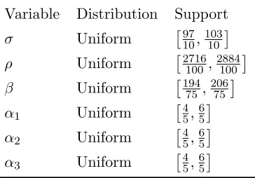
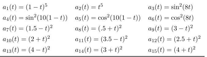
means of σ,ρ, and β are the nominal values in [84]. . . 37 Table 4.1 Expressions of the parametersak,k= 1, . . . ,15, for the stochastic g-function

(10)

LIST OF FIGURES

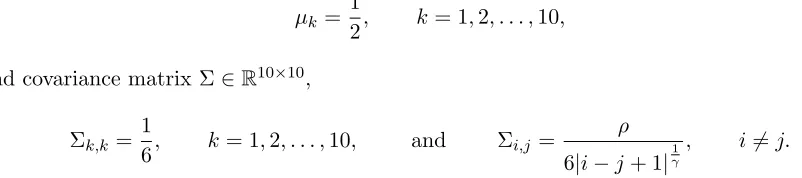
Figure 2.1 Total Sobol’ indices for (2.9) with increasing correlation strength as ρ varies from 0 to 1. . . 19 Figure 2.2 Sobol’ indexT7,8,9,10and approximation errorδ7,8,9,10for (2.10) asρ varies

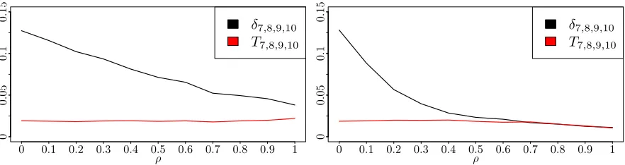
from 0 to 1. Left: γ = 1; right:γ = 6. . . 21 Figure 3.1 Convergence of the total Sobol’ index for variable X1 as the number

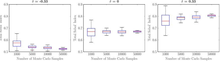
of Monte Carlo samples vary. Left: perturbed total Sobol’ index with δ =₋.33, center: nominal total Sobol’ index, right: perturbed total Sobol’ index with δ=.33. . . 35 Figure 3.2 Total Sobol’ indices for (3.9), the height of each bar indicates the total

Sobol’ index. The blue bars indicate the nominal total Sobol’ indices; the cyan and yellow bars indicate the total Sobol’ indices when the PDF of X was perturbed in extreme cases; cyan: the largest absolute change; yellow: the largest relative change. . . 36 Figure 3.3 Total Sobol’ indices for the Lorenz System Case 1 example, the height

of each bar indicates the total Sobol’ index. The blue bars indicate the nominal total Sobol’ indices; the cyan and yellow bars indicate the total Sobol’ indices when the PDF of X was perturbed in extreme cases; cyan: the largest absolute change; yellow: the largest relative change. . . 37 Figure 3.4 Total Sobol’ indices for the Lorenz System Case 2 example, the height

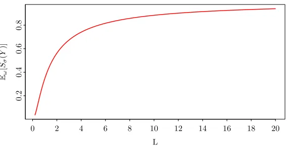
of each bar indicates the total Sobol’ index. The blue bars indicate the nominal total Sobol’ indices; the cyan and yellow bars indicate the total Sobol’ indices when the PDF of X was perturbed in extreme cases; cyan: the largest absolute change; yellow: the largest relative change. The left and right panel correspond to generating the partition by training a Regression Tree to: predict f with a minimum ofL samples per hyperrectangle (left) and predict f with a minimum of 4L samples per hyperrectangle, followed by additional partitioning of α3 (right). . . 39 Figure 4.1 Expected first order Sobol’ index of Y from (4.2) with respect to the

uncertain variable σ as a function ofL. . . 43 Figure 4.2 Convergence of the expected Sobol’ indices for the stochastic g-function

(11)

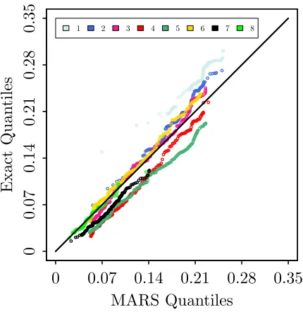
Figure 4.4 Convergence in distribution of the Sobol’ indices for the g-function (4.7). Top row;S1, index with the largest expectation; bottom row:S3, index with the largest variance. Left: heat map of the histograms as the surrogate sampling sizenvaries. Each vertical slice is a histogram for a fixedn; right: comparison of the “exact” (see text) and approximation distributions using n= 1000. . . 50 Figure 4.5 QQ plot of the Sobol’ indices of the eight most important variables. Lying

above or below the line indicates being biased high or low respectively. . . 51 Figure 4.6 Genetic oscillator: four realizations of the evolution of the complex C. . . 53 Figure 4.7 Evolution of the Sobol’ indices for the genetic oscillator. Left: expectation

of the Sobol’ indices. Each row corresponds to a specific reaction rate. Top right: time evolution of the expectation of the Sobol’ indices for the two most important reaction rates. Bottom right: time evolution of the histogram of the Sobol’ index of δR. Each vertical slice is a histogram for the Sobol’ index of δR at a given time. . . 54 Figure 5.1 Iteration history for parameter β1. Each frame corresponds to an

indepen-dent chain. . . 71 Figure 5.2 Sensitivity indices (left) and Pearson correlation coefficients of the

param-eters (right) for the synthetic test problem. . . 72 Figure 5.3 Sensitivity index perturbations for the synthetic test problem. Each line

corresponds to a given parameter. . . 72 Figure 5.4 Sensitivity indices for YNWP. The five colors represent the sensitivity

indices computed from each of the five chains. . . 75 Figure 5.5 Sensitivity index perturbations forYNWP. Each line corresponds to a given

parameter. . . 76 Figure 5.6 Pearson correlation coefficients for the parameters of YNWP. . . 77 Figure 5.7 Sensitivity indices for YObs|YNWP. The five colors represent the sensitivity

indices computed from each of the five chains. . . 78 Figure 5.8 Sensitivity index perturbations for YObs|YNWP. Each line corresponds to a

given parameter. . . 78 Figure 5.9 Pearson correlation coefficients for the parameters of YObs|YNWP. . . 79 Figure 5.10 Left: energy scores for each of the 14 days being predicted; right: root

mean square error for each of the 11 spatial locations being predicted. The full model is red and the reduced model is black. . . 80 Figure 5.11 Predictions using the full model (left) and reduced model (right) for 6

days at a fixed spatial location. The red curve is the observed wind speed and the grey curves are 1000 simulations generated from each model. . . . 80

(12)

Figure 6.3 Uncontrolled (left) and controlled (right) velocity field. . . 102 Figure 6.4 Control solutions for (6.16) corresponding to 20 different parameter

sam-ples. The left and right panels are the controllers on the left and right boundaries, respectively. Each curve is a control solution for a given parameter sample. . . 103 Figure 6.5 Leading 4 singular values of Dat 20 different parameter samples. Each

vertical slice corresponds to the leading 4 singular values for a fixed sample.103 Figure 6.6 Parameter sensitivities (6.15) for the 153 uncertain parameters in (6.16).

The 20 circles in each vertical slice indicates the sensitivity index for a fixed parameter as it varies over the 20 parameter samples. The repeating color scheme indicates the grouping of parameters as they correspond to sine and cosine components of each boundary condition. . . 104 Figure 6.7 First two singular vectors uk,k = 1,2, of D, i.e. Dxk = σkuk. The top

(13)

CHAPTER

1 INTRODUCTION

1.1 Motivation

Mathematical models and computer simulations are ubiquitous in engineering and scientific disciplines. Various systems and processes may be represented by mathematical models such as differential equations, interacting particles, or algebraic equations. These models are used to design structures, make policy decisions, and influence the development of systems in many spheres of society. However, models typically involve variables (or parameters) which are uncertain. These variables come in a variety of forms such as, but not limited to, chemical, material, or mechanical properties, electrical capacitance or resistance, or atmospheric conditions. They may appear as coefficients or boundary conditions in differential equations, parameters defining the simulation of dynamics, or algebraic expressions used to couple states in a system, to name a few. In all of these cases a user is seeking to utilize a mathematical model for scientific insight, design, or decision making, but is limited by uncertainties in the input variables of the model.

A mathematical abstraction of this is to represent uncertain quantities as random variables and the mathematical model as a function with these random variables as inputs. Global sensitivity analysis (GSA) aims to quantify the relative importance of these input variables on the output of the function. Such analysis facilitates, among other things,

(14)

• direction for model development,

• design of experiments and data acquisition,

• engineering risk adverse systems,

• reducing the number of uncertain variables to facilitate further analysis.

In some applications, GSA may not be tractable (or necessary) so practitioners use local sensitivity analysis (LSA) instead. The idea of LSA is to measure the influence of uncertain quantities at some nominal value rather than considering them as random variables. A basic example of this is to use the gradient of a function evaluated at a nominal point to rank the importance of the variables. This thesis focuses on GSA, the reader is directed to [59], and references therein, for a broader introduction to sensitivity analysis (GSA and LSA).

In practice, there are many tools for performing GSA, each of which has its own benefits and challenges. Different goals, model properties, types of uncertain variables, and quantities of interest (QoI) mandate different approaches to GSA. This thesis considers five problems where particular challenges prompted interest in developing a GSA tool relevant to the problem. This chapter introduces two commonly used GSA tools, the Sobol’ indices and derivative-based global sensitivity measures, and references other methods of interest that are not immediately relevant to this thesis. The subsequent five chapters present the author’s work on five different problems; the final chapter leaves concluding remarks and highlights other problems for future work.

1.2 Review of Sobol’ indices

This section reviews the Sobol’ indices. The references [57, 96, 104] are noted as useful resources.

1.2.1 Mathematical formulation

Let (Θ,F, ν) be a probability space with sample space Θ,σ-algebraF, and probability measureν. LetX: Θ_{→ X}, _X =_X1× X2× · · · × Xp ⊆Rp, be a random vector with distribution function Φ, and (_X,FX, νX) be the probability space induced byX, i.e.X is the image ofX,FXis the Borel

σ-algebra, andνX is the measure corresponding to the law ofX. Each setXi ⊂R corresponds to the image of theith _{component of the random vector} _X_{. Let}_f _:_{X →}_R _{be a function. The} random vectorX represents the uncertain variables in the system andf represents a scalar QoI which is determined from a model output. In this and the subsequent three chapters, X will be referred to as theinput variables, theuncertain variables, or simply thevariables when it is clear from the context. For application specific purposes,X will be referred to as theparameters

(15)

Letu=_{i1, i2, . . . , ik}be a subset of{1,2, . . . , p}and∼u={1,2, . . . , p}\ube its complement. The group of variables corresponding to u is referred to asXu= (Xi1, Xi2, . . . , Xik). Assuming f(X) to be square integrable, consider the decomposition

f(X) =f0+ p

X

k=1

X

|u|=k

fu(Xu), (1.1)

where the fu’s are defined recursively,

f0=E[f(X)], (1.2)

fi(Xi) =E[f(X)_|Xi]₋f0

fi,j(Xi, Xj) =E[f(X)|Xi, Xj]−fi−fj−f0, ..

.

fu(Xu) =E[f(X)|Xu]−

X

v⊂u

fv(Xv)

where the sum over v_⊂u is summing all subsets of u. The indexing _|u_|=kindicates that the sum is over all u⊆ {1,2, . . . , p} of size k.

IfX1, X2, . . . , Xp are independent random variables then the decomposition (1.1) is referred to as the ANOVA (analysis of variance) decomposition of f and

E[fu(X)fv(X)] = 0 ∀u6=v. (1.3)

Computing the variance of both sides of (1.1) and using (1.3) yields

Var(f(X)) = p

X

k=1

X

|u|=k

Var(fu(Xu)). (1.4)

This gives the classical definition of the Sobol’ indices

Su = Var(fu(X))

Var(f(X)). (1.5)

The Sobol’ index Su may be interpreted as the relative contribution of Xu to Var(f(X)). For u ⊂ {1, . . . , p}, the total Sobol’ index Tu is defined as the sum of all indices Sv with v_∩u₆=_∅, i.e.

Tu= X v∩u6=∅

(16)

where the sum over v_∩u₆=_∅ indicates the sum is over allv_{⊂ {}1,2, . . . , p_} whose intersection with u is nonempty. The total Sobol’ index may be interpreted as the contribution of Xu to Var(f(X)) by itself and through interactions with other variables.

1.2.2 Properties

The following are well known properties of the Sobol’ indices and total Sobol’ indices:

(I) p

P

k=1

P

|u|=k

Su = 1,

(II) Su, Tu ∈[0,1]∀u, (III) Su _≤Tu _∀u, (IV) max

k∈u Tk≤Tu ≤

P

k∈u Tk.

The first two properties support the interpretation of the Sobol’ indices as relative contribu-tions to Var(f(X)). The third property supports the interpretation of Su as the contribution of Xu and Tu as the contribution of Xu along with its interactions. The fourth property allows inferences to be made about subsets of variables using thep total Sobol’ indices{Tk}pk=1.

The indices Su and Tu provide a clear way to attribute influence to subsets of variables; however, there are 2p₋_{1 possible subsets which makes computing all the indices impractical.} Rather, in practice one typically computes {Sk, Tk}pk=1 and utilizes Property IV to make inferences about subsets. The indices{Sk}pk=1 are referred to as thefirst order Sobol’ indices.

1.2.3 Estimation of Sobol’ indices

Their mathematical properties and clear interpretation make Sobol’ indices a preferred method for GSA in many applications, at least under the assumption thatX1, X2, . . . , Xpare independent. The indices may be estimated via Monte Carlo integration. There are numerous estimators proposed for them, see [89, 96, 102, 103], and references therein, for a overview. This section will present the basic idea of estimating {Sk, Tk}pk=1 whenX1, X2, . . . , Xp are independent.

First note that Sk and Tk may be written probabilistically as

Sk=

Var(E[f(X)_|Xk])

Var(f(X)) and Tk=

E[Var(f(X)_|X∼k)] Var(f(X)) . Using properties of conditional expectation and Fubini’s theorem yields

(17)

and

E[Var(f(X)|X∼k)] = 1

2E[(f(X)−f(X

0

k,X∼k))2], where X0 is an independent copy ofX.

The indices _{Sk, Tk}pk=1 may be estimated by Monte Carlo integration using (p+ 2)N evaluations of f, where N is the number of Monte Carlo samples. Specifically, the samples are generated by constructing 2 matrices of size N _×p, call them A and B, where the rows correspond to independent samples ofX. Thenpadditional matrices of sizeN_×p, denote them Ck,k= 1,2, . . . , p, are generated by setting the ith _{column of} _Ck _{equal to the} _ith _{column of}_A_, i₆=k, and thekth _{column of} _C

k equal to thekth column ofB. The set of indices{Sk, Tk}p_k=1 may be estimated using evaluations of f at the rows of A,B, and Ck,k= 1,2, . . . , p.

In some cases, the Sobol’ indices may be estimated more efficiently using spectral approaches rather than Monte Carlo integration. The fundamental idea of spectral approaches is to represent f by a series expansion using orthogonal basis functions. Then the component functions (1.2) in (1.1) may be identified as linear combinations of the basis functions and the Sobol’ indices may be computed using their coefficients. There are a variety of spectral approaches, see [96] for a overview of them, which arise from the plurality of possible basis expansions, series truncations, and coefficient estimation schemes. Spectral approaches are advantageous whenf is sufficiently regular so that the coefficients decay quickly.

(18)

be revisited in Chapter 7 as an open question.

1.3 Review of derivative-based global sensitivity measures

A challenge frequently encountered in practice is that the number of uncertain variables p is large and this prohibits computation of Sobol’ indices. In some case, the gradient of f, _∇f, may be computed independently of the parameter dimensionp; a common example of this is a differential equation model with an adjoint. This motivates derivative-based global sensitivity measures. Assume that f is a differentiable function on _X and _∂x∂f

k(X) is square integrable, k = 1,2, . . . , p. The unnormalized derivative-based global sensitivity index [69, 107, 108] is defined as

Dk=E

"

∂f ∂xk(X)

2#

(1.7)

fork= 1,2, . . . , p.

Unlike the Sobol’ indices, the derivative-based global sensitivity measures cannot be inter-preted in terms of relative contributions. However, they are related to the Sobol’ indices by the following result from [71].

Theorem 1. If

• X1, X2, . . . , Xp are independent,

• f(X) is square integrable,

• _∂x∂f_k(X) is square integrable,

• Xk follows a Boltzmann probability measure onR,

then

Tk ≤Ck Dk

Var(f(X)), (1.8)

where

Ck= sup x∈_R

min_{Φk(x),1−Φk(x)} φk(x) ,

Φk and φk are the cumulative distribution function (CDF) and probability density function

(19)

Theorem 1 ensures that if the derivative-based global sensitivity measure is sufficiently small then the total Sobol’ index for that variable will be small. In other words, the Dk may be used to identify unimportant variables. Note that the special case where each Xk is uniformly distributed on [0,1] does not meet the assumptions of Theorem 1 because a uniform measure is not a Boltzmann measure. This special case is covered in [107] where the constantCk in (1.8) is π−2_.

The shortcoming of derivative-based global sensitivity measures is that they can not reliably identify important variables or rank the order of their importance. Nonetheless, when the gradient of f may be computed independently ofp, derivative-based global sensitivity measures may be estimated efficiently with Monte Carlo integration and provide a means to determine unimportant variables. It is common in practice to identify unimportant variables using Dk, k= 1,2, . . . , p, then perform subsequent analysis with a smaller subset of variables.

1.4 Overview of other GSA methods

This thesis focuses on extensions of Sobol’ indices and derivative-based global sensitivity measures. A brief collection of other common GSA methods is given in this section to provide a more complete (though not exhaustive) overview of the GSA landscape.

Shapley values originated in the economics literature [105] and have gained recent interest in the GSA literature [90, 111]. Like the Sobol’ indices, the Shapley values use contributions to the model output variance to measure the importance of the variables. It is shown in [90], under the assumption that X1, X2, . . . , Xp are independent, that the Shapley value for variable Xk, denoted by Shk, satisfies, Sk ≤Shk ≤Tk. In [111], the Shapley value is considered as a GSA tool when the input variables are dependent. There is still ongoing research to better understand the Shapley value and its relationship to other GSA methods [91]. One challenge is that estimating the Shapley values generally requires more computational effort than estimating the Sobol’ indices or derivative-based global sensitivity indices.

(20)

Estimating derivative-based global sensitivity indices with finite differences requires (p+ 1)N evaluations of f to estimate ∇f atN samples from X. In contrast, Morris screening uses an experimental design for sampling trajectories in_X which enables an efficient exploration of _X with relatively few evaluation of f. Morris screening lacks some of the mathematical properties possessed by Sobol’ indices or derivative-based global sensitivity measures, but it can be useful in practice when evaluating the model is computationally intensive.

Active subspaces [19] has gained significant interest in recent years as an alternative to GSA for dimension reduction. Rather than measuring the influence of uncertain variables, as all the previous methods sought to do, active subspaces seek to determine important directions in_X such thatf varies more in those directions. It uses the gradient off and finds important directions through the spectral decomposition of the matrixE[∇f(X)∇f(X)T_{]. This may be} particularly useful when there are significantly fewer important directions than important variables, though this can only be determined after computing the active subspaces. Along with important directions, activity scores may be derived from the active subspaces [20] as a measure of the importance of each variable.

1.5 Outline of the thesis

(21)

1.6 Overview of the author’s work

(22)

CHAPTER

2 SOBOL’ INDICES WITH DEPENDENT

VARIABLES

2.1 Introduction

In this chapter the Sobol’ indices are analyzed for problems with dependent input variables. The content of this chapter is based on the publication [53]. Recall from Chapter 1 that the ANOVA decomposition (1.1) and the orthogonality property (1.3) are the fundamental results used to define the Sobol’ indices. These results imply that the Sobol’ indices satisfy Property I and Property II, which facilitate their interpretation.

When the input variables are dependent, the decomposition (1.1) can still be considered but the resulting orthogonality property (1.3) is not satisfied. The Sobol’ indices may then again be defined from (1.1) [73]

Su = Cov(fu(Xu), f(X))

Var(f(X)) , (2.1)

(23)

Example 2.1.1. Let

f(X1, X2) =X1+X2

whereX1, X2 have a joint normal distribution withE[X1] =E[X2] = 0,Var(X1) = Var(X2) = 1,

and Cov(X1, X2) =ρ_∈(0,1). Then, following (1.1), f admits the decomposition

f(X1, X2) = 0 + (1 +ρ)X1+ (1 +ρ)X2+ (−ρ)(X1+X2)

and the associated Sobol’ indices are S1 =S2 = 1+ρ₂ , S1,2 = −ρ. These indices sum to 1 but

their interpretation as relative contributions to the variance of f(X) is lost.

The total Sobol’ indices may be generalized to problems with dependent variables by putting (2.1) into (1.6); however, Property III is lost so their interpretation in terms of interaction effects

becomes more challenging.

The issue of GSA with dependent variables has been the object of intense recent research. Regarding Sobol’ indices, Xu and Gertner [120] propose a decomposition of the Sobol’ indices into a correlated and uncorrelated part for linear models. Li et al. [73] build upon this to decompose the Sobol’ indices for a general model. Mara and Tarantola [79] propose to use the Gram-Schmidt process to decorrelate the inputs variables then define new indices through the Sobol’ indices of the decorrelated problem. Building off the older work of [55] and [112], Chastaing et al. [16] provide a theoretical framework to generalize the ANOVA decomposition to problems with dependent variables. In a subsequent article [17], they also provide a computational algorithm to accompany their theoretical work. In contrast to the other works which focus on generalizing the ANOVA decomposition, Kucherenko et al. [68] develop the Sobol’ indices via the law of total variance. Recent work of Mara and Tarantola [115] considered estimating Sobol’ indices with dependent variables using the Fourier Amplitude Sensitivity Test.

(24)

2.2 An approximation theoretic perspective of total Sobol’

in-dices

As in Chapter 1, f :_{X →} R is a square integrable function with meanf0 =E[f(X)]. Given u ⊂ {1,2, . . . , p}, a natural question is “how accurately can f(X)−f0 can be approximated (in L2₍_X_{)) without the variables} _X

u?” In other words, what is the error associated with the approximation

f(X)−f0 ≈ P∼uf(X∼u), (2.2)

where _P∼uf(X∼u) is the optimalL2(X) approximation off(X)−f0 which does not depend on Xu? It is shown that this error,

k(f(X)₋f0)− P∼uf(X∼u)k22

kf(X)−f0k2 2

, (2.3)

coincides with the classical definition of the total Sobol’ index (1.6). This requires a few technical considerations.

Definition 1. For f ∈L2₍_X₎_, _f _{does not depend on} _Xk _{if and only if there exists} _N _∈_F

X

withνX(N) = 0 such that

f(x) =f(y) ∀x,y∈ X \N with x∼k=y∼k.

Otherwise, f is said to depend on Xk.

Definition 2. For any v_{⊂ {}1, . . . , p_}, defineMv as the set of all functions in L2(X) that do

not depend on any variables in X∼v.

Roughly speaking, Mv is the set of those functions in L2₍_X_{) that only depend on} _X v. Theorem 2 gives that Mv is a closed subspace of L2(X).

Theorem 2. Mu is a closed subspace of L2₍_X₎_.

Proof. Mu is clearly a subset ofL2₍_X_{). To show that it is closed, let}_{_fn_} _{be a sequence in}_Mu

which converges to f _∈L2₍_X_{). It is enough to show that} _f _∈_M

u. Suppose by contradiction thatf /_∈Mu. Then∃i∈ {1,2, . . . , p}such that i /∈uand f depends on Xi. Then∃A∈FX and

x,y∈A such that νX(A)>0 withx∼i =y∼i and f(x) 6=f(y). Since fn→f in L2(X) then

∃{fnk}, a subsequence of {fn}, such thatfnk →f almost surely. Sincex,y∈Aand νX(A)>0

then fn_k(x) _→ f(x) and fn_k(y) _→ f(y). But fn_k does not depend on Xi so fn_k(x) =fn_k(y)

(25)

Using classical results on orthogonal decompositions, L2₍_X_{) can be decomposed as a direct} sum ofMv and M_v⊥, the orthogonal complement ofMv, i.e.

L2₍_X_{) =}_M

v⊕Mv⊥. (2.4)

It is worth noting here that M_v⊥₆=M∼v.

Setting v=∼u, rewrite (2.2) more explicitly as

f(X) =f0+P∼uf(X∼u) +P∼⊥uf(X), (2.5) where P∼uf(X∼u) =E[f(X)−f0|X∼u] =E[f(X)|X∼u]−f0 is the projection of f(X)−f0 onto M∼u. This orthogonal decomposition yields

k(f(X)₋f0)− P∼uf(X∼u)k22

kf(X)₋f0_k2 2

= kP

⊥

∼uf(X)k22

kf(X)₋f0_k2 2

= 1₋kP∼uf(X∼u)k 2 2

kf(X)₋f0_k2 2

. (2.6)

Theorem 3 shows that the total Sobol’ index Tu equals (2.3), thus providing a new charac-terization of the total Sobol’ indices, with independent or dependent variables, and giving a clear interpretation of these indices in terms of relative approximation error.

Theorem 3. For u⊂ {1,2, . . . , p},

Tu = k(f(X)−f0)− P∼uf(X∼u)k 2 2

kf(X)−f0k2 2

.

Proof. Rearranging (1.1) gives,

f(X)₋f0 =

X

v∩u=∅

fv(Xv) +

X

v∩u6=∅

fv(Xv).

Taking into account (1.6), (2.5), (2.6), and the linearity of the covariance operator, it follows that

Tu= X v∩u6=∅

Cov(fv(Xv), f(X)) Var(f(X))

= 1

kf(X)−f0k2 2

Cov

 

X

v∩u6=∅

fv(Xv),_P∼uf(X∼u) +P∼⊥uf(X)

 

=Cov(P

⊥

∼uf(X),P∼uf(X∼u))

kf(X)₋f0k22

+Cov(P

⊥

∼uf(X),P∼⊥uf(X))

(26)

= 0

kf(X)−f0k2 2

+ kP

⊥

∼uf(X)k22

kf(X)−f0k2 2

=k(f(X)−f0)− P∼uf(X∼u)k 2 2

kf(X)₋f0k22

Corollary 1 shows that the total Sobol’ index defined by using (2.1) and (1.6) is equivalent to the total Sobol’ index defined in [68], thus equipping it with both an approximation theoretic and probabilistic interpretation. The function decomposition (2.5) is the approximation theoretic analogue of the law of total variance approach in [68].

Corollary 1.

Tu = 1−Var(E[f(X)|X∼u])

Var(f(X)) =

E[Var(f(X)|X∼u)] Var(f(X))

Proof. Recall from the proof of Proposition 3 that

P∼uf(X∼u) =E[f(X)−f0|x∼u] =

X

v∩u=∅

fv(Xv).

Using this equality along with (2.1), (1.6), and the orthogonal decomposition (2.5) gives

Tu= X v∩u6=∅

Sv

= X

v∩u6=∅

Cov(fv(Xv), f(X)) Var(f(X))

= 1

Var(f(X))Cov

 

X

v∩u6=∅

fv(Xv), f(X)

 

= 1

Var(f(X))Cov f(X)−

X

v∩u=∅

fv(Xv)−f0, f(X)

!

= 1

Var(f(X))

Cov (f(X), f(X))₋Cov_P∼uf(X∼u),P∼uf(X∼u) +P∼⊥uf(X)

= 1₋ 1

Var(f(X))Cov (P∼uf(X∼u),P∼uf(X∼u))

= 1₋ 1

Var(f(X))Var(E[f(X)−f0|X∼u])

= 1₋ 1

(27)

Because of their approximation theoretic interpretation, this chapter focuses on the total Sobol’ indices.

2.3 Applying the approximation theoretic perspective for

di-mension reduction

One common use of the total Sobol’ indices is dimension reduction, i.e., approximating f by a function which depends on fewer variables. There are several ways to do this, three examples are:

1. projecting f onto a subspace of functions which only depend on a subset of the input variables,

2. constructing a surrogate model (from sample data) using only a subset of the variables,

3. fixing some of the input variables to nominal values, or possibly a function of the other input variables.

The approximation theoretic perspective in Section 2.2 provides useful insights for all three of these possible approaches. For the first approach, the total Sobol’ indexTu is the relative L2(Ω) error squared when f is approximated by its orthogonal L2_{(Ω) projection onto the subspace} of functions which only depend on X∼u. However, acquiring this projection is computationally costly since it requires computing many high dimensional integrals, so the applicability of this approach is limited in practice. The second approach is practical in cases where the user wishes to use existing evaluations of f to train a surrogate model. The unimportant variables may be considered as latent and the surrogate model may be trained using only a subset of input variables. SinceTu is the error for the optimalL2_{(Ω) approximation, it provides a lower bound} on theL2_{(Ω) error of a surrogate model approximation. Hence} _Tu _{is useful for making decisions} about which variables to use when constructing a surrogate model in the second approach. The third approach, fixing inputs, is commonly used in practice because of its simplicity. As demonstrated below, the approximation theoretic perspective of total Sobol’ indices is useful for analyzing approximation error in this setting as well.

(28)

is an approximation of Xu. It is common to take the constant approximation g(X∼u) =E[Xu] when the variables are independent. The subsequent analysis considers a general g.

The relative error incurred by replacing Xu withg(X∼u) is

δu=||f(X)−f(g(X∼u),X∼u)|| 2 2

||f(X)₋f0||22

. (2.7)

Theorem 4 extends a result in [110] to the case with dependent variables.

Theorem 4. For any u ⊂ {1,2, . . . , p} and any g : Ω∼u → Ωu such that f(g(X∼u),X∼u) ∈ L2_(Ω)_,

δu _≥Tu.

Proof. The result follows since Tu is the squared relative L2₍_X_{) error of the the orthogonal}

projection off(X)₋f0ontoM∼u, i.e. the optimal approximation inM∼u, andf(g(X∼u),X∼u)∈ M∼u.

An upper bound on δu is more useful than a lower bound in most cases; however, a tight upper bound is difficult to attain. Substituting (2.5) into (2.7) yields

δu = ||P

⊥

∼uf(X)− P∼⊥uf(g(X∼u),X∼u)||22

||f(X)₋f0_||2 2

. (2.8)

Recall that the Sobol’ index Tu, which is assumed to be small, is given by

Tu= ||P

⊥

∼uf(X)||22

||f(X)₋f0_||2 2 .

Hence,_P⊥

∼uf(X) is small relative tof(X)−f0.

Theorem 5 provides a loose, but informative (see below), upper bound on δu. Theorem 5.

δu ≤Tu+||P

⊥

∼uf(g(X∼u),X∼u)||22

||f(X)₋f0||22

+ 2Tu||P

⊥

∼uf(g(X∼u),X∼u)||2

||P⊥

∼uf(X)||2

Proof. Notice,

||P∼⊥uf(X)− P∼⊥uf(g(X∼u),X∼u)||22 =||P∼⊥uf(X)||22

+||P∼⊥uf(g(X∼u),X∼u)||22

−2E[P∼⊥uf(X)P

⊥

(29)

Applying the Triangle inequality and Cauchy-Schwarz inequality gives

||P∼⊥uf(X)− P

⊥

∼uf(g(X∼u),X∼u)||22≤||P

⊥

∼uf(X)||22

+||P∼⊥uf(g(X∼u),X∼u)||22

+ 2_||P∼⊥uf(X)||2||P∼⊥uf(g(X∼u),X∼u)||2. Multiplying and dividing 2||P⊥

∼uf(X)||2||P∼⊥uf(g(X∼u),X∼u)||2 by ||P∼⊥uf(X)||2 and dividing both sides of the inequality by_||f(X)₋f0||22 completes the proof.

Observe that if

||P∼⊥uf(X)||2 =||P∼⊥uf(g(X∼u),X∼u)||2 then

Tu≤δu≤4Tu.

This assumption typically does not hold in practice, nor is it easily verifiable; however, it provides some intuition about the behavior of the error. In particular,δu will be small whenTu is small and||P⊥

∼uf(g(X∼u),X∼u)||2 is approximately ||P∼⊥uf(X)||2. The error, δu, will be large when the magnitude of_P⊥

∼uf(X) increases dramatically on subsets ofX which have a small probability under X and a larger probability under (g(X∼u),X∼u). The magnitude ofδu is closely linked to how well the distribution of (g(X∼u),X∼u) approximates the distribution of X, and the robustness of the Sobol’ index which respect to changes in the distribution ofX, i.e. how much Tu changes when the distribution ofX is changed. The method proposed in Chapter 3 may be used to test robustness.

Three conclusions may be drawn from the arguments above:

1. Dependencies between the variables can help reduce δu ifg(X∼u)≈Xu.

2. A tight upper bound will be difficult attain without placing additional assumptions on the behavior off on sets of small probability.

3. Testing the robustness ofTu with respect to changes in the distribution of X provides a heuristic to asses whenδu will be small.

2.4 Practical and computational considerations

The total Sobol’ indices with dependent variables may be estimated via Monte Carlo integration

(30)

Monte Carlo integration using (p+ 1)N evaluations off, whereN is the number of Monte Carlo samples [68].

When the variables are independent, Property IV bounds Tu using{Tk}p_k=1, so it is typically sufficient to compute_{Tk}pk=1 as inferences aboutTu may be made using{Tk}pk=1. This does not generalize when the variables are dependent. The example in Subsection 2.5.1 provides a case where T1 andT2 are small, butT1,2 is large. The approximation theoretic framework is helpful for interpreting this. When f is sensitive to two variables which are dependent on one another then one variable may be projected out with little error because the remaining variable can approximate its influence on f; however, when both are projected out a large error is incurred.

A practical strategy with dependent variables is to estimate_{Tk}pk=1, which requires (p+ 1)N evaluations off. Then{Tk}pk=1may be analyzed, along with information about the dependencies in X (known analytically or from the samples), and the user may select particular subsets u_{⊂ {}1,2, . . . , p_} for which to computeTu. Using the estimator from [68], the additional cost to computeTu, for a givenu, will beN evaluations of f.

As shown in Chapter 3, the robustness of Tk to changes in the distribution of X may be computed as a by-product of computing _{Tk}pk=1. If Tk,k∈u, is not robust to changes in the distribution ofX, then δu may be significantly larger than Tu. For a particular function g and subsetu, the user may computeδu directly; this also requiresN evaluations of f.

Choosing gis a challenge in practice. The simplest choice, g(X∼u) =E[Xu], fails to exploit dependency information and is not suggested. Rather,g(X∼u) =E[Xu|X∼u] is suggested since (i) linear dependencies are common in practice (normal distributions and copula models are two common examples), and (ii)E[Xu|X∼u] is easily computed (either analytically or through linear regression with the existing samples). If the dependencies inX are known to be nonlinear then g may be estimated by nonlinear regression (using the existing samples). The challenge in this case is determining an appropriate nonlinear model for g.

2.5 Illustrative examples

This section provides two illustrative examples to highlight properties of the total Sobol’ indices and their association with approximation error.

2.5.1 A linear function Let

(31)

andX follow a multivariate normal distribution with mean µand covariance matrix Σ given by µ=         0 0 0 0 0         , Σ =        

1 .5ρ .5ρ 0 .8ρ .5ρ 1 0 0 0 .5ρ 0 1 0 .3ρ

0 0 0 1 0

.8ρ 0 .3ρ 0 1

       

, 0_≤ρ_≤1.

The total Sobol’ indicesTk,k= 1, . . . ,5, are computed analytically and displayed in Figure 2.1 as a function ofρ. Observe that the ordering of importance changes as the correlations become stronger. This underscores the significance of accounting for dependencies. Also notice that the total Sobol’ indices are decreasing as a function ofρ. The approximation theoretic perspective provides a nice interpretation of this. As the correlations are strengthened, the error associated with projecting out a variable decreases because its influence on f(X) may be approximated by the other variables.

0

0.2

0.4

0.6

0.8

1

0

0.15

0.3

0.45 ρ

T

otal

Sob

ol’

Index

T1 T2 T3 T4 T5

Figure 2.1 Total Sobol’ indices for (2.9) with increasing correlation strength as ρvaries from 0 to 1.

(32)

Table 2.1 Total Sobol’ indices of (2.9) for variablesX1, X2, and (X1, X2) whenρ= 1.

T1 T2 T1,2

0.0087 0.0196 0.4228

2.5.2 A nonlinear function

Letf be the g-function of [109] withp= 10 variables; more precisely,f is given by

f(X) = 10

Y

k=1

|4Xk−2|+ak 1 +ak

, (2.10)

where the parameters ak,k= 1,2, . . . ,10, is given bya= (1,2,3,9,11,13,20,25,30,35). LetX follow a multivariate normal distribution with meanµ_∈R10_,

µk= 1

2, k= 1,2, . . . ,10, and covariance matrix Σ∈R10×10_,

Σk,k = 1

6, k= 1,2, . . . ,10, and Σi,j =

ρ 6_|i₋j+ 1_|γ1

, i₆=j.

The covariance matrix is parameterized so that the magnitude of the covariances are large near the diagonal of Σ and decrease as they move away from the diagonal. The parameter γ determines the rate at which they decrease, as γ _{→ ∞}, the off diagonal elements of Σ all converge toρ/6. Hence γ tunes how many variables are strongly correlated with one another. The parameter ρ scales the strength of the correlations.

Direct calculations yield that variables Xi, i= 7,8,9,10, are not influential for any ρ,γ, though T7,8,9,10 does depend onρ andγ. Figure 2.2 demonstrates how the Sobol’ indexT7,8,9,10 and the approximation errorδ7,8,9,10 vary with respect to ρ andγ. On the left panelγ = 1 is fixed andρ is varied from 0 to 1; on the right panel γ = 6 is fixed and ρ is varied from 0 to 1.

(33)

0 0.1 0.2 0.3 0.4 0.5 0.6 0.7 0.8 0.9 1

0

0.05

0.1

0.15

ρ

δ7,8,9,10 T7,8,9,10

0 0.1 0.2 0.3 0.4 0.5 0.6 0.7 0.8 0.9 1

0

0.05

0.1

0.15

ρ

δ7,8,9,10 T7,8,9,10

Figure 2.2 Sobol’ indexT7,8,9,10 and approximation errorδ7,8,9,10for (2.10) asρvaries from 0 to 1.

Left:γ= 1; right:γ= 6.

2.6 Conclusion

This chapter provides a framework to analyze dimension reduction with dependent variables and highlights how dependencies may aid the user in dimension reduction. The approximation theoretic characterization of total Sobol’ indices is useful as it demonstrates how total Sobol’ indices are linked to optimal approximation and how they may be used to analyze the error when replacing variablesXu with a function g(X∼u), a practical approach. An important factor in this analysis is the robustness of the total Sobol’ indices to changes in the distribution ofX. Further analysis is needed to (i) connect the robustness studies in Chapter 3 with dimension reduction and (ii) determine an optimalg, particularly in the presence of nonlinear dependencies.

As mentioned in Chapter 1, there has been progress with derivative-based global sensitivity indices [100, 107, 108] and active subspaces [19] as alternative approaches for dimension reduction with independent variables. Extending analysis of these methods for dimension reduction with dependent variables is another avenue of future research.

(34)

CHAPTER

3 ROBUSTNESS OF SOBOL’ INDICES TO

INPUT DISTRIBUTION UNCERTAINTY

3.1 Introduction

As mentioned in Chapter 1, the Sobol’ indices, and most other GSA methods, assume that the distribution of X is known and may be sampled. In many applications the distribution of Xis not known and practitioners are left to estimate it. A common approach is to assume X1, X2, . . . , Xp are independent and define the marginal distribution ofXk to be uniform or normal centered at some nominal value. Defining a probability distribution forXis a challenging task which carries uncertainties itself. This raises the question, “how robust is a GSA method to changes in the distribution of X?” This question is addressed for the Sobol’ indices in this chapter.

(35)

indices. This approach requires the user to parameterize admissible distributions and collect additional samples, i.e. additional evaluations off. In the ecology literature [92], the robustness of Sobol’ indices to changes in the means and standard deviations defining normally distributed inputs is examined. The challenges of deep uncertainty, i.e. uncertainty in the distributions of Xk,k= 1,2, . . . , p, are identified in [32] where the authors compute Sobol’ indices for different distributions and define “robust sensitivity indicators” as a function of the Sobol’ indices from different distributions. Similar questions about the robustness of computed quantities with respect to distributional uncertainty may be found in [3, 18, 56, 85, 88].

In [10], the ANOVA decomposition is analyzed when X does not have a unique distribution but rather multiple possible distributions. The authors provide a framework for analyzing the robustness of the Sobol’ indices which depends upon the user specifying a prior on the space of possible distributions ofX. In line with [7], the robustness of the Sobol’ indices may be determined by considering a set of possible distributions, sampling from their mixture distribution, and computing the Sobol’ indices with respect to each distribution using a weighting scheme. This approach does not require additional evaluations of f, but the user must specify the set of possible distributions, which is challenging in practice.

All of the aforementioned approaches require user specification of possible distributions, additional evaluations of f, or both. In this chapter, a method is presented to measure the robustness of the Sobol’ indices to distributional uncertainties without requiring either. In particular, the PDF of Xis perturbed and the Sobol’ indices are computed using the perturbed PDF. A judicious formulation facilitates a closed form solution to an optimization problem which determines PDF perturbations yielding maximum change in the Sobol’ indices. The Sobol’ indices with a perturbed PDF are then computed using weighted averages. The proposed method is a post-processing step which requires minimal user specification and no evaluations of f beyond those already taken to compute the Sobol’ indices.

3.2 Robustness of the Sobol’ index to PDF perturbations

As in Chapter 1, let f :_{X →}R,_X =_X1× X2× · · · × Xp ⊂Rp, be a function or model and let X= (X1, X2, . . . , Xp)∈ X be the input variables of that model; assumeX admits a PDFφ. For conciseness, this chapter focuses on the robustness of the total Sobol’ indexTu to changes in φ; the Sobol’ index Su may be analyzed in a similar fashion.

There are multiple ways to express and estimate Tu; a useful expression from [68] is

Tu = 1 2

R

X ×Xu(f(x)−f(x

0₎₎2_φ₍_x₎_φ

x|x∼u(x

0_|_x

∼u)dxdx0u

R

Xf(x)2φ(x)dx−

R

Xf(x)φ(x)dx

(36)

where x = (xu,x∼u), x0 = (x0u,x∼u), φx|x∼u is the conditional density for X|X∼u, and Xu is

the Cartesian product of eachXk,k∈u. Note that x= (xu,x∼u) is not a permutation of the entries ofx but rather a partitioning of them. ThenTu may be estimated by drawing samples fromX, drawing a second set of samples fromX_|X∼u, and estimating (3.1) via Monte Carlo integration of the numerator and denominator separately.

The basic idea of the proposed approach is to view Tu as an operator which takes a PDF as input and returns the total Sobol’ index. The Fr´echet derivative of this operator is computed at φand used to analyze the robustness ofTu. To this end, the following assumptions are made throughout the chapter:

1. _X is a Cartesian product of compact intervals,

2. φ(x)>0 ∀x_{∈ X}, 3. φis continuous onX, 4. f is bounded onX.

Some of the results below may be shown with weaker assumptions, these overarching assumptions are made now for conciseness and simplicity. Without loss of generality, under the assumptions above, assume that _X = [0,1]p_.

The proposed method seeks to perturb the PDF, so it is essential that the perturbations preserve properties of PDFs, specifically, that every PDF is nonnegative and its integral over _X equals one.

Since φ >0 is continuous andX is compact,φis bounded above and below by positive real numbers. Define the Banach space V as the set of all bounded functions on_X equipped with the norm

||ψ||V =

ψ φ

L∞₍_X₎

,

where || · ||L∞₍_X₎ is the supremum norm onL∞(X), the set of bounded function on X. This

norm ensures thatφ+ψ_≥0 for allψ_∈V with_||ψ_||V ≤1, the non negativity property of PDFs. To ensure that the integral over _X equals one, a normalization operator is introduced which takes η∈V and returns R η

Xη(x)dx. Composing this normalization operator with (3.1) yields the

total Sobol’ index as an operator onV. Define F, G, Tu :V →R by

F(η) = 1 2

Z

X ×Xu

(f(x)₋f(x0))2η(x)η(x0)R 1

Xuη(x)dxu

(37)

G(η) =

Z

X

f(x)2_η₍_x₎_dx₋ 1

R

X η(x)dx

Z

X

f(x)η(x)dx

2

, (3.3)

Tu(η) = F(η)

G(η). (3.4)

It is easily observed that multiplying the numerator and denominator of (3.4) by 1

R

Xη(x)dx

yields that (3.4) and (3.1) coincide withφ replaced by R η

Xη(x)dx. In this framework, everyη ∈V such

that_||φ₋η_||V ≤1 is nonnegative and Tu(η) corresponds to the total Sobol’ index computed with respect to the PDF R η

Xη(x)dx

.

Having defined the total Sobol’ index as an operator which inputs bounded PDFs, Theorem 6 below gives the Fr´echet derivative of the total Sobol’ index atφ.

Theorem 6. The operator Tu is Fr´echet differentiable at φ with Fr´echet derivative DTu(φ) :

V _→Rgiven by the bounded linear operator

DTu(φ)ψ= D F(φ)ψ

G(φ) −Tu(φ)

DG(φ)ψ

G(φ) , (3.5)

where

DF(φ)ψ=1 2

Z

X ×Xu

(f(x)−f(x0))2ψ(x

0₎

φ(x0₎φ(x)φx|x∼u(x

0

|x∼u)dxdx0u

+1 2

Z

X ×Xu

(f(x)₋f(x0))2ψ(x)

φ(x)φ(x)φx|x∼u(x

0

|x∼u)dxdx0u

−1

2

Z

X ×Xu

(f(x)−f(x0))2

R

Xuψ(x)dxu

R

Xuφ(x)dxu

φ(x)φx|x∼u(x

0

|x∼u)dxdx0u

and

DG(φ)ψ=

Z

X

f(x)2ψ(x)

φ(x)φ(x)dx

−2

Z

X

f(x)φ(x)dx

Z

X

f(x)ψ(x)

φ(x)φ(x)dx +

Z

X

ψ(x)

φ(x)φ(x)dx

Z

X

f(x)φ(x)dx

2

.

Proof. One may easily observe that G(η)>0 in a neighborhood of φ(assuming f(X) is non

(38)

of Tu follows from the quotient rule. The Fr´echet derivatives of

Z

X

f(x)φ(x)dx,

Z

X

f(x)2φ(x)dx, and

Z

X

φ(x)dx,

when considered as operators from V toR, acting on ψ, are easily shown to be

Z

X

f(x)ψ(x)dx,

Z

X

f(x)2ψ(x)dx, and

Z

X

ψ(x)dx,

respectively, using the definition of the Fr´echet derivative. The Fr´echet derivative ofG follows from the sum/difference, product, and chain rule of differentiation.

The Fr´echet derivative of F may be computed by first defining an operator H:V _→L∞₍_{X × X}

u),

H(η) =η(x)η(x0)R 1

Xuη(x)dxu ,

where x0∼u=x∼u. The Fr´echet derivatives of

η(x), η(x0), and

Z

Xu

η(x)dxu,

when considered as operators from V toL∞(X × Xu), acting onψ, are easily shown to be

ψ(x), ψ(x0), and

Z

Xu

ψ(x)dxu,

respectively, using the definition of the Fréchet derivative. The Fréchet derivative ofH follows from the product and quotient rules of differentiation. The Fréchet derivative of F may be easily computed using the Fréchet derivative ofH, the boundedness of f, and the chain rule of differentiation.

If the total Sobol’ index is computed using a Monte Carlo estimator for the numerator and denominator of (3.1), thenDTu(φ)ψ may be estimated using these samples and evaluations of f; the only additional work is evaluatingφandψ at the sample points. HenceDTu(φ)ψ may be estimated at anyψ∈V with negligible computational cost. This is why, as previously mentioned, the proposed method is a post-processing step which requires no additional evaluations of f beyond those taken to compute the total Sobol’ indices.

(39)

tradeoff to consider between the approximating properties of functions from VM, the ability to use existing samples to estimate the action ofDTu(φ) on functions fromVM, and the ease of computing the operator norm ofDTu(φ) restricted toVM. In what follows,VM is chosen to be a subspace generated by the span of a set of locally supported piecewise constant functions.

Let Ri,i= 1,2, . . . , M, be a partition ofX into open hyperrectangles, i.e.X =∪M

i=1Ri and Ri∩Rj =∅ fori6=j;Ri denotes the closure of Ri. Define

ψi(x) =

  

1 x_∈Ri 0 x_∈/Ri

to be the indicator function of Ri, i = 1,2, . . . , M, and VM = span{ψ1, ψ2, . . . , ψM}, a M dimensional subspace ofV. A partition may be efficiently constructed using Regression Trees [12]; this will be elaborated on in Section 3.4.

The operator norm ofDTu(φ) restricted to VM is given by

||DTu(φ)_||_L(VM,R)= max ψ∈VM

||ψ||V≤1

|DTu(φ)ψ_|

= max

a∈_RM

||PM

i=1aiψi||V≤1

DTu(φ) M X i=1 aiψi ! = max

a∈_RM

||PM

i=1aiψi||V≤1

M X i=1

aiDTu(φ)ψi

.

Since the basis functions have disjoint support, it follows that

M X i=1 aiψi

V = M X i=1 ai 1 φψi

L∞₍_X₎

= max

i=1,2,...,M|ai|

1 φ _L∞_(R

i) , which implies M X i=1 aiψi V ≤1

is equivalent to|ai| ≤bi, wherebi is the infimum ofφon Ri,i= 1,2, . . . , M. Let d_∈RM be defined bydi=DTu(φ)ψi,i= 1,2, . . . , M. Then

||DTu(φ)||L(VM,R)= max

a∈_RM

|ai|≤bi

(40)

This problem may be solved in closed form to get

ai = sign(di)bi and

||DTu(φ)_||_L(VM,R)=||d||1.

In what follows, ψ∈VM,||ψ||V ≤1, which maximizes the Fr´echet derivative will be referred to as theoptimal perturbation. Finding the optimal perturbation and the corresponding operator norm simplifies to evaluating DTu(φ)ψi for i = 1,2, . . . , M, which may be estimated with negligible additional computation. However, estimating DTu(φ)ψi is typically more challenging than estimating the total Sobol’ index. Rather than inferring robustness with||DTu(φ)||L(VM,R),

it is proposed to:

i. estimateai = sign(di)bi,i= 1,2, . . . , M,

ii. use weighted averaging with the existing evaluations off andφto estimate the total Sobol’ indices with respect to theoptimally perturbed PDF, which is defined as

φ+δ M

P

i=1 aiψi

1 +δPM

i=1

aivol(Ri)

, (3.6)

whereδ _∈[₋1,1] is a parameter to scale the size of the perturbation and vol(Ri) is the volume of the setRi; the determination ofδ will be discussed in Section 3.4. The total Sobol’ indices computed with φ will be referred to as the nominal total Sobol’ indices and the total Sobol’ indices computed with the optimally perturbed PDF (3.6) will be referred to as theperturbed

total Sobol’ indices.

In practice, it is suggested to estimate the terms vol(Ri), i= 1,2, . . . , M, in (3.6) with a Monte Carlo estimator from the existing data. They may be computed analytically since Ri is known; however, if they are computed exactly then the weights used to estimate perturbed Sobol’ indices may not sum to one because of Monte Carlo error in the estimate. This can bias the resulting analysis. Estimating vol(Ri), i= 1,2, . . . , M, from the existing data diminishes this potential bias.

Computing perturbed total Sobol’ indices with weighted averages is an improvement from traditional derivative based robustness (or stability) analysis in several ways:

(41)

existing evaluations of φ(or possibly analytically, for instance ifφ_≡1 thenbi = 1 for all i), this computation is negligible. Assuming that enough samples have been taken for the total Sobol’ index estimation to converge, determining the sign of di with these samples is relatively easy. Additionally, when the sign ofdi is not determined correctly it is frequently becauseDTu(φ)ψi≈0, in which case this error is benign in the scope of the analysis.

• The user must determine δ; however, various values of δ ∈ [−1,1] may be tested at negligible computation cost. The sample standard deviation of the weighted average may be compared with the sample standard deviation in the original estimator to determine admissible values of δ. Additional details are given in Section 3.4.

• Computing the perturbed Sobol’ indices estimates a realized worst case. This is superior to worst case bounds, error bars, or confidence intervals, which in many cases are overly pessimistic. Further, computing error bars for each Sobol’ index individually may yield misleading results. For instance, error bars for two variables may yield large intervals for each Sobol’ index, but their magnitude relative to one another is nearly constant for any PDF perturbation. In this case the user would incorrectly conclude that the relative importance of the variables to one another is uncertain.

As previously highlighted, one way to test for robustness is to use weighted averages to estimate the total Sobol’ indices with different PDFs. The challenge with this approach is that the user must specify the perturbed PDFs. The proposed method may be viewed as an improvement on this idea by automating the choice of perturbed PDFs. The Fr´echet derivative operator norm yields a locally optimal perturbation, which will likely reveal greater changes in the total Sobol’ indices when compared with a user manually selecting a small set of perturbed PDFs. However, the proposed method does not have the danger of finding unrealistic worst cases since it only seeks perturbations in a neighborhood of the existing PDF and is constrained to use the existing samples.

3.3 Robustness of the normalized total Sobol’ index to PDF

perturbations

(42)

is also advantageous to analyze the robustness of the relative importance of the variables. For clarity and notational simplicity, the remainder of the chapter will focus on the total Sobol’ indices whenu=_{k_}is a singleton, i.e. the set of total Sobol’ indices _{Tk}p_k=1.

In order to measure the relative importance of the variables as the PDF varies, define the normalized total Sobol’ indexTk:V →Ras

Tk(φ) =

Tk(φ) p

P

i=1 Ti(φ)

(3.7)

fork= 1,2, . . . , p. Applying Theorem 6 and the quotient rule to (3.7) yields thatTk is Fr´echet differentiable with Fr´echet derivative

DTk(φ)ψ=

_p P

i=1 Ti(φ)

DTk(φ)ψ−Tk(φ)

_p P

i=1

DTi(φ)ψ

_p

P

i=1 Ti(φ)

2 .

Since DTk(φ) is a linear combination of the operators DTk(φ) from Section 3.2,DTk(φ)ψ may be easily estimated using the same results previously presented. In fact, in Section 3.2 a subspaceVM = span{ψ1, ψ2, . . . , ψM} is defined andDTk(φ)ψi is computed for i= 1,2, . . . , M. Using this computation,DTk(φ)ψi, i= 1,2, . . . , M, can be computed at no additional cost. The same procedure from Section 3.2 may be adopted to compute perturbed PDFs and perturbed total Sobol’ indices via weighted averages. Since the cost is negligible, it is suggested to compute the optimal perturbation using DTk(φ) andDTk(φ), and estimate the perturbed total Sobol’ indices for each perturbation.

Definition 3 below aids to identify perturbations which change the total Sobol’ indices but not the relative importance of the variables.

Definition 3. LetT˜k and T˜k denote the perturbed total Sobol’ indices and perturbed normalized

total Sobol’ indices, respectively, for some perturbation ofφ. The absolute change in the total

Sobol’ indices is

p

X

k=1

|Tk−T˜k|

and the relative change in the total Sobol’ indices is

p

X

k=1

(43)

It is suggested to consider two sets of perturbed total Sobol’ indices, those which yield the largest absolute change and those which yield the largest relative change. This will be further described in Section 3.4 and demonstrated in Section 3.5.

3.4 Algorithmic description

Algorithm 1 below summarizes the proposed method. In this section, the user inputs of Al-gorithm 1 are discussed in detail, important alAl-gorithmic features are highlighted, and the visualization and interpretation of the results are considered.

It was previously suggested to generate the partition Ri,i= 1,2, . . . , M, with a Regression Tree [12]. This is a judicious choice because the minimum number of samples in the sets Ri is easily specified. An integer Lmay be input and the Regression Tree will recursively partition

X ensuring that each set of the partition contains at leastL samples. This simplicity makes Regression Trees attractive. Taking small values of L typically results in VM being a larger subspace, but will create error when estimatingDTu(φ)ψi (since there will be fewer samples to estimate the integrals). The determination of Lis discussed below. The relationship between L andM depends on the algorithm used to generate the partition; a Regression Tree will uniquely determineM as a functionL, typically a decreasing function of L.

A Regression Tree may be trained using the existing samples and evaluations off. It will pursue a partition of _X for whichf is approximately constant on the sets Ri. In some cases, as illustrated in Subsection 3.5.3, this may result in setsRi,i= 1,2, . . . , M, where most of thebi’s are small. This is problematic because it limits the size of admissible perturbations. To mitigate this, a Regression Tree may be trained to generate a coarser partition which can be refined by the user to ensure that only a fewbi’s are small. This is demonstrated in Subsection 3.5.3.

The norm of the perturbed PDF in (3.6) depends onδ. It was suggested to try various values of δ _∈ [₋1,1] (equally spaced points in [₋1,1]) and accept those which meet a convergence tolerance. If Monte Carlo integration is used to estimate the total Sobol’ indices {Tk}pk=1, then the sample standard deviation may be used as a metric for convergence. Let σj and ˜σj, j = 1,2, . . . , p, denote the sample standard deviation for the nominal and perturbed total Sobol’ indices, respectively. For the results presented in this Chapter, the sample standard deviation is estimated by computing the standard derivation of 50 estimates generated by randomly subsampling half of the function evaluations. Assuming thatσj,j = 1,2, . . . , p, are sufficiently small to ensure convergence of the nominal total Sobol’ indices, it is required that (˜σj/T˜j)/(σj/Tj) be less than a threshold. Define

t= max j=1,2,...,p

(44)

and specify a threshold τ >1. The perturbed total Sobol’ indices are accepted if t_≤τ. The inputs of Algorithm 1 are:

• N, the number of Monte Carlo samples,

• L, the minimum number of samples in each set of the partition,

• r, an integer denoting how many values ofδ_∈[₋1,1] to consider,

• and τ, the acceptance threshold for the perturbed total Sobol’ indices.

The results in Section 3.5 use L = 50, r = 60, and τ = 1.5; the number of Monte Carlo samples required depends on the problem. Numerical evidence, and intuition, indicate that tis approximately a quadratic function of δ centered atδ = 0. To determineδ, the scalar nonlinear equationt(δ) =τ may be solved by evaluating t(δ) atr equally spaced points in [₋1,1]. It is not necessary to take large values for r; the choice r= 60 introduces negligible computation and provides sufficient resolution. The choiceτ = 1.5 is considered a reasonable threshold to permit non trivial perturbations without introducing significant numerical errors. The choice of L = 50 is the least intuitive of the inputs. To justify this choice, a numerical experiment was performed varying L= 25 + 5`,`= 0,1, . . . ,10. The results, omitted from this chapter for conciseness, indicate that the proposed method is robust to changes inL. If necessary, the user may easily verify the particular choice of inputs used in their application by varying them. The computational cost of this numerical experiment is small.

Lines 2-5 of Algorithm 1 below is the total Sobol’ index estimation and Lines 6-17 is the robustness analysis. In many applications, Line 4 dominates the computational cost and hence the cost of robustness analysis is negligible. Lines 6 and 8 may be done analytically in many applications. The computation in Lines 9-18 is primarily taking sample averages of data on memory so its cost is small. In particular, the nested for loops may appear burdensome, but the operations inside of them are sufficiently simple that they may be executed quickly.

Algorithm 1 returns a collection of 2p sets perturbed Sobol’ indices. It is suggested to extract the perturbed total Sobol’ indices with the largest absolute and relative changes to visualize alongside the nominal total Sobol’ indices, denote them as_{T˜a

k,T˜kr, Tk}p_k=1 where the superscripts aandr identify the total Sobol’ indices with largest absolute and relative changes, respectively. This may be done by querying the collection of perturbed total Sobol’ indices and creating a bar plot of_{T˜a

k,T˜kr, Tk}p_k=1, see Figure 3.2 for an illustration of this. There are several possible scenarios the user may observe:

• If ˜Ta

(45)

• If ˜Ta

k 6≈Tk,k = 1,2, . . . , p, but ˜Tkr ≈Tk, k = 1,2, . . . , p, then the user may confidently make inferences about the relative importance of the variables but not the magnitude of the total Sobol’ indices.

• If there are variables such that Tk≈T˜a

k ≈0 then they may be considered unimportant.

• IfTk≈0 but ˜Ta

k 6≈0 then the user should excise caution treating Xk as unimportant.

• IfTi> Tj but ˜Tr

i <T˜jr then the user may not be certain of the importance ofXi and Xj relative to one another.

If a particular Sobol’ index Tk is of interest, the collection of perturbed Sobol’ indices may be queried to assess its robustness. The user may easily visualize all 2pof the perturbed indices

˜

Tk in a histogram.

Algorithm 1 Computation of total Sobol’ indices with robustness post-processing

1: Input: N,L,r,τ

2: Draw N samples of X, store them inX0∈RN×p

3: Draw N samples of X|X∼k, store them inXk∈RN×p,k= 1,2, . . . , p 4: Evaluate f(Xj),j = 0,1, . . . , p

5: Compute T_k,k= 1,2, . . . , p 6: Evaluate φ(Xj),j = 0,1, . . . , p

7: Generate a partition{Ri}M_i=1 by using the data (X0, f(X0)) to train a Regression Tree with

a minimum ofL data points in each terminal node

8: Determine bi= infx∈Riφ(x), i= 1,2, . . . , M

9: Compute DT_k(φ)ψi,i= 1,2, . . . , M,k= 1,2, . . . , p 10: Compute DT_k(φ)ψ_i,i= 1,2, . . . , M,k= 1,2, . . . , p 11: fork from 1 top do

12: Determine ψ(k,1)∈VM,||ψ(k,1)||V ≤1, to maximize |DTk(φ)| 13: Determine ψ(k,2)∈V_M,||ψ(k,2)||_V ≤1, to maximize |DT_k(φ)| 14: for `from 0 tor do

15: Compute {T˜_j(k,`,1)}p_j=1 and t(k,`,1) with perturbation (φ+ −1 +2`_rψ(k,1))/C(k,`,1) 16: Compute {T˜_j(k,`,2)}p_j=1 and t(k,`,2) with perturbation (φ+ −1 +2`_rψ(k,2))/C(k,`,2) 17: end for

18: end for