ABSTRACT
MARTIN, GARY ALLAN. Design and Optimization of a Composite Flexure for Use on a Linear Actuator. (Under the direction of Dr. Kara J. Peters).
The purpose of this research is to design a composite beam, referred to as a flexure, to retrofit an existing linear actuator manufactured by LORD Corporation. The motivation behind this work was to reduce the complexity and cost of the current production flexures, while working within the confines of the existing geometry. If successful, the newly designed flexure could serve as a drop-in replacement on future production builds.
The first goal of this research was to analyze an initial attempt to simplify the flexures, referred to as the initial design, which took place prior to the start of this work. This initial design used a glass/epoxy material manufactured using a resin transfer molding process, which led to poor results in both static testing as well as endurance testing. Thus, both the material and manufacturing method were investigated for improvements.
Design and Optimization of a Composite Flexure for Use on a Linear Actuator
by
Gary Allan Martin
A thesis submitted to the Graduate Faculty of North Carolina State University
in partial fulfillment of the requirements for the degree of
Master of Science
Aerospace Engineering
Raleigh, North Carolina 2015
APPROVED BY:
_______________________________ _______________________________
Dr. Lawrence M. Silverberg Dr. Mohammed A. Zikry
DEDICATION
BIOGRAPHY
ACKNOWLEDGMENTS
I would first like to thank Dr. Kara Peters, my advisor, for all the help she has given me over the past several years. She allowed me to work with members of her Smart Composites Lab while I was an undergraduate, and this opened the door for me to work with her when I decided to enroll in graduate studies.
I would like to thank several people from LORD Corporation who have greatly assisted me while completing my research, most notably Paul Bachmeyer and Doug Swanson, who have taught me so much regarding the subject of this research. They were willing to help me even when it seemed like I had a question every five minutes.
Though I don’t see them very often, I would like to thank the other members of the Smart Composites Lab. I greatly enjoyed learning about their research, and I look forward to finally being able to share the details of my work with them.
TABLE OF CONTENTS
LIST OF TABLES ... vii
LIST OF FIGURES ... viii
CHAPTER 1 INTRODUCTION ... 1
1.1 OVERVIEW ... 1
1.2 MOTIVATION AND BACKGROUND ... 2
1.3 OBJECTIVES ... 4
CHAPTER 2 MODELING METHODS ... 6
2.1 BEAM THEORY ... 6
2.1.1 ANALYTICAL MODELING ... 6
2.1.2 FINITE ELEMENT MODELING ... 13
2.2 CLASSICAL LAMINATION THEORY ... 16
2.2.1 ANALYTICAL MODELING ... 16
2.2.2 FINITE ELEMENT MODELING ... 22
2.3 FREE EDGE STRESSES ... 24
2.3.1 ANALYTICAL MODELING ... 26
2.3.2 FINITE ELEMENT MODELING ... 31
2.4 FAILURE CRITERIA ... 33
2.4.1 INTERIOR STRESSES ... 34
2.4.2 FREE EDGE STRESSES ... 35
CHAPTER 3 INITIAL DESIGN ... 38
3.2 EXPERIMENTAL WORK ... 40
3.2.1 MATERIAL PROPERTY TESTING ... 40
3.2.2 ENDURANCE TESTING ... 43
3.3 FAILURE ANALYSIS ... 46
CHAPTER 4 OPTIMIZED DESIGN ... 47
4.1 MATERIAL AND MANUFACTURING SELECTIONS... 47
4.2 OPTIMIZATION ... 50
4.2.1 APPLICATION REQUIREMENTS ... 51
4.2.2 PROCEDURE ... 52
4.2.3 RESULTS ... 58
4.3 FINITE ELEMENT VERIFICATION ... 60
4.4 EXPERIMENTAL VERIFICATION ... 66
4.4.1 STATIC TESTING ... 66
4.4.2 ENDURANCE TESTING ... 68
CHAPTER 5 CONCLUSIONS AND FUTURE WORK ... 71
5.1 OPTIMIZED DESIGN PERFORMANCE ... 71
5.2 FUTURE DESIGN WORK ... 73
LIST OF TABLES
LIST OF FIGURES
Figure 1.1 Composite Flexure ... 3
Figure 2.1 Fixed-Guided Deflection Pattern ... 6
Figure 2.2 Applied and Reaction Forces on Beam ... 7
Figure 2.3 Cut Beam Section from Fixed End ... 8
Figure 2.4 Fixed-Guided Beam Bending Results ... 10
Figure 2.5 Equivalent Single Degree of Freedom Mass and Spring... 11
Figure 2.6 Two-Node Beam Element ... 14
Figure 2.7 Hermitian Cubic Shape Functions in Natural Coordinates ... 14
Figure 2.8 (a) Laminate Section (b) Positive Angle Definition (Daniel & Ishai, 2006) ... 17
Figure 2.9 (a) Force Resultants (b) Moment Resultants (Nettles, 1994) ... 19
Figure 2.10 Symmetric Balanced Laminate Example ... 22
Figure 2.11 (a) SHELL181 Element (b) SHELL281 Element (ANSYS Inc., 2013) ... 24
Figure 2.12 Laminate Free Edge Stress Regions ... 25
Figure 2.13 Free Edge Stress Coordinate System ... 28
Figure 2.14 (a) SOLID185 Element (b) SOLID186 Element (ANSYS Inc., 2013) ... 32
Figure 2.15 Example Finite Element Mesh Density for Free Edge Stress Analysis ... 32
Figure 2.16 Average Stress Definition (Gibson, 2007) ... 36
Figure 3.1 Initial Design CAD Model ... 39
Figure 3.5 Initial Design Endurance Test Results... 45
Figure 4.1 Required Bending Modulus to Achieve 26.6 Hz Natural Frequency... 52
Figure 4.2 Maximum Stress State Locations ... 57
Figure 4.3 Factor of Safety Weighting Function ... 58
Figure 4.4 Optimization Results with Correct Natural Frequency ... 59
Figure 4.5 Finite Element Natural Frequency Convergence Using Beam Elements ... 60
Figure 4.6 Interior Stress σ1 in the Lamina Coordinate System ... 61
Figure 4.7 Interior Stress σ2 in the Lamina Coordinate System ... 62
Figure 4.8 Interior Stress τ6 in the Lamina Coordinate System ... 62
Figure 4.9 Finite Element Mesh Detail ... 64
Figure 4.10 Interlaminar Normal Stress Comparison... 65
Figure 4.11 Interlaminar Shear Stress Comparison ... 65
Figure 4.12 Machined Carbon Fiber Flexure with Optimal Layup ... 66
Figure 4.13 Actuator Force-Deflection Results ... 67
Figure 4.14 Optimized Design Natural Frequency Results ... 70
CHAPTER 1
INTRODUCTION
1.1OVERVIEW
The goal of this research is to design and optimize a composite flexure to use on a family of linear actuators in order to reduce the cost and complexity of current production flexures. To achieve this goal, prior flexure designs will be studied and modeled to determine where improvements can most readily be made. This information will be used to design the new flexures within the confines of the linear actuator geometry constraints. The composite layup will be analyzed in depth to minimize stresses both internally and near the free edges of the flexures. Finally, manufacturing processes will be considered for the optimized design, and sample parts will be produced to begin endurance testing.
also presented. Finally, Chapter 5 summarizes the results of the research, along with some proposed future design work.
1.2MOTIVATION AND BACKGROUND
Active vibration control systems (AVCS) have been applied for some time, and are used to reduce the helicopter blade rate vibration (commonly referred to as N per rev or N/rev) produced by the main rotor which propagates throughout the fuselage. This vibration can lead to pilot and passenger discomfort, and helicopter manufacturers wish to reduce this as much as possible. The LORD Corporation AVCS studied in this research uses accelerometers to measure the fuselage vibration levels, and these signals are sent to a controller for processing. The controller algorithms then determine the frequency, phase and force levels to send to each force generator to reduce the vibration.
nominal during flight. Active systems can control the frequency at which they operate, allowing for vibration reduction across the entire operating frequency range.
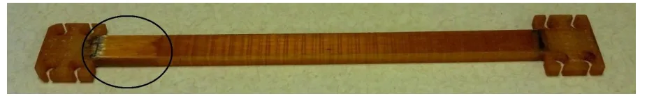
LORD currently produces two different styles of force generators for vibration control, one linear and one circular. This research focuses on the flexure mechanism present on the linear actuators. The current production flexure design performs well, but changes were desired for future production models. These changes, which were implemented prior to the start of this research, primarily reduced the number of parts that make up the flexure mechanism. This reduction in complexity significantly reduces the amount of time required to build an actuator, which directly affects the cost of production. These flexures were made with a composite material for several reasons. Namely, composites are very lightweight as compared to traditional metallic structures, and they can offer very high stiffness values at those low weights. Figure 1.1 below shows one of the composite flexures after endurance testing.
Figure 1.1 Composite Flexure
Unfortunately, these design changes did not lead to a flexure which could be used as a replacement in the production actuators. Upon endurance testing, the flexures failed after a fraction of the time required for the production parts to pass inspection. An area with delamination damage from this testing is circled in Figure 1.1. This research was initiated to investigate the cause of the poor performance as well as to revise the design. Since this flexure could potentially be used as a drop in replacement for the existing production models, there were many restrictions on the geometry of the revised part, but the nature of composite materials allows for many design changes without changing the physical geometry.
1.3OBJECTIVES
The primary goals of this research were to determine the cause of the poor performance of the composite flexures, and to use this knowledge to revise the design. A variety of modeling methods and optimization techniques are used, and the results are verified experimentally. These goals can be broken down further to provide an outline for the project:
Determine the cause of poor performance
o Perform a basic stress analysis using the material properties provided by the composite supplier to ensure the ideal material limits weren’t exceeded during testing
o Verify that the correct procedures were followed by the manufacturer when the parts were made
Revise the design to improve performance
o Determine the best composite material for the flexure application considering fatigue performance, strength and modulus limits, and manufacturing options
o Using the modeling methods discussed in Chapter 2, including Euler-Bernoulli beam theory, classical lamination theory, and free-edge stress models, write an optimization routine which determines the optimal composite stacking sequence
CHAPTER 2
MODELING METHODS
2.1BEAM THEORY
In this section, the flexures are modeled using beam theory and isotropic assumptions. Analytical models are derived using the Euler-Bernoulli beam theory and single degree of freedom vibration theory, and finite element models are created using simple beam elements. These models are used to calculate the deflection, angle of deflection, bending moment, shear force, and natural frequency of the flexures.
2.1.1ANALYTICAL MODELING
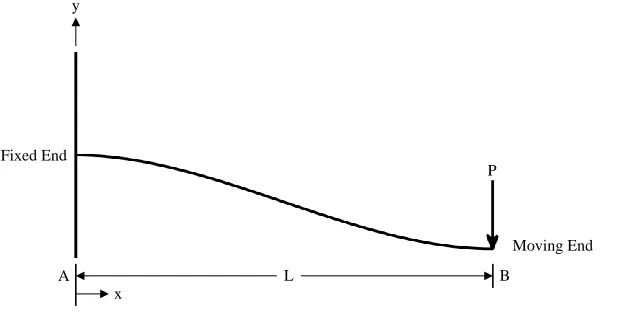
The flexures used on the AVCAs bend with a unique shape, with boundary conditions typically referred to as fixed-guided or fixed-sliding. This implies that both ends always maintains a slope of 0°, shown below in Figure 2.1.
Figure 2.1 Fixed-Guided Deflection Pattern
A L B
P
x y
Fixed End
Starting with a free body diagram and the equation of the elastic curve, the equations for deflection, slope, bending-moment and shear force can be derived for these boundary conditions using the Euler-Bernoulli beam theory. Typical sign conventions are used throughout the derivation. The fixed-guided bending pattern requires three boundary conditions, resulting in three unknown reaction forces and moments to solve for. These reactions are shown in Figure 2.2 along with the applied force, 𝑃.
Figure 2.2 Applied and Reaction Forces on Beam
To solve for the three unknown reactions, three equations will be required. The first of these equations results from summing the forces in the y-direction, and it leads to the value of the reaction force at the fixed end, 𝑅𝐹,𝐴.
The two additional reactions are solved for by integrating the differential equation governing the elastic curve, given below.
P
R
F,AR
M,AR
M,B∑ 𝐹𝑦 = 0 = 𝑅𝐹,𝐴− 𝑃
The internal bending moment, 𝑀(𝑥), can be solved for by looking at a cut section of the beam anywhere in the middle of the span. This location can be labeled as 𝐷, and summing the moments about this point results in the equation which describes the bending moment along the entire length.
Figure 2.3 Cut Beam Section from Fixed End
This equation describes the internal bending moment over the entire length of the beam. Integration can begin after substituting it into the equation of the elastic curve, as well as a substitution for 𝑅𝐹,𝐴.
R
F,AV(x)
M(x)
R
M,AD
x
∑ 𝑀𝐷 = 0 = 𝑅𝐹,𝐴𝑥 + 𝑅𝑀,𝐴− 𝑀(𝑥)
𝑀(𝑥) = 𝑅𝐹,𝐴𝑥 + 𝑅𝑀,𝐴
𝐸𝐼𝑑
2𝑦
𝑑𝑥2 = 𝑀(𝑥) = 𝑅𝐹,𝐴𝑥 + 𝑅𝑀,𝐴 = 𝑃𝑥 + 𝑅𝑀,𝐴
𝐸𝐼𝑑𝑦 𝑑𝑥 =
1 2𝑃𝑥
2 + 𝑅
𝑀,𝐴𝑥 + 𝐶1
𝐸𝐼𝑦 =1 6𝑃𝑥
3+1
2𝑅𝑀,𝐴𝑥
2+ 𝐶
In these equations, 𝐸 represents the elastic modulus and 𝐼 represents the moment of inertia about the neutral axis of the beam, which has a rectangular cross-section. The boundary conditions for this model dictate that the deflection is zero at 𝑥 = 0 and the slope is zero at
𝑥 = 0 and 𝑥 = 𝐿. The two constants of integration along with the unknown reaction moment can be solved for using these conditions. The internal bending moment equation can then be used to solve for the reaction moment at the guided end, 𝑅𝑀,𝐵.
The final resulting equations for deflection, angle of deflection, internal bending moment and internal shear force are given below.
𝑑𝑦
𝑑𝑥|𝑥=0= 0
𝑦𝑖𝑒𝑙𝑑𝑠
→ 𝐶1 = 0
𝑑𝑦 𝑑𝑥|𝑥=𝐿
= 0𝑦𝑖𝑒𝑙𝑑𝑠→ 𝑅𝑀,𝐴= −
𝑃𝐿
2
𝑦|𝑥=0= 0𝑦𝑖𝑒𝑙𝑑𝑠→ 𝐶2 = 0
𝑅𝑀,𝐵 = 𝑀(𝐿) =𝑃𝐿
2
𝑦 = 𝑃𝑥
2
12𝐸𝐼(2𝑥 − 3𝐿) (2.1)
𝜃 = 𝑑𝑦 𝑑𝑥=
𝑃𝑥
2𝐸𝐼(𝑥 − 𝐿) (2.2)
𝑀 = 𝑑
2𝑦
𝑑𝑥2 = 𝑃 (𝑥 −
𝐿
2) (2.3)
𝑉 =𝑑
3𝑦
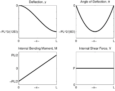
These four equations are plotted across the entire beam length in Figure 2.4. Critical values are also labeled for each curve. Although equations for stress and strain can be derived using this model, they hold no value when the actual composite material is considered. Stress and strain are calculated using classical lamination theory in Section 2.2.
Figure 2.4 Fixed-Guided Beam Bending Results
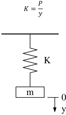
In this equation, 𝐾 represents the bending stiffness and 𝑚 represents the moving mass. The stiffness for a beam in bending can be calculated using
Figure 2.5 Equivalent Single Degree of Freedom Mass and Spring
The deflection, 𝑦, can be calculated at the guided end of the beam (𝑥 = 𝐿) using Equation (2.1) and can be substituted in the above equation to result in
This equation can finally be substituted into Equation (2.5) to calculate the natural frequency of the system,
m
0
y
K
𝜔𝑛 = 2𝜋𝑓𝑛 = √𝐾
𝑚 (2.5)
𝐾 = 𝑃
𝑦 (2.6)
𝐾 =12𝐸𝐼
𝐿3 (2.7)
𝑓𝑛 =
1 2𝜋√
12𝐸𝐼
Although some simplifying assumptions were made in the derivation, this natural frequency calculation is quite accurate. In addition, the above formulas can be manipulated to provide the maximum deflection as a function of frequency,
This equation is particularly useful because the AVCA requirements include force levels across a range of frequencies. If the mass is held constant, as it is in practice, the deflection can be calculated across this range. If the deflection value is ever greater than the allowable limits, an increase in mass or a decrease in force will be necessary.
If a more accurate natural frequency model is desired, the mass of the beam itself can be included in the formulation. The following transcendental equation representing a guided-fixed system can be solved using numerical methods to determine the natural frequency (Özkaya et al., 1997). Note that this formulation reverses the location of the fixed and guided ends as compared to Figure 2.1, so the concentrated end mass is located at 𝑥 = 0.
In this equation, 𝛼 = 𝑚/𝜌𝐴𝐿 represents the ratio between the concentrated mass and the beam mass, and 𝜂 = 𝑥𝑠/𝐿 represents the normalized location of the concentrated mass on the beam (in this case, equal to 0). The constant 𝛽 is referred to as a frequency coefficient, and it can be related to the natural frequency of the system using the following formula (Maurizi & Bellés, 1991).
𝑦 = 𝑃
𝑚(2𝜋𝑓)2 (2.9)
2(cos 𝛽 sinh 𝛽 + sin 𝛽 cosh 𝛽) − 𝛼𝛽{2 cos 𝛽𝜂 cosh 𝛽𝜂 + (cos 𝛽 sinh 𝛽 + sin 𝛽 cosh 𝛽)(sinh 𝛽𝜂 cosh 𝛽𝜂 − cos 𝛽𝜂 sin 𝛽𝜂) + sin 𝛽 sinh 𝛽
∗ (cos2𝛽𝜂 − cosh2𝛽𝜂) − cos 𝛽 cosh 𝛽
∗ (cos2𝛽𝜂 + cosh2𝛽𝜂)} = 0
Although this method is more accurate than others which ignore the beam mass, it requires much more time to solve. An analytical solution, such as Equation (2.8), is more appropriate for an optimization routine.
2.1.2FINITE ELEMENT MODELING
The finite element method can be used to model the flexures at the beam theory level, and this simple implementation can be compared with the analytical models discussed in Section 2.1.1. For the same reasons mentioned previously, only the deflection and natural frequency will be considered as useful output from this model. More advanced finite element models which can accurately model the layered composite stresses are discussed in Section 2.2.2 and Section 2.3.2.
The simple two-node beam element with a total of four degrees of freedom is shown below in Figure 2.6. Each node is allowed to displace vertically in space as well as rotate. This element has C1 continuity, meaning that the deflection and slope must both be
continuous between connected elements. The typical shape functions used to achieve this continuity are the Hermitian cubic shape functions, shown in Figure 2.7. In addition, the effects of transverse shear are neglected in this model, consistent with Euler-Bernoulli beam theory.
𝛽4 =𝜌𝐴𝐿
4𝜔
𝑛2
Figure 2.6 Two-Node Beam Element
Figure 2.7 Hermitian Cubic Shape Functions in Natural Coordinates
The stiffness and consistent mass matrices (𝒌𝒆 and 𝒎𝒆) for this element have been derived in many introductory finite element textbooks (Cook et al., 2002; Chandrupatla & Belegundu, 2012), and are thus listed below without derivation.
q1
q2
q3
q4
1 2
In these equations, 𝐸 is the elastic modulus, 𝐼 is the moment of inertia about the neutral axis,
𝑙𝑒 is the length of the element, 𝐴𝑒 is the cross sectional area of the element, and 𝜌 is the
material volumetric density.
The global stiffness and mass matrices (𝑲 and 𝑴) are assembled for the entire model, along with the global force matrix, 𝑭, and boundary conditions are easily applied by suppressing the appropriate degrees of freedom. The solution of Equation (2.14) presents the deflection and slope results at every node, 𝑸, while solving Equation (2.15) allows for the calculation of the natural frequencies, 𝜆, where 𝜆 = 𝜔𝑛2, and mode shapes, 𝑼. These are the
eigenvalues and eigenvectors, respectively. Although frequencies above the fundamental are not relevant to this research, this method also allows for their calculation.
This method can easily be implemented using a computational program such as MATLAB, though it can also be coded in a variety of other computer languages. Advanced finite element packages are not required for this level of analysis.
𝒌𝒆 =𝐸𝐼 𝑙𝑒3
[
12 6𝑙𝑒 −12 6𝑙𝑒
6𝑙𝑒 4𝑙𝑒2 −6𝑙
𝑒 2𝑙𝑒2
−12 −6𝑙𝑒 12 −6𝑙𝑒
6𝑙𝑒 2𝑙𝑒2 −6𝑙𝑒 4𝑙𝑒2 ]
(2.12)
𝒎𝒆=𝜌𝐴𝑒𝑙𝑒
420 [
156 22𝑙𝑒 54 −13𝑙𝑒
22𝑙𝑒 4𝑙𝑒2 13𝑙𝑒 −3𝑙𝑒2
54 13𝑙𝑒 156 −22𝑙𝑒
−13𝑙𝑒 −3𝑙𝑒2 −22𝑙𝑒 4𝑙𝑒2 ]
(2.13)
𝑲𝑸 = 𝑭 (2.14)
2.2CLASSICAL LAMINATION THEORY
The flexures are made out of a layered, orthotropic composite material, so the beam theory models are not able to accurately predict the state of stress in the laminate. To do this, classical lamination theory is used, which is similar to classical plate theory. However, whereas plate theory typically assumes isotropic material properties, lamination theory allows for orthotropic material properties applied to each individual layer, or lamina.
2.2.1ANALYTICAL MODELING
The classical lamination theory forms a set of closed form relations, and thus is considered an analytical technique. There are several assumptions present in the derivation of the theory, and these are listed in texts on the subject (Daniel & Ishai, 2006). One such assumption, as with classical beam theory, is that the effects of transverse shear are negligible. This is justified by assuming that the laminate is thin. Another assumption is that the layers are perfectly bonded together, meaning there is no slippage between layers and the infinitesimal bond does not fail.
There are many texts which cover classical lamination theory derivations, so the details will not be included here. Only the overall ideas will be presented, the first of which are the kinematic strain-displacement equations given below.
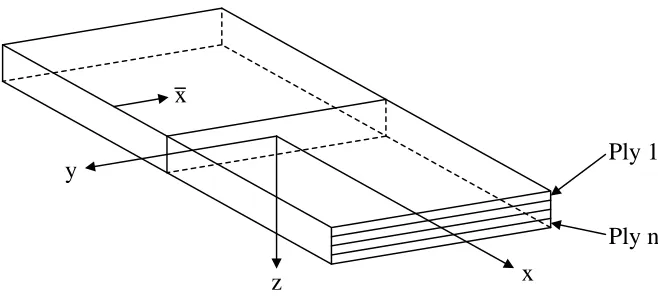
Figure 2.8 (a) Laminate Section (b) Positive Angle Definition (Daniel & Ishai, 2006)
The 𝑢0, 𝑣0, and 𝑤 variables correspond to the displacements of the reference (or middle) plane in the x, y, and z directions. These equations allow for the calculation of strain at any point in the laminate from the reference plane strains and curvatures.
The stress-strain relations for an individual layer 𝑘 are given below, first with respect to its own material axes (1-2), and secondly with respect to the laminate coordinate system
z y x x y 1 2 θ (a) (b) [ 𝜀𝑥 𝜀𝑦 𝛾𝑠] = [
𝜀𝑥0
𝜀𝑦0 𝛾𝑠0
] + 𝑧 [ 𝜅𝑥 𝜅𝑦 𝜅𝑠] = [ 𝜕𝑢0 𝜕𝑥 𝜕𝑣0 𝜕𝑦 𝜕𝑢0 𝜕𝑦 + 𝜕𝑣0 𝜕𝑥 ] − 𝑧 [ 𝜕2𝑤
𝜕𝑥2
𝜕2𝑤
𝜕𝑦2
2 𝜕
2𝑤
𝜕𝑥𝜕𝑦]
The reduced stiffness matrix for an orthotropic layer, [𝑄]𝑘, and the transformation matrix,
[𝑇], are given below.
After some substitution, an expression relating the stresses to the reference plane strains and curvatures can be obtained.
Comparing Equations (2.16) and (2.21), it can be seen that the strains vary linearly through the entire laminate while the stresses only vary linearly through each layer. Discontinuities can occur in the stresses between layers when they are oriented at different angles.
Due to the stress discontinuities between layers, it is more straightforward to integrate and sum the stresses over each layer than work with the laminate as a whole. To do this, expressions relating the force and moments to deformation need to be defined. Resultant
[ 𝜎1
𝜎2 𝜏6]𝑘= [
𝑄11 𝑄12 0
𝑄21 𝑄22 0
0 0 𝑄66
]
𝑘
[ 𝜀1
𝜀2
𝛾6]𝑘= [𝑄] [ 𝜀1
𝜀2
𝛾6]𝑘 (2.17)
[ 𝜎𝑥 𝜎𝑦 𝜏𝑠]𝑘 = [ 𝑄𝑥𝑥 𝑄𝑥𝑦 𝑄𝑥𝑠 𝑄𝑦𝑥 𝑄𝑦𝑦 𝑄𝑦𝑠 𝑄𝑠𝑥 𝑄𝑠𝑦 𝑄𝑠𝑠 ] 𝑘 [ 𝜀𝑥 𝜀𝑦 𝛾𝑠]𝑘 = [𝑇] −1[𝑄] 𝑘[𝑇]−𝑇[ 𝜀𝑥 𝜀𝑦 𝛾𝑠]𝑘 = [𝑄̅]𝑘[ 𝜀𝑥 𝜀𝑦
𝛾𝑠]𝑘 (2.18)
[𝑄]𝑘 = [
𝑄11 𝑄12 0
𝑄21 𝑄22 0
0 0 𝑄66
]
𝑘
=
[ 𝐸1 1 − 𝜈12𝜈21
𝜈21𝐸1 1 − 𝜈12𝜈21
0
𝜈12𝐸2 1 − 𝜈12𝜈21
𝐸2 1 − 𝜈12𝜈21
0
0 0 𝐺12]𝑘
(2.19)
[𝑇] = [ cos
2𝜃 sin2𝜃 2 sin 𝜃 cos 𝜃
sin2𝜃 cos2𝜃 −2 sin 𝜃 cos 𝜃
− sin θ cos θ sin 𝜃 cos 𝜃 cos2𝜃 − sin2𝜃
] (2.20)
[ 𝜎𝑥
𝜎𝑦
𝜏𝑠]𝑘 = [𝑄̅]𝑘[ 𝜀𝑥0
𝜀𝑦0 𝛾𝑠0
] + 𝑧[𝑄̅]𝑘[
𝜅𝑥
𝜅𝑦
forces and moments can substituted for the stresses acting on a layer 𝑘, shown below in Figure 2.9. The force resultants 𝑁𝑥, 𝑁𝑦, and 𝑁𝑠 have units of force per unit length while the moment resultants 𝑀𝑥, 𝑀𝑦, and 𝑀𝑠 have units of moment per unit length, or simply force.
Figure 2.9 (a) Force Resultants (b) Moment Resultants (Nettles, 1994)
For an 𝑛-ply laminate, the total force and moment resultants are obtained by summing the stresses over each individual layer.
With the z-axis taken as positive upwards, layer number 1 (𝑘 = 1) will be the bottom layer of the laminate. The variables 𝑧𝑘 and 𝑧𝑘−1 correspond to the upper and lower 𝑧
-coordinates of layer 𝑘, referenced from the midplane of the laminate. Values of 𝑧 below the
z
(a) x
y
The stress equations obtained in Equation (2.21) can be substituted into Equations (2.22) and (2.23), leading to the laminate stiffness matrices [𝐴], [𝐵], and [𝐷] after simplification.
These equations can be combined to produce a single expression that relates the force and moments to the reference plane strains and curvatures.
This is often reduced to
In the flexure application, the loads are known ahead of time, rather than the strains and curvatures, so the relationship in Equation (2.28) needs to be rewritten using the inverse of the [𝐴𝐵𝐷] matrix, referred to as the [𝑎𝑏𝑐𝑑] matrix.
𝐴𝑖𝑗= ∑[𝑄̅𝑖𝑗]𝑘 𝑛
𝑘=1
(𝑧𝑘− 𝑧𝑘−1) (2.24)
𝐵𝑖𝑗 =
1
2∑[𝑄̅𝑖𝑗]𝑘 𝑛
𝑘=1
(𝑧𝑘2− 𝑧
𝑘−12 ) (2.25)
𝐷𝑖𝑗= 1
3∑[𝑄̅𝑖𝑗]𝑘 𝑛
𝑘=1
(𝑧𝑘3− 𝑧
𝑘−13 ) (2.26)
[ 𝑁𝑥 𝑁𝑦 𝑁𝑠 𝑀𝑥 𝑀𝑦 𝑀𝑠] = [ 𝐴𝑥𝑥 𝐴𝑥𝑦 𝐴𝑥𝑠 𝐵𝑥𝑥 𝐵𝑥𝑦 𝐵𝑥𝑠 𝐴𝑦𝑥 𝐴𝑦𝑦 𝐴𝑦𝑠 𝐵𝑦𝑥 𝐵𝑦𝑦 𝐵𝑦𝑠 𝐴𝑠𝑥 𝐴𝑠𝑦 𝐴𝑠𝑠 𝐵𝑠𝑥 𝐵𝑠𝑦 𝐵𝑠𝑠 𝐵𝑥𝑥 𝐵𝑥𝑦 𝐵𝑥𝑠 𝐷𝑥𝑥 𝐷𝑥𝑦 𝐷𝑥𝑠 𝐵𝑦𝑥 𝐵𝑦𝑦 𝐵𝑦𝑠 𝐷𝑦𝑥 𝐷𝑦𝑦 𝐷𝑦𝑠 𝐵𝑠𝑥 𝐵𝑠𝑦 𝐵𝑠𝑠 𝐷𝑠𝑥 𝐷𝑠𝑦 𝐷𝑠𝑠][
𝜀𝑥0
𝜀𝑦0
𝛾𝑠0
𝜅𝑥 𝜅𝑦 𝜅𝑠] (2.27) [𝑁 𝑀] = [ 𝐴 𝐵 𝐵 𝐷] [𝜀 0
𝜅] (2.28)
[𝜀0 𝜅] = [ 𝐴 𝐵 𝐵 𝐷] −1 [𝑁 𝑀] = [ 𝑎 𝑏 𝑐 𝑑] [ 𝑁
Using these equations, the stresses and strains in each layer of a laminated structure can be determined from the applied force and moments.
Another key aspect of this model is the ability to predict the material properties of the laminate as a whole, since layers at varying angles will contribute different amounts of stiffness to the laminate. The only property required for the flexure application is the laminate bending modulus, typically referred to as 𝐸𝑥𝑏. This is unique from the elastic
modulus along the laminate x or y axes, and it can be computed from Equation (2.31), where
ℎ is the total laminate thickness (Barbero, 2011).
An important aspect of any laminated material is the stacking sequence. Depending on the orientation and order in which the layers are placed, couplings between different modes of deformation may be introduced, which are undesirable in this research. Examples of these couplings include extension/bending coupling, shear coupling, and torsion coupling. In order to suppress these effects, a symmetric and balanced laminate can be designed. The symmetry refers to symmetry about the midplane (or reference plane) of that laminate, while the balancing implies that for every positive angle ply, there is also a ply at the same negative
[𝑎 𝑏 𝑐 𝑑] = [ 𝑎𝑥𝑥 𝑎𝑥𝑦 𝑎𝑥𝑠 𝑏𝑥𝑥 𝑏𝑥𝑦 𝑏𝑥𝑠 𝑎𝑦𝑥 𝑎𝑦𝑦 𝑎𝑦𝑠 𝑏𝑦𝑥 𝑏𝑦𝑦 𝑏𝑦𝑠 𝑎𝑠𝑥 𝑎𝑠𝑦 𝑎𝑠𝑠 𝑏𝑠𝑥 𝑏𝑠𝑦 𝑏𝑠𝑠 𝑐𝑥𝑥 𝑐𝑥𝑦 𝑐𝑥𝑠 𝑑𝑥𝑥 𝑑𝑥𝑦 𝑑𝑥𝑠 𝑐𝑦𝑥 𝑐𝑦𝑦 𝑐𝑦𝑠 𝑑𝑦𝑥 𝑑𝑦𝑦 𝑑𝑦𝑠 𝑐𝑠𝑥 𝑐𝑠𝑦 𝑐𝑠𝑠 𝑑𝑠𝑥 𝑑𝑠𝑦 𝑑𝑠𝑠] (2.30)
𝐸𝑥𝑏 = 12 ℎ3𝑑
𝑥𝑥
= 12(𝐷𝑥𝑥𝐷𝑦𝑦− 𝐷𝑥𝑦
2 )
ℎ3𝐷 𝑦𝑦
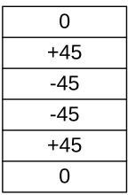
angle somewhere in the laminate. An example of a symmetric and balanced laminate is given below in Figure 2.10.
Figure 2.10 Symmetric Balanced Laminate Example
In standard laminate notation, this example layup can be described as [0°,±45°]s (Daniel &
Ishai, 2006). Only symmetric and balanced layups will be considered for the flexure design.
2.2.2FINITE ELEMENT MODELING
This level of finite element analysis can still be implemented in code by an experienced user, but it is more complex as compared to the beam theory model discussed in Section 2.1.2. Rather than doing this, the commercial package ANSYS was used to do all the laminated composite modeling. There are many element and modeling choices available in ANSYS for this level of analysis, and the decision on which to use should be made on the details available in the reference documentation as well as literature on the subject.
The two types of elements typically used in modeling composite materials are plates and shells, though in practice, shells are used more since they can effectively become a plate by applying no initial curvature (Barbero, 2014; Cook et al., 2002). These elements can employ various plate theories in their construction, two of which are the Kirchhoff theory
0 +45
-45 -45 +45
and the Mindlin-Reissner theory. The Kirchhoff theory assumptions correspond to the assumptions made in the Bernoulli-Euler beam finite elements, especially in regards to the transverse shear being considered negligible. Just as the 1D beams required C1 continuity between elements, the 2D Kirchhoff theory plates also share this requirement. Unfortunately, this is much more difficult to implement in 2D than 1D, and most elements in this category require ad hoc methods to be useable (Cook et al., 2002).
The Mindlin-Reissner theory corresponds with the Timoshenko beam theory, where transverse shear is accounted for in the formulation. This method requires more degrees of freedom as compared to the Kirchhoff theory, but it only requires C0 continuity in its implementation. Elements which fulfill this requirement are readily available, though they aren’t without problems. Issues such as shear locking when elements are thin and spurious modes due to underintegration can appear, though much research has been put towards developing elements which avoid these shortcomings.
In ANSYS, the two elements used in this research are the SHELL181 and SHELL281. These shell models are both governed by the Mindlin-Reissner theory, and they are both well-suited for modeling thin to moderately-thick composites. The default element behavior of these two shells automatically handles many of the shear locking and spurious energy mode problems.
solve. The best choice of element is not typically obvious, but test cases can be used to determine if a significant performance difference exists. Depending on the size of the model and the available computing power, the difference may be negligible. Both elements are shown in Figure 2.11(a) and (b) with their nodal locations and positive coordinate axes labeled.
Figure 2.11 (a) SHELL181 Element (b) SHELL281 Element (ANSYS Inc., 2013)
Both the SHELL181 and SHELL281 elements support a layered input, meaning that each element can be made up of several layers of material. This means that composite laminates do not need to use one element per layer, but many layers can be modeled by a single element. The elements place integration points through the thickness to calculate the individual ply outputs, including the stresses and strains.
2.3FREE EDGE STRESSES
The stresses calculated using classical lamination theory are accurate for thin laminates, but they are only applicable for the interior of the material away from the free edges. Near these edges, depicted in Figure 2.12, the stress state becomes three dimensional in nature (Pipes & Pagano, 1970).
Figure 2.12 Laminate Free Edge Stress Regions
For a laminate subjected to an out-of-plane shear and bending load, only the in-plane stresses 𝜎𝑥, 𝜎𝑦, and 𝜏𝑥𝑦 exist in the interior, along with the single interlaminar stress 𝜏𝑥𝑧.
This is the type of loading experienced by the fixed-guided flexures. Classical lamination theory does not directly predict the interlaminar stress 𝜏𝑥𝑧 in the laminate interior, though it
can be calculated using other methods if desired. The remaining two interlaminar stresses, 𝜎𝑧
and 𝜏𝑦𝑧, only exist near the free edge. The introduction of these two stresses leads to variations in the four interior stresses as the free edge is approached. These variations are dictated by the equations of stress equilibrium, which are listed below in Cartesian coordinates without body forces.
x
y z
Free edge Free edge
𝜕𝜎𝑥 𝜕𝑥 +
𝜕𝜏𝑦𝑥
𝜕𝑦 +
𝜕𝜏𝑧𝑥 𝜕𝑧 = 0
𝜕𝜏𝑥𝑦
𝜕𝑥 +
𝜕𝜎𝑦
𝜕𝑦 + 𝜕𝜏𝑧𝑦
This level of stress analysis is not always necessary when evaluating a laminate, however, as composites continue to make the transition from secondary to primary structural components, it becomes more important to reduce the potential for delamination resulting from high interlaminar stresses near free edges (Reddy, 2004). The in-plane stresses are not typically considered as contributors to delamination, so even though their variations at the free edge can be calculated, only the interlaminar stresses are necessary. By excluding the in-plane stress calculation at the free edge, valuable computation time can be saved when analyzing a large number of layups.
These free edge effects were first researched by Pipes & Pagano (1970), and many papers have been published on the subject since that time. These papers can generally be divided into analytical methods and finite element methods. Though finite element methods are powerful and useful over a large variety of geometries, analytical methods are much faster where applicable. The flexures have simple rectangular cross sections, so the analytical methods can be used for both general design and optimization. However, the vast majority of analytical free edge papers only consider a laminate under longitudinal loading. There are several papers which consider a laminate in pure bending, but only two papers were found which consider the effects of out-of-plane shear in addition to bending (Kassapoglou, 1990; Kim & Atluri, 1994).
2.3.1ANALYTICAL MODELING
symmetric. This method allows for axial loads, bending moments and out-of-plane shear loads to be applied to the laminate. Although the flexures do not experience an axial load, they do experience a bending moment and shear force as calculated using beam theory. These loads vary along the flexure length, so only the cross-section with the largest values needs to be considered for the free edge analysis. An examination of Equations (2.3) and (2.4) reveals that the shear load is constant everywhere, but the maximum bending moment occurs at either the fixed or guided end. For the purposes of this analysis, only the guided end will be considered. It is worth noting that this method originally only considered a cantilever beam, but there were no restrictions in the derivation limiting the analysis to these boundary conditions. Rather, the author simply assumed a moment distribution of 𝑀 = 𝑉𝑑, where 𝑑 is the distance from the fixed end to the point of shear load, 𝑉. This assumption is easily overcome by using the moment distribution determined from beam theory for the fixed-guided boundary conditions.
Before going into the details of this method, we point out that when discussing the stresses in ply 𝑘, ply number 1 is considered to be the top layer of the laminate. This is the opposite of the established ply number scheme, so the ply numbering must be reversed after calculating the results from classical lamination theory. Finally, an additional coordinate variable 𝑥̅ is introduced which originates at the free edge and points towards the laminate interior, illustrated in Figure 2.13.
far-Figure 2.13 Free Edge Stress Coordinate System
This method uses classical lamination theory to predict the far-field stress state which leads to a linear stress distribution through the thickness each layer. Six constants are defined using these stress results, given below.
The 𝑧 variable is used to describe the vertical location within each layer. It is equal to zero at the bottom of each layer 𝑘, and equal to the layer thickness 𝑡𝑘 at the top of each respective
layer. Together, these equations describe the far-field behavior of the in-plane stresses. Though the 𝑧 dependence of the in-plane stresses is assumed, no such assumption is made regarding the variation in the 𝑥̅ direction. This unknown variation is introduced through the variables 𝑔1 and 𝑔2, along with their derivatives with respect to 𝑥̅: 𝑔1′, 𝑔1′′, and 𝑔2′. These variables are present in the three interlaminar stress equations for each ply, given below.
x y
z x
Ply 1
Ply n
𝜎𝑦𝑘 = 𝐴0𝑘+ 𝐴1𝑘𝑧 (2.33)
𝜎𝑥𝑦𝑘 = 𝐵0𝑘+ 𝐵1𝑘𝑧 (2.34)
The constants 𝐶0𝑘, 𝐶
1𝑘, and 𝐷0𝑘 force interlaminar stress continuity at all ply interfaces, and
can be determined using the previously defined constants 𝐴0𝑘, 𝐴1𝑘, 𝐵0𝑘, and 𝐵1𝑘.
The variable 𝑡𝑏𝑘 is the distance from the laminate midplane (in 𝑧) to the bottom of layer 𝑘, and ℎ is the total laminate thickness.
In order to solve the interlaminar stress equations, the unknown functions 𝑔1 and 𝑔2
must be determined. To do this, the complimentary energy, 𝛱𝑐, is minimized for the laminate using calculus of variations resulting in two coupled differential equations. For clarity, the laminate complementary energy equation and the resulting differential equations are given below.
𝜎𝑧𝑘 =
1
ℎ2𝑔1′′(𝐶1𝑘+ 𝐶0𝑘𝑧 + 𝐴0𝑘
𝑧2 2 + 𝐴1
𝑘𝑧
3
6) (2.36)
𝜏𝑦𝑧𝑘 =1
ℎ𝑔1
′(𝐶
0𝑘+ 𝐴0𝑘𝑧 + 𝐴1𝑘
𝑧2
2) (2.37)
𝜏𝑥𝑧𝑘 =1
ℎ𝑔2
′ (𝐷
0𝑘+ 𝐵0𝑘𝑧 + 𝐵1𝑘
𝑧2 2) +
6𝑉 ℎ (
1 4−
(𝑡𝑏𝑘+ 𝑧)2
ℎ2 ) (2.38)
𝐶0𝑘= − ∑ (𝐴0𝑖𝑡𝑖+ 𝐴1𝑖 (𝑡
𝑖)2
2 )
𝑘
𝑖=1
(2.39)
𝐶1𝑘 = − ∑ (𝐴0𝑖
(𝑡𝑖)2
2 + 𝐴1
𝑖 (𝑡
𝑖)3
6 + 𝐶0
𝑖𝑡𝑖)
𝑘
𝑖=1
(2.40)
𝐷0𝑘= − ∑ (𝐵0𝑖𝑡𝑖+ 𝐵1𝑖
(𝑡𝑖)2
2 )
𝑘
𝑖=1
After substituting the stress equations in terms of 𝑔1 and 𝑔2 and differentiating, two ordinary differential equations are obtained, given below. It should be noted that the stress vector 𝜎 in Equation (2.42) includes all six stress components, not just the three interlaminar stresses, and the 𝑆 matrix is the full six by six compliance matrix for each ply. The additional stress equations are provided by Kassapoglou (1990).
The various 𝑅 coefficients represent ratios between integrals, provided in Kassapoglou (1990). After assuming a solution of the form 𝑎𝑒𝑚𝑥̅ for 𝑔
1 and 𝑔2, the characteristic equation
below is found for 𝑚.
After considering the six possible solutions to this equation, only the three with negative real parts are accepted, as positive real parts would cause the interlaminar stresses to grow towards the interior of the laminate, rather than diminish. This leads to the following equations for 𝑔1 and 𝑔2.
𝑑2 𝑑𝑥̅2(
𝜕𝛱𝑐
𝜕𝑔1′′) −
𝑑 𝑑𝑥̅(
𝜕𝛱𝑐
𝜕𝑔1′) +
𝜕𝛱𝑐
𝜕𝑔1 = 0 (2.43)
𝑑 𝑑𝑥̅(
𝜕𝛱𝑐 𝜕𝑔2′) −
𝜕𝛱𝑐 𝜕𝑔2
= 0 (2.44)
𝑑4𝑔1 𝑑𝑥̅4 + 𝑅1
𝑑2𝑔1
𝑑𝑥̅2 + 𝑅2𝑔1+ 𝑅3
𝑑2𝑔2
𝑑𝑥̅2 + 𝑅4𝑔2 = 0 (2.45)
𝑑2𝑔2
𝑑𝑥̅2 + 𝑅5𝑔2+ 𝑅6
𝑑2𝑔1
𝑑𝑥̅2 + 𝑅7𝑔1 = 0 (2.46)
𝑚6+ (𝑅1+ 𝑅5 − 𝑅3𝑅6)𝑚4+ (𝑅
1𝑅5 + 𝑅2− 𝑅3𝑅7
− 𝑅4𝑅6)𝑚2+ 𝑅
2𝑅5 − 𝑅4𝑅7 = 0
(2.47)
To solve for 𝑆𝑖 and 𝑆̅𝑖, the three boundary conditions and one final equation must be
used.
With 𝑔1 and 𝑔2 fully determined, the free edge stress distribution can be calculated and compared for various ply layups.
2.3.2FINITE ELEMENT MODELING
The free edge stress effect is three dimensional in nature, and as such cannot be accurately modeled using plate or shell finite elements. Solid elements are necessary for this level of analysis, and ANSYS provides options which allow for laminations to model composite materials. Two of the most useful elements for this purpose are labeled as SOLID185 and SOLID186 (Barbero, 2014).
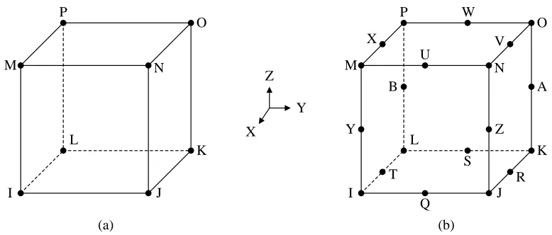
SOLID185 is a solid hexahedra which exhibits quadratic displacement behavior in three dimensional space (ANSYS Inc., 2013). It has eight nodes, each with three displacement degrees of freedom, 𝑢𝑥, 𝑢𝑦, and 𝑢𝑧. SOLID186 is similar, but with twenty total nodes to more accurately model complex structures. These elements are shown in Figure
𝑔2 = 𝑆̅1𝑒𝑚1𝑥̅+ 𝑆̅
2𝑒𝑚2𝑥̅+ 𝑆̅3𝑒𝑚3𝑥̅ (2.49)
𝑆1+ 𝑆2 + 𝑆3 = −1 (2.50)
𝑆̅1+ 𝑆̅2 + 𝑆̅3 = −1 (2.51)
𝑆1𝑚1+ 𝑆2𝑚2 + 𝑆3𝑚3 = 0 (2.52)
𝑆𝑖
𝑆̅𝑖
= − 𝑚𝑖
2+ 𝑅
5
𝑅6𝑚𝑖2+ 𝑅 7
plate and shell elements described in Section 2.2.2, rotational degrees of freedom are not present in these solid elements.
Figure 2.14 (a) SOLID185 Element (b) SOLID186 Element (ANSYS Inc., 2013)
It is common to increase the mesh density wherever high stress gradients are expected in finite element models, resulting in a smaller element size as the free edge is approached. However, as more elements are included in the analysis, the computation time will increase rapidly. Some level of trial and error must be used to determine the level of mesh density which provides an adequate stress resolution and best utilizes the available computing power. An example of an increased mesh density near a free edge is shown in Figure 2.15.
(b) I J K L M N O P (a) I J K L M N O P Y Z
X Y Z
It is important to note that weak stress singularities exist at the free edge for both 𝜎𝑧
and 𝜏𝑥𝑧 due to homogenous layer assumptions (Wang & Choi, 1982). Finite element analysis does not handle these singularities well, and the stress value at the free edge will be highly influenced by the mesh density. While increasing the density will more accurately predict the stresses prior to reaching the free edge, it will also lead to a meaningless increase in the stress amplitude at the edge itself. For this reason, further considerations must be made prior to using free edge stress values in a failure criterion. These considerations are discussed in Section 2.4.2.
2.4FAILURE CRITERIA
2.4.1INTERIOR STRESSES
One of the most commonly used failure theories for composite laminates is the Tsai-Wu theory, also known as the interactive tensor polynomial theory (Tsai & Tsai-Wu, 1971; Daniel & Ishai, 2006). It is considered an interactive theory, where all the stress components are present in a single expression for predicting failure. In general, it is applicable for a full three-dimensional stress state, but it can be simplified for two-dimensional situations as well. For a state of plane stress, the criterion in given below.
Classical lamination theory predicts a plane stress state for the laminate interior, so the resulting stresses can be substituted into the above equation to determine whether first ply failure has occurred. It is important to note that the subscripts in Equation (2.54) indicate that the stresses should be evaluated in the lamina coordinate system (1-2), not the laminate coordinate system (x-y). The 𝑓 coefficients are defined below.
𝑓1𝜎1+ 𝑓2𝜎2+ 𝑓11𝜎12+ 𝑓22𝜎22+ 𝑓66𝜏62+ 2𝑓12𝜎1𝜎2 = 1 (2.54)
𝑓1 = 1 𝐹1𝑡−
1
𝐹1𝑐 (2.55)
𝑓11= 1
𝐹1𝑡𝐹1𝑐 (2.56)
𝑓2 = 1 𝐹2𝑡−
1
𝐹2𝑐 (2.57)
𝑓22= 1
𝐹2𝑡𝐹2𝑐 (2.58)
𝑓66= 1
𝐹62 (2.59)
In these equations, the 𝐹 terms represent the lamina strength values. 𝐹1𝑡 and 𝐹1𝑐 are the
longitudinal strengths in tension and compression, 𝐹2𝑡 and 𝐹2𝑐 are the transverse strengths in tension and compression, and 𝐹6 is the in-plane shear strength.
It is possible to calculate a factor of safety for the interior using this failure theory by multiplying each stress term in Equation (2.54) by 𝑆𝑓 and solving the resulting quadratic
equation, given below.
When analyzing a laminate, this criterion is applied to each layer individually. The smallest safety factor after considering every layer is taken as the overall safety factor for the laminate interior.
2.4.2FREE EDGE STRESSES
When the potential for failure at the free edge is considered, the primary failure mechanism is typically delamination due to the interlaminar stresses. One failure criterion created for analyzing this situation is referred to as the Quadratic Delamination Criterion, given below (Brewer & Lagace, 1988).
𝑎𝑆𝑓2+ 𝑏𝑆𝑓− 1 = 0 (2.61)
𝑎 = 𝑓11𝜎12+ 𝑓22𝜎22+ 𝑓66𝜏62+ 2𝑓12𝜎1𝜎2 (2.62)
𝑏 = 𝑓1𝜎1+ 𝑓2𝜎2 (2.63)
𝑆𝑓 =−𝑏 + √𝑏
2+ 4𝑎
2𝑎 (2.64)
This criterion uses the concept of an average stresses near the free edge, as it has been shown that weak singularities exist in both 𝜎𝑧 and 𝜏𝑥𝑧 as the free edge is approached (Wang & Choi, 1982). To avoid sensitivity to the artificial stress values predicted right at the free edge, an average stress value is defined below.
The idea behind this averaging is illustrated in Figure 2.16 using an arbitrary interlaminar shear stress distribution. The variable 𝑏 represents the half-width of the laminate, and 𝑥𝑎𝑣𝑔 is the distance over which the averaging is performed. This value is usually determined by fitting experimental data, but it is on the order of one ply thickness. For this research, setting the averaging distance to the ply thickness is sufficient.
Figure 2.16 Average Stress Definition (Gibson, 2007)
y
b
xavg
τxz
Interlaminar shear stress, τxz
After performing an order of magnitude analysis and comparing experimental results, it was determined that a simplified version of the criterion is sufficient for modeling failure at the free edge, given below (Brewer & Lagace, 1988).
This simplification arose from the fact that the compressive interlaminar normal stress 𝜎̅𝑧𝑐
and the interlaminar shear stress 𝜏̅𝑦𝑧 did not significantly affect the results.
The free edge factor of safety calculation proceeds in the same manner as used for the interior stresses. The resulting equations are given below.
The smallest safety factor after considering every layer is taken as the overall safety factor for the laminate free edge.
(𝜏̅𝑥𝑧 𝐹5 ) 2 + (𝜎̅𝑧 𝑡 𝐹3𝑡 ) 2
= 1 (2.67)
𝑎𝑆𝑓2− 1 = 0 (2.68)
𝑎 = (𝜏̅𝑥𝑧 𝐹5 ) 2 + (𝜎̅𝑧 𝑡 𝐹3𝑡 ) 2 (2.69)
𝑆𝑓 = √4𝑎
2𝑎 =
1
CHAPTER 3
INITIAL DESIGN
Prior to the start of this research, a prototype composite flexure, referred to as the initial design, was created to investigate the possibility of replacing the current production flexures. This initial design was subjected to endurance testing which revealed poor fatigue performance, so it was necessary to determine the potential causes of the issue. The first goals of this research were to perform additional experimental testing on these flexures, and to analyze the resulting data in order to make improvements for future designs.
3.1DESIGN DESCRIPTION
Much of the initial design work was focused on the geometry of the flexure to ensure if could be retrofitted on the production actuators. The actual composite layup was considered, but no layup optimization was performed, and the natural frequency was not expected to match any of the production actuators. A CAD model of the design is shown in Figure 3.1, and the manufactured flexure can be seen in Figure 1.1.
Figure 3.1 Initial Design CAD Model
Figure 3.2 Initial Design Ply Layout
This particular design was created using an injection molding process. The sheets of fiber were placed into the mold dry, where each sheet would form a single ply layer. After the layup was complete, the mold was closed and the epoxy resin was injected to fill all the
x
z
3.2EXPERIMENTAL WORK
Some early endurance testing on this initial design suggested poor performance, as the natural frequency decayed appreciably after less than 100 hours of testing. Though further endurance testing was required, it was important to first measure the composite material properties and determine if they matched the expected values from the supplier.
3.2.1MATERIAL PROPERTY TESTING
To test the material properties of the flexures, samples of the material which had not been subject to wear were required. Scraps from the water jet process were used for this purpose, and for this testing, the effect of the ±45° center ply was neglected. The geometry and nominal dimensions of one of these sample specimens is given below. For accuracy, each specimen was measured using calipers prior to testing.
Figure 3.3 Sample Specimen Geometry and Nominal Dimensions
The available testing facility was restricted to measuring the longitudinal and bending (or flexural) modulus of the composite material. However, the available material left over from the water jet process was on the order of 5 mm thick, and the ASTM recommended specimen thickness for tensile testing is 1 mm (ASTM, 2008). Tensile testing with the
Span Length, L [77 mm] Total Length [~150 mm]
Height, h [~4.9 mm]
available specimens was still attempted to determine the longitudinal modulus, but was inconclusive due to inadequate clamping conditions, resulting in the specimens experiencing both slippage and failure under the clamps. Therefore, the data was not analyzed.
Figure 3.4 Three-point Bending Test
The formula for determining the bending modulus from experimental load data is given below.
The variables 𝑤 and ℎ are the width and height of the specimen, 𝐿 is the distance between the outer two roller supports (labeled as Span Length in Figure 3.3), and 𝑠 represents the slope of the linear portion of the load-deflection curve. The results of the three-point testing, provided in Table 3.1, show that the bending modulus of this composite material was approximately 27 GPa for both test dates. Though bending modulus data was not available from the material supplier, classical lamination theory predicts that the bending modulus of a specimen with only 0° layers will be equal to its longitudinal modulus. If the center ±45° ply of the flexure is ignored, this relationship should hold true. However, for this material, the longitudinal
𝐸𝑥𝑏 = 𝐿
3𝑠
modulus provided by the supplier ranges from 53 to 59 GPa, depending on the fiber volume percentage. The discrepancy between these values and the measured bending modulus is considerable, though it is not yet known if this is due only to the under prediction of the three-point bending test, or if a problem also exists in the manufacturing process.
Table 3.1 Bending Modulus Results Test
Date
Sample #1
𝑬𝒙𝒃 [GPa]
Sample #2
𝑬𝒙𝒃 [GPa]
Sample #3
𝑬𝒙𝒃 [GPa]
Sample #4
𝑬𝒙𝒃 [GPa]
Sample #5
𝑬𝒙𝒃 [GPa]
Avg. 𝑬𝒙𝒃 [GPa]
Standard Deviation [MPa]
5/24/2013 27.09 27.28 27.30 26.63 26.36 26.93 420.78
8/13/2013 26.94 27.56 27.72 27.86 27.50 27.52 352.68
If the bending modulus measures around half the expected value, it can reasonably be assumed that other material properties, including the strength values, are lower than the data provided by the supplier as well. However, without the resources to measure any of these properties, no definitive conclusions can be drawn regarding the extent of the performance decrease.
3.2.2ENDURANCE TESTING
The primary measure of actuator performance decay is the natural frequency drop over time. As the flexures experience wear, they lose stiffness and thus the natural frequency decays. If the stress on the flexures is too high, fibers will begin to break and the natural frequency drop will be substantial. In practice this is unacceptable, as the actuators are typically installed in locations on a helicopter where maintenance is not possible. The flexures must remain near their initial natural frequency for the entire life of the helicopter, taken as about 20,000 hours of actuator run time. Depending on the operational frequency of the actuator, this can be on the order of 109 cycles. For this reason, flexure fatigue performance is critical.
Figure 3.5 Initial Design Endurance Test Results
As expected, the results from this endurance test are very poor. The natural frequency dropped almost 2 Hz (9%) during the test which ran for about 1000 hours. If this were a production unit installed on a helicopter, this magnitude of frequency decay would render the actuator useless. Typical decay values for qualified production units measure in the 0.2 Hz range for a 2500 hour test, and these run at force levels greater than what was used in this test.
However, this discrepancy was expected due to the span length to height ratio of the test specimens, revealing that the under prediction of the bending modulus for this specific material and ratio was around 16%. The actual value of 32.22 GPa is still far less than the expected 53 to 59 GPa as listed in the material specifications, so a manufacturing issue is certainly present.
3.3FAILURE ANALYSIS
CHAPTER 4
OPTIMIZED DESIGN
With the failure analysis of the initial design complete, the second goal of this research was to revise the flexure design in order to improve performance. This design revision, referred to as the optimized design, resulted from investigating the material and manufacturing processes, as well as writing an optimization routine to determine the optimum ply layup using the new material. Physical parts were creating using the optimized layout and experimental testing was performed to validate the performance predictions.
4.1MATERIAL AND MANUFACTURING SELECTIONS
met, the experimental performance will not match the theoretical analyses which were based on those properties. Additionally, if these properties cannot be replicated consistently, problems will arise in a production environment.
The material used in the initial design, discussed in Chapter 3, was a glass/epoxy composite. It was determined that the material properties of the flexures built with this material did not match the specifications, and this was a contributing factor to the failure of the initial design. However, it is possible that this material would not have performed well even if the material properties matched those from the supplier. Both Baker et al. (2004) and Daniel & Ishai (2006) discuss the fatigue performance of glass/epoxy systems, and report that the fatigue performance is relatively poor when compared with other composites. In addition, they report that glass/epoxy systems are typically used for secondary or tertiary components in the aerospace industry, not in primary components which experience high levels of loading. For these reasons, the decision was made to choose a different material for the optimized design.
family. These choices were narrowed after discussion with the manufacturer, who provided recommendations based on their past experience with suppliers who could supply material in small quantities with short lead times. With a supplier selected, a list of their carbon fiber products with material properties was obtained, and the final material selection was made based on elastic modulus limits, ultimate strength values, and cost.
In addition to the material itself, the manufacturing process from the initial design was considered for improvement. The injection molding process used for the initial design has the potential to create parts with a uniform distribution of resin, but this requires a trial and error approach which was never fully successful. Many of the sheets of cured material from this process suffered from a poor surface finish, including gaps where the resin failed to reach the fibers. Rather than going through this process for the optimized design, it was decided that using sheets of fiber impregnated with epoxy directly from the supplier (prepreg) was a better option. This method results in a very consistent fiber-volume ratio, and if cured correctly, gaps which lack resin will not occur. This process also eliminates the decision of which epoxy resin to use with the fiber reinforcement, as it's decided by the supplier and the material properties are provided for that combination.
CNC router to cut the main sheet of prepreg material into squares at the correct angle, which were then stacked in the autoclave ply by ply to form the layup. Once all the plies were set in place, a bleeder/breather system was created to remove excess resin during the curing cycle. The cured sheet of material was then taken to another CNC router to cut out the individual flexures. A second technique used a mold which was formed to the shape of the flexures. Rather than cutting squares of material from the main prepreg sheet, the flexure shape was cut at the correct angle for each ply and stacked directly into the mold. Once the stack was complete, the mold was closed and placed inside the autoclave for the curing cycle. For this research, only the flexures from the first technique will be experimentally tested, though the flexures from the second technique will be tested and compared with the first in the future.
The two manufacturing techniques were pursued due to differences in cost, which if they both performed equally well, would aid in the final selection process for production. It was not known ahead of time if any difference in performance would be observed between the two techniques, though the machining operation is more likely to lead to delamination, as the fibers along the free edge are severed after the laminate cures.
4.2OPTIMIZATION
optimization routine which can be used to search for a layup that satisfies the requirements of an application.
4.2.1APPLICATION REQUIREMENTS
Before a design optimization process can begin, the requirements of the design must be specified. For this flexure application, the primary requirements are the natural frequency of the device, with a value of 26.6 Hz, and the sustainable output force level, with a range of 800 to 900 N. However, there are four flexures per actuator, so they each only have to support 200 to 225 N. A tolerance of +0.2 Hz is applied to the natural frequency requirement, giving a range of 26.6 Hz to 26.8 Hz. The goal of the constrained optimization is to find a set of layups which come within the tolerance constraint of the natural frequency, and then perform the optimization based on the factors of safety resulting from the applied load for both the interior and free edge stresses, described in Sections 2.4.1 and 2.4.2. Using this process, the optimal selection will maximize the fatigue life of the flexure.
Because this flexure is designed to fit an existing actuator geometry, most of the dimensions were fixed from the initial design. However, the thickness of the flexure, and thus the number of layers, was variable due to the design of the clamping mechanism. To determine the lower limit of the thickness, Equations (2.10) and (2.11) were solved numerically for the bending modulus, 𝐸𝑥𝑏, as defined in Equation (2.31), across a range of