Scholarship at UWindsor
Scholarship at UWindsor
Electronic Theses and Dissertations Theses, Dissertations, and Major Papers
10-5-2017
Implementation of an Autonomous Small-scale Car with Indoor
Implementation of an Autonomous Small-scale Car with Indoor
Positioning using UWB and IMU
Positioning using UWB and IMU
Alvin Marquez
University of Windsor
Follow this and additional works at: https://scholar.uwindsor.ca/etd
Recommended Citation Recommended Citation
Marquez, Alvin, "Implementation of an Autonomous Small-scale Car with Indoor Positioning using UWB and IMU" (2017). Electronic Theses and Dissertations. 7277.
https://scholar.uwindsor.ca/etd/7277
This online database contains the full-text of PhD dissertations and Masters’ theses of University of Windsor students from 1954 forward. These documents are made available for personal study and research purposes only, in accordance with the Canadian Copyright Act and the Creative Commons license—CC BY-NC-ND (Attribution, Non-Commercial, No Derivative Works). Under this license, works must always be attributed to the copyright holder (original author), cannot be used for any commercial purposes, and may not be altered. Any other use would require the permission of the copyright holder. Students may inquire about withdrawing their dissertation and/or thesis from this database. For additional inquiries, please contact the repository administrator via email
Autonomous Small-scale Car with
Indoor Positioning using UWB
and IMU
By
Alvin Marquez
A Thesis
Submitted to the Faculty of Graduate Studies
through the Department of Electrical and Computer Engineering
in Partial Fulfillment of the Requirements for
the Degree of Master of Applied Science
at the University of Windsor
Windsor, Ontario, Canada
2017
c
Indoor Positioning using UWB and IMU
By
Alvin Marquez
Approved By:
J. Urbanic
Department of Mechanical, Automotive and Materials Engineering
M. Khalid
Department of Electrical and Computer Engineering
K. Tepe, Adviser
Department of Electrical and Computer Engineering
I hereby certify that I am the sole author of this thesis and that no part of this
thesis has been published or submitted for publication.
I certify that, to the best of my knowledge, my thesis does not infringe upon
anyone’s copyright nor violate any proprietary rights and that any ideas,
tech-niques, quotations, or any other material from the work of other people included
in my thesis, published or otherwise, are fully acknowledged in accordance with
the standard referencing practices. Furthermore, to the extent that I have
in-cluded copyrighted material that surpasses the bounds of fair dealing within the
meaning of the Canada Copyright Act, I certify that I have obtained a written
permission from the copyright owner(s) to include such material(s) in my thesis
and have included copies of such copyright clearances to my appendix.
I declare that this is a true copy of my thesis, including any final revisions, as
approved by my thesis committee and the Graduate Studies office, and that this
thesis has not been submitted for a higher degree to any other University or
Robotics have had a major impact in the current generation as they have a wide
range of uses in manufacturing and automation; therefore, researching new
tech-nology related to robotics is currently at a high demand. Indoor robotics, such as
automatic guided vehicles or humanoids, is a section of robotics that are mobile
and need accurate positioning in order to navigate properly. Thus, research into
indoor positioning systems (IPS) has become an interesting research topic to be
able to provide a standard in indoor positioning.
This thesis tests an ultrawideband (UWB) based IPS and fuses the data from an
inertial measurement unit (IMU) using an extended Kalman filter (EKF). The
testing platform was implemented using Robot Operating System (ROS) and a
Beaglebone Black as the microcontroller for the sensors. However, the main
pro-cessing was done on a separate laptop. As a result, a proposed smoothing technique
was able to provide consistent velocity commands to the vehicle platform without
affecting the data output rate of the UWB based IPS. In line-of-sight (LOS)
con-ditions and a travel length of about 13 m, the best results produced an error of
I would like to give special thanks to my supervisor, Dr. Kemal Tepe, for his
sup-port throughout the span of this research. I also appreciate the time and assistance
Declaration of Originality iii
Abstract iv
Dedication v
Acknowledgements vi
List of Tables ix
List of Figures x
Abbreviations xii
1 Introduction 1
1.1 Motivation . . . 1
1.2 Problem statement . . . 2
1.3 Thesis Contribution and Limitation . . . 3
1.4 Thesis Outline . . . 3
2 Background 4 2.1 Indoor Positioning System . . . 4
2.1.1 Infrastructure vs. Infrastructure Free . . . 4
2.1.2 Ultrawideband . . . 5
2.2 Inertial Measurement Unit . . . 6
2.2.1 Accelerometer . . . 6
2.2.2 Magnetometer and Gyroscope . . . 7
2.3 Kalman Filter . . . 7
2.3.1 Extended Kalman Filter . . . 8
2.4 Robot Operating System . . . 12
2.4.1 ROS Nodes, Topics, and Messages . . . 12
2.4.2 Navigation Stack . . . 13
2.5 Related Works . . . 13
3.1.1 Software and Programming Language . . . 16
3.1.2 Master Computer . . . 17
3.1.3 Microcontroller . . . 17
3.1.4 Inertial Measurement Unit . . . 18
3.1.5 Vehicle Platform . . . 19
3.1.6 Power Supply . . . 20
3.2 Device Specifications . . . 21
3.3 Sensor Interface . . . 22
3.3.1 Ultrawideband . . . 22
3.3.2 Inertial Measurement Unit . . . 23
3.4 Experimental Setup . . . 25
4 Methodology and Description of the Work 27 4.1 Position Estimation . . . 27
4.1.1 Smoothing IPS . . . 27
4.1.2 Processing IMU Data . . . 29
4.1.3 Extended Kalman Filter . . . 32
5 Testings and Results 35 5.1 Preliminary Tests . . . 36
5.2 Test using IMU Average Output at 3 Hz and IPS Output at 3.5 Hz 37 5.2.1 Test Run 1 . . . 37
5.2.2 Test Run 2 . . . 40
5.2.3 Test Run 3 . . . 43
5.3 Test using IMU Output at 1 Hz and IPS Output at 3.5Hz . . . 45
5.3.1 Test Run 4 . . . 46
6 Conclusion and Future Work 49 6.1 Conclusion . . . 49
6.2 Future Work . . . 50
A Vehicle Platform 51
B Beaglebone Black Header Pinout 53
C Preliminary Results 55
Bibliography 57
3.1 BBB vs Raspberry Pi 2 . . . 18
3.2 Inertial Measurement Units Comparisons . . . 19
3.3 Vehicle Specification . . . 20
3.4 Device Specifications . . . 21
3.5 Experiment Parameters . . . 26
5.1 Test 1: IMU Output @ 3 Hz and IPS Output @ 3.5 Hz . . . 38
5.2 Test 1: Error in positioning using measured values. . . 38
5.3 Test 2: IMU Average Output @ 3 Hz and IPS Output @ 3.5 Hz . . 41
5.4 Test 2: Error in positioning using measured values. . . 41
5.5 Test 3: IMU Average Output @ 3 Hz and IPS Output @ 3.5 Hz . . 43
5.6 Test 3: Error in positioning using measured values. . . 43
5.7 Test 4: IMU Average Output @ 1 Hz and IPS Output @ 3.5 Hz . . 46
1.1 Google Trends results over a five year time period for Autonomous
Car. . . 2
2.1 An ideal example diagram of trilateration for 2D positioning. . . 6
2.2 An overview diagram of ROS topics and nodes for the navigation stack. . . 13
3.1 Decawave TREK1000 evaluation kit used as 3 anchors and 1 tag configuration. . . 16
3.2 An overview diagram of the project connectivity. . . 22
3.3 Adafruit BNO055 breakout board compared with an American quar-ter as reference. . . 24
3.4 Experimental setup of experiment in the hallway (not to scale). . . 26
4.1 Plot comparing the output coordinates before and after Algorithm 2. 29 4.2 ROS transform frames used for the experiment. . . 31
5.1 Test markers as seen by the camera for known positions. . . 36
5.2 Comparison of coordinate position before and after filtering for Test 1. . . 39
5.3 Plot of x-coordinates versus time for real-time comparison. . . 39
5.4 Plot of y-coordinates versus time for real-time comparison. . . 40
5.5 Comparison of coordinate position before and after filtering for Test 2. . . 41
5.6 Plot of x-coordinates versus time for real-time comparison. . . 42
5.7 Plot of y-coordinates versus time for real-time comparison. . . 42
5.8 Comparison of coordinate position before and after filtering for Test 3. . . 44
5.9 Plot of x-coordinates versus time for real-time comparison. . . 44
5.10 Plot of y-coordinates versus time for real-time comparison. . . 45
5.11 Comparison of coordinate position before and after filtering for Test 4. . . 46
5.12 Plot of x-coordinates versus time for real-time comparison. . . 47
5.13 Plot of y-coordinates versus time for real-time comparison. . . 47
A.1 Vehicle platform high angle left side view. . . 51
A.3 Vehicle platform low angle view. . . 52
B.1 BBB header pins for I2C ports. . . 53
B.2 BBB cape expansion headers. . . 54
B.3 BBB header pins for GPIOs. . . 54
C.1 Preliminary results for testing EKF. . . 55
C.2 Preliminary results for testing x-component. . . 56
BBB Beaglebone Black
DC Direct Current
EKF Extended Kalman Filter
GPS Global Positioning System
IMU InertialMeasurement Unit
I2C Inter-IntegratedCircuit
IP InternetProtocol
IPS Indoor Positioning System
LOS Line-of-sight
MEMS Microelectromechanical System
NLOS NoLine-of-sight
PC PersonalComputer
ROS Robot Operating System
SLAM Simultaneous Localization andMapping
UKF UnscentedKalman Filter
URI Uniform ResourceIdentifier
USB UniversalSerial Bus
UWB Ultrawideband
Introduction
1.1
Motivation
The purpose of this thesis is to continue research regarding the use of
Ultraw-ideband (UWB) as an Indoor Positioning System (IPS). In [1], a study was done
to mitigate NLOS using geometry based methods. However, the experimental
calculations were done offline, which means that data was recorded beforehand
and simulations were run on MATLAB afterwards. Thus, it could not conclude
whether the use of an UWB based IPS could be applicable for real-time
applica-tions such as indoor robotics or vehicles in parking garages.
Accordingly, the implementation of a small-scale vehicle platform should help
de-termine whether an UWB based IPS is viable for indoor robotics. The calculations
should be done in real-time, which means that the data will be processed as it
ar-rives compared to offline calculations from a previously recorded test. As a start,
the main goal is to be able to autonomously guide a vehicle through a known map
by using UWB with the help of an Inertial Measurement Unit (IMU).
Moreover, autonomous vehicles have become a major research topic for automotive
and technology companies. As such, the race to achieve the first vehicle with Level
designed and created. Therefore, a small-scale vehicle platform allows for low-cost
testing of autonomous vehicle technologies, which can then be scaled to actual
autonomous vehicles in the future. Google Trends shows that the ‘Autonomous
car’ topic reached its peak interest around September 2016 over the last five years
as seen in Fig. 1.1 [2]. Accordingly, this research hopes to help further research
related to autonomous vehicle technology.
Figure 1.1: Google Trends results over a five year time period for Autonomous
Car.
1.2
Problem statement
Currently, there is no standard wireless IPS that is used for reliably estimating
the absolute position of an object or person. Some of the problems with IPS is
having to deal with the harsh and constantly changing indoor environments. This
includes people, furniture or electronics that can interfere with the wireless signals
transmitted. Additionally, the continuous evolution of technology in the recent
years has made robotics become an interesting topic of research due to being able
to perform repeated tasks reliably. However, indoor robotics that are designed to
autonomously navigate themselves require a reliable positioning system in order to
reach their desired destination. As such, a wireless IPS will be needed to provide
the absolute position of a robot before being able to navigate. The applications
of an IPS can also scale to guiding vehicles inside a parking garage as Global
Po-sitioning Systems (GPS) lose reliability when vehicles are inside concrete parking
1.3
Thesis Contribution and Limitation
This thesis includes the design and implementation of a small vehicle platform
using UWB, IMU, Robot Operating System (ROS), and Extended Kalman Filter
(EKF) to provide a testing scenario for an indoor robot with positioning. The
goal of this thesis is to physically test the viability of using an UWB based IPS
for indoor robotics. However, this thesis does not include the analysis of other
hardware used for wireless IPS and does not include bias error correction when
there is NLOS for the UWB tags and anchors, which is studied in [1] and [3].
1.4
Thesis Outline
There is a total of six chapter for this thesis. Chapter 1 introduces the motivation
of the research topic and its possible contribution to ongoing and future technology.
Then, Chapter 2 explains the sensors and software used for position estimation,
as well as related research works. Moreover, Chapter 3 describes the components
selected and the implementation of the vehicle platform. Next, Chapter 4 contains
the methods and processing done to improve the positioning. Furthermore,
Chap-ter 5 shows the test results and evaluates the data before and afChap-ter sensor fusion.
Lastly, Chapter 6 provides a conclusion for the experiment and recommendations
Background
2.1
Indoor Positioning System
2.1.1
Infrastructure vs. Infrastructure Free
IPS can be categorized into either one of the following categories: infrastructure
based positioning or infrastructure free positioning. The main difference between
these is that infrastructure based positioning requires additional setup of
hard-ware before being able to provide an accurate positioning system. As a result,
infrastructure based systems can lead to an increased initial costs compared to
infrastructure free. Some examples of infrastructure based positioning systems
include Real-Time Kinematic GPS, Zigbee, and UWB. On the other hand,
infras-tructure free systems require no additional setup and these systems can often be
deployed immediately. Wifi can be considered as an infrastructure free positioning
system as Wifi is most likely to be found in a vast majority of buildings in North
2.1.2
Ultrawideband
UWB operates in a wide frequency range of 3.1−10.6 GHz; thus, it allows for flexible operation when other known wireless devices are operating nearby such as
Wifi. In this experiment, UWB positioning is done by using two-way ranging of
time of arrival. Two-way ranging means that when the tag sends a signal to the
anchor, another signal is sent back to the tag to determine the total travel time.
This method only requires that time stamps be recorded on the UWB tag and
does not need to be synchronized between the other anchors. Other methods of
positioning is further explained in past works by Mati [1].
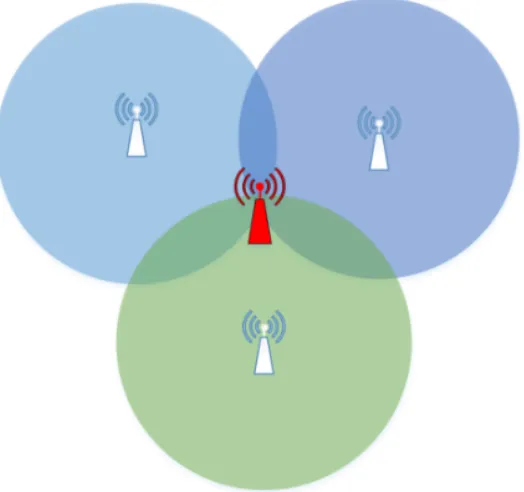
After determining the distance between the three anchors and tag using
two-way ranging, trilateration can then be applied to produce an estimated absolute
position. Trilateration in this case operates by using the points of intersection of
the three spheres, where the radius is equivalent to the received distance. Ideally,
this should give exactly two points of intersection since the vehicle platform is on
the ground, while the three anchors are elevated. In Fig. 2.1, the two points of
intersection would be one going into the page, and another one going out of the
page with equivalent distance from the center. However, only the 2D coordinates
are needed for this case since the vehicle platform will only be navigating on a 2D
map. If the height component is needed for other work, a fourth anchor will be
Figure 2.1: An ideal example diagram of trilateration for 2D positioning.
2.2
Inertial Measurement Unit
Nowadays, IMUs can come as small as the size of a Canadian quarter and are
referred to as microelectromechanical systems (MEMS). These MEMS can operate
with minimal power requirements and can fit into many other devices such as
cellphones, vehicles, and video game controllers. Cellphones can then be used
for tracking user movements such as steps, vehicle safety systems can respond
to sudden stops or movements, and video game controllers can use the IMU as
another way of controlling game movement. Thus, their ability to operate with fast
response times and accurate measurements make IMUs useful for this experiment.
2.2.1
Accelerometer
One of the measured values from the IMU is acceleration and measured in g, the gravity vector. Originally, a stationary IMU should always have a reading
fusion allows some IMUs to filter out the gravitational pull and only output the
linear acceleration that is needed for typical vehicle movements. More details
about the chosen IMU and its sensor fusion is discussed in Chapter 3.
2.2.2
Magnetometer and Gyroscope
The other two measured values from the IMU are magnetic field inµT and angular velocity in deg/s. The magnetometer responsible for the magnetic field detects the
magnetic poles of the Earth, and other magnetic objects nearby. However, it is best
to avoid changing the field around the magnetometer after calibration is done to
produce the best results. Ideally, if the magnetometer detects only the magnetic
poles of the Earth and is calibrated properly, it will provide the most accurate
readings of the true North direction. On the other hand, the gyroscope responsible
for the angular velocity measure the rotation about an axis. A representation of
gyroscope readings are useful for an airplane in flight as the airplane would need
to know its proper Euler angles to fly properly. In this case, the vehicle platform
only requires the rotation about one axis. However, the Euler angles can only be
as accurate as its original position as the angular velocity can only provide relative
orientation and not absolute orientation. More details regarding the magnetometer
and gyroscope can be found in Chapter 3.
2.3
Kalman Filter
The Kalman filter is a filtering technique commonly used for multiple sensors,
containing some noise or known variance, and fusing them together in an attempt
to achieve a more accurate measurement than one sensor alone. The noise is
usually represented as process noise, such as wind or something cause by the
sensor’s surrounding during operation, and known variance can be represented as
the measuring accuracy of the sensor given by its datasheet. One of its common
GPS or IPS in this case, with another sensor that can produce a relative location,
such as an IMU. The main requirements for the Kalman filter are that the sensor
measurements should have a Gaussian distribution, be a linear system, and must
be compared in the same measurement domain. Another feature that makes the
Kalman filter popular is that it is recursive, requiring only the last state and
present set of data measurements for its input, and allows it to be computed in
real-time [4].
2.3.1
Extended Kalman Filter
As mentioned previously, the Kalman filter is great for linear systems and
measure-ments in the same domain, but cannot properly predict nonlinear systems without
some modifications. As a result, the extended and unscented Kalman filters were
designed to deal with nonlinear systems. The UKF specializes in constant changes
where linearizing the data would cause worse prediction, such as differential
steer-ing when drivsteer-ing. If the data was to be linearized, the tangent of the curves would
not be a good representation of the actual turn. On the other hand, the EKF
specializes in linearizing the data and works best for the maneuverability of the
vehicle platform for this experiment. More details about the vehicle platform is
presented in Section 3.1.5.
Consequently, the EKF is used for this experiment and the acceleration received
from the IMU will be linearized and then fused with the positioning values
re-ceived from the UWB based IPS. Balzer provides a detailed implementation of
the Kalman filter using 2D acceleration and 2D position as input [5]. As such,
Balzer’s implementation is as follows.
First, the Kalman filter can be split into the prediction phase and the correction
phase. The prediction phase requires the state vector matrix to represent what
is being tracked, and the error covariance from the initial state uncertainty and
process noise covariance. Accordingly, the prediction phase can seen in Eq. 2.1
Projecting the state ahead.
xk+1 =Axk+Buk (2.1)
Projecting the error covariance ahead.
Pk+1 =APkAT +Q (2.2)
The state vector of the system is represented in Eq. 2.3.
xk = x y ˙ x ˙ y ¨ x ¨ y (2.3) where:
x: is the x-component of position
y: is the y-component of position ˙
x: is the x-component of velocity ˙
y: is the y-component of velocity ¨
x: is the x-component of acceleration ¨
y: is the y-component of acceleration
Next, the formal definition for motion is given by Eq. 2.4 with the dynamics of
the Egomotion, A and Eq. 2.5 after removing the control input, u.
xk+1 =
1 0 ∆t 0 1 2∆t
2 0
0 1 0 ∆t 0 12∆t2
0 0 1 0 ∆t 0
0 0 0 1 0 ∆t
0 0 0 0 1 0
0 0 0 0 0 1
·hxyx˙y˙x¨y¨
i
k (2.5)
Now, the measurement matrices based on acceleration from the IMU and position
from the UWB based IPS are represented by Eq. 2.6 and Eq. 2.7.
y=H·x (2.6)
y =
1 0 0 0 0 0
0 1 0 0 0 0
0 0 0 0 1 0
0 0 0 0 0 1
·x (2.7)
where:
x: is the state
H: is the measurement
Afterwards, the initial state uncertainty, P, measurement covariance, R and pro-cess noise covariance, Q can be modeled by Eq. 2.8, Eq. 2.9, and Eq. 2.10. The matrices are simplified with 0 on the non diagonals as the sensors used in this case
have independent variances. The measurement matrix, R, was also simplified to only four rows since only the x-component and y-component of acceleration and
P =
px 0 0 0 0 0
0 py 0 0 0 0
0 0 px˙ 0 0 0 0 0 0 py˙ 0 0 0 0 0 0 px¨ 0
0 0 0 0 0 py¨
(2.8) R =
rx 0 0 0 0 0
0 ry 0 0 0 0
0 0 0 0 rx¨ 0 0 0 0 0 0 ry¨
(2.9) Q=
px 0 0 0 0 0
0 py 0 0 0 0
0 0 px˙ 0 0 0 0 0 0 py˙ 0 0 0 0 0 0 px¨ 0
0 0 0 0 0 py¨
(2.10)
The Kalman filter can now enter the correction phase after measurements and
their corresponding covariance matrix, R, are received. Finally, the correction phase can be seen in Eq. 2.11, Eq. 2.12, and Eq. 2.13.
Computing the Kalman Gain.
Kk =PkHT(HPkHT +R)−1 (2.11)
Updating the estimate via measurement using zk.
Updating the error variance with measurement matrix, H, and identity matrix, I.
Pk= (I−KkH)Pk (2.13)
2.4
Robot Operating System
ROS is an open source meta-operating system that runs on Unix operating
sys-tems, such as Linux Ubuntu. Similar to a regular operating system, it can provides
low-level device control and message-passing between processes, but it is not
de-signed to be the main operating system of a device. Since ROS is open source,
it includes many online repositories from other organizations or community of
developers, including industrial applications [6]. As described in [7], “ROS
run-time graph is a peer-to-peer network of processes (potentially distributed across
machines) that are loosely coupled using the ROS communication infrastructure.
ROS implements several different styles of communication, including synchronous
RPC-style communication over services, asynchronous streaming of data over
top-ics, and storage of data on a Parameter Server.”
2.4.1
ROS Nodes, Topics, and Messages
ROS nodes are processes that usually does some computation and are able to
communicate with each other. Some examples for this experiment are one node
responsible for the IMU data, another node responsible for the UWB data, and
another node responsible for processing both sensor data. They can communicate
through the use of topics, RPC services, or a parameter server. In order for nodes
to communicate, a unique topic, service, or server name must be assigned by the
node. Afterwards, any node in the system can publish or subscribe to that topic
name. Publishing to a topic is similar to sending data to that topic name, while
subscribing is similar to receiving the data. Each topic must be assigned a proper
message structure, either custom built or one of the ROS messages. For example,
angular velocity, and orientation data. It is important to note that the node
publishing and subscribing to the topic must use the same message structure.
2.4.2
Navigation Stack
The navigation stack is a collection of ROS packages that receives input data
from certain sensors and outputs safe velocity commands to the vehicle [8]. A
ROS package is a method used by ROS in bundling software; thus, it can
con-tain multiple ROS nodes, a ROS-independent library, or other software of similar
use. These sensors include, but are not limited to, lidar, laser rangefinders, and
cameras. Furthermore, the navigation stack contains multiple ROS packages that
can be used together to achieve full autonomy. For example, planner packages
such as base local planner, dwa local planner, and global planner can be used for
pathfinding. The package map server will handle updates made to all maps, and
move base will handle movement of the robot. Fig. 2.2 shows an overview diagram
of how the navigation stack works [7].
Figure 2.2: An overview diagram of ROS topics and nodes for the navigation
stack.
2.5
Related Works
in manufacturing or warehouse management environments [9]. Ubisense is using
a system called ‘Smart Factory’ that helps manufacturers optimize efficiency with
the use of asset tracking [10]. Another industrial use is for navigating a robot for
painting a floor layout as mentioned in [11].
Similar indoor positioning systems include an UWB and MEMS based indoor
navigation for pedestrians. Through the use of multiple observation data such as
angles of arrival, time differences of arrival, accelerations, angular velocities, and
magnetic fields, Renaudin, Merminod, and Kasser were able to produce at best
position errors below 1 meter with a 0.1 meter variance [12]. Similarly, Evennou
and Marx studied an advanced integration of Wifi and inertial navigation systems
to produce a mean error of 2.56 meter using a Kalman filter, and mean error of
1.53 meter using a particle filter with an inertial navigation system [13].
Addition-ally, Yuan, Xiyuan, and Qinghua used an iterated EKF in forward data processing
of the Extended Rauch-Tung-Striebel smoothing to produce a position error of
3.50 -3.73cm [14]. Likewise, Jun, Guensler, and Ogle studied different methods of
GPS distance smoothing and concluded that the Kalman filter and their modified
Kalman filter produced better results than least squares spline approximation and
a Kernel-based smoothing method [15]. Yavari also studied UWB positioning with
LOS and NLOS conditions and produced at best an average positioning accuracy
of 10.97 cm and 51.96 cm, respectively [3].
ROS has also been helpful in research topics regarding indoor robotics. Foote
cre-ated the ROS tf library that allows the user to keep track of multiple coordinate
frames over time [16]. Furthermore, Marder-Eppstein et al. designed a robust
navigation system in a typical indoor office environment that had a robot
navi-gate itself for 26.2 miles without human intervention [17]. In addition, Garimort,
Hornung, and Bennewitz also designed navigation for a humanoid with dynamic
footstep plans [18]. This paper also accounts for the ability for humanoid robots
to step over certain obstacles compared to wheeled robots that would have to
Platform Hardware and Software
Implementation
3.1
Component Selection and Evaluation
This section explains why specific hardware and software components were used
for the experiment. As mentioned in Section 1.1, the motivation of this project
is to continue working on the Decawave UWB evaluation kit and its possible
applications as an accurate indoor positioning system. Accordingly, the Decawave
TREK1000 evaluation kit will be used for the positioning system and can be
seen in Fig. 3.1. Comparisons with other wireless positioning systems are further
discussed in [1]. Next, the software and programming language to be used was the
Figure 3.1: Decawave TREK1000 evaluation kit used as 3 anchors and 1 tag
configuration.
3.1.1
Software and Programming Language
Originally, the plan was to just write the entire project using a single Python
script since Python is easily accessible, large community for troubleshooting, and
large support for drivers and other libraries. Unfortunately, this could lead to
some bottleneck issues depending on the computer’s processor that is being used
and may not be as reliable when running real-time calculations. Fortunately, ROS
was found to be compatible with both C++ and Python language and allows for
multiple processes, or Python scripts, to run simultaneously and communicate
with each other. ROS communicates by sending structured messages using ROS
nodes and topics as mentioned in Section 2.4. Additionally, ROS already includes
built in sensor messages such as Odometry for positioning and IMU message for
IMUs. This was the major deciding factor for utilizing ROS for this platform.
Finally, ROS Indigo was chosen for being the latest long term support version
3.1.2
Master Computer
The master computer for this experiment does not have very high requirements
besides being compatible with Ubuntu 14 and ROS Indigo. Accordingly, a Lenovo
Yoga 2 Pro model was used with an Intel Core i5-4210 CPU @ 1.70 GHz x 4
processor with integrated graphics. It runs Ubuntu 14 64-bit with 8GB of RAM.
This computer was chosen as it was already owned, acts as a minimal requirement
for specifications, and the project did not need to do any known heavy computing.
3.1.3
Microcontroller
The microcontroller to be used for this experiment required it to be compatible
with Debian 8, have I2C bus lines, Wi-fi connectivity, USB port, and bonus for
having a readily available motor controller (this avoids creating a custom board
and leads to better scalability as it keeps all the header pins available). The
operating system must be Debian 8 as it is needed for the installation of ROS
Indigo, as chosen earlier in Section 3.1.1. Additionally, the I2C bus lines is for the
IMU or other future sensors, and the USB port is for the Decawave UWB tag, Wi-fi
adapter, or other future sensors. The two major candidates for the microcontroller
to be used were the Beaglebone Black or the Raspberry Pi 2 Model B as they are
both known to be compatible with running Debian.
The comparison of the technical specifications of the BBB and the Raspberry Pi 2
Model B can be seen in Table 3.1. The processing power of both microcontrollers
were relatively similar with a difference of only 100 MHz, so it was a major deciding
factor. However, the BBB only had half the RAM of the Raspberry Pi 2, but this
can be compensated by using a portion of the microSD card as a swap space to also
give it a RAM of 1GB. Furthermore, the BBB model had no integrated WLAN
adapter, but could also be compensated by using a low cost Wi-fi dongle. It was
also found that both microcontrollers are capable of running a Debian operating
system and both microcontrollers had support for a motor controller that can
microcontroller came down to the pin count and experience. The larger GPIO pin
count for the microcontroller ensured that the platform would be easily scalable
with multiple sensors for future use. Based on experience from past projects and
peers, the BBB seemed adequate enough for the experiment. As a result, the BBB
was chosen as the microcontroller to be used.
Table 3.1: BBB vs Raspberry Pi 2
Beaglebone Black Raspberry Pi 2 Model B
Price $ 84.31 $ 48.99
Processor 1 GHz 900 MHz
RAM 512 MB 1 GB
Wireless LAN Not included Integrated 802.11n
Power Source 5V @ 2A DC Jack 5V Micro-USB @ 2A
Pin count 92 (65 GPIO) 40 (26 GPIO)
Operating System
Debian compatible Debian compatible
Motor Controller
Seeed Motor Bridge Cape Adafruit DC Motor Hat
3.1.4
Inertial Measurement Unit
The IMU requirements for this experiment were to give an accurate measurement
of linear acceleration, magnetic field, and relative angular velocity. The linear
acceleration will be used in the EKF for predicting the relative position of the
vehicle, while the magnetic field and relative angular velocities will be used
to-gether in calculating the current heading of the vehicle. There were three IMUs
that were studied for this experiment: Xsens MTi 10-series [19], Adafruit 9-DOF
IMU Breakout [20], and Adafruit BNO055 Absolute Orientation Sensor [21].
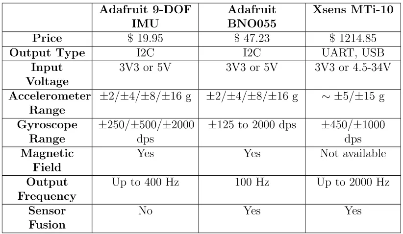
Table 3.2 shows a comparison of some specifications of each IMU. The compatible
output interfaces with the chosen microcontroller were USB or I2C and all three
IMUs were able to supply either interface. In addition, the input voltages for
all three IMUs could be provided by the BBB as well. Although the ranges for
the accelerometer and gyroscope values differ between the three IMUs, each IMU
can provide an acceptable operating range, (<5 g for linear acceleration, and <
seemed sufficient enough for the project, (<100 Hz should be able to provide real-time measurements). Unfortunately, the Adafruit 9-DOF IMU does not contain
its own sensor fusion output compared to the other two IMUs. Also, the Xsens
MTi-10 series lacks magnetic field readings and has a very steep price compared
to the two Adafruit IMUs. The magnetic field readings are needed in order for
the vehicle platform to determine its true North based on the magnetic poles. As
a result, the Adafruit BNO055 Absolute Orientation Sensor was the chosen IMU
in terms of performance and price compromise.
Table 3.2: Inertial Measurement Units Comparisons
Adafruit 9-DOF IMU
Adafruit BNO055
Xsens MTi-10
Price $ 19.95 $ 47.23 $ 1214.85
Output Type I2C I2C UART, USB
Input Voltage
3V3 or 5V 3V3 or 5V 3V3 or 4.5-34V
Accelerometer Range
±2/±4/±8/±16 g ±2/±4/±8/±16 g ∼ ±5/±15 g
Gyroscope Range
±250/±500/±2000
dps
±125 to 2000 dps ±450/±1000
dps Magnetic
Field
Yes Yes Not available
Output Frequency
Up to 400 Hz 100 Hz Up to 2000 Hz
Sensor Fusion
No Yes Yes
3.1.5
Vehicle Platform
The vehicle platform was assembled using aluminum parts as its chassis with four
separate DC motors to control each wheel. By being able to control the motors
separately, the vehicle platform will be able to rotate in place by having half of the
motors spin forward and the other half spin backward. Each DC motor was rated
at 0.263 N.m with a current of 0.52 A. Table 3.4 shows the other specifications for the vehicle platform. Additionally, plywood was used as platforms to hold
Table 3.3: Vehicle Specification
Wheel Diameter 120mm
Wheel Width 60mm
Body Length 270mm
Body Width 280mm
Motor Rated Voltage 12V DC
Motor Load Speed 100RPM
Motor Rated Speed 90RPM
Motor Gearbox Length 19mm
Motor Rated Current 0.52A
Motor Rated Torque 0.263N.m
Motor Maximum Torque 0.597N.m
platforms to be stacked on top. Plywood also makes it easier to drill through
compared to the sturdier aluminum chassis. Furthermore, a small plastic pipe
was attached to the side of the vehicle in order to elevate the IMU away from
the magnetic field disturbance produced by the DC motors. Accordingly, different
views of the vehicle platform can be seen in Fig. A.1, Fig. A.2 and Fig. A.3.
3.1.6
Power Supply
After choosing the BBB as the main microcontroller and its corresponding motor
controller, Seed Motor Bridge Cape, the power requirements for the platform are
5V @ 2A for the BBB and 12V DC for the motor controller. The BBB power must
be supplied through a 5.5 mm/2.1 mm DC barrel jack and must be able to handle currents of up to 2A, due to the power requirement for Wi-fi and other peripherals.
To satisfy the requirements, a custom built USB 2.0 A male to 5.5 mm/2.1 mm DC barrel jack connector was created using 18AWG wires. The 18AWG wires were
used to guarantee that up to 2A can be used for power transmission following
the AWG guide in [22]. As for the main power source for the BBB, a 20000mAh
portable battery pack with rated 2.4A output per USB port was purchased to
ensure that the BBB can operate with its peripherals properly. For the motor
controller, the 12V DC power supply will be used with PWM to control the speed
of the four separate DC motors. As a result, two sets of 12V NiMH rechargeable
Additionally, a set of Tamiya battery connector plugs and sockets were used to
connect the battery pack to the motor controller. The connections to the power
supplies can be seen in Fig. A.1 and Fig. A.2.
3.2
Device Specifications
In order for the vehicle platform to function properly, certain specifications must
first be met. Table 3.4 shows the specifications needed for the master PC and
the chosen microcontroller based on the previous components mentioned. Firstly,
the master PC and the BBB must both be connected to the same local network.
Internet is not necessary for this project to operate; however, the experiment setup
in this paper requires Internet to connect to ntp time servers to synchronize the
time between the master PC and the BBB. It is recommended to disable the devices
from automatically setting time from the Internet to ensure that the devices do
not try to connect to other time servers. This experiment uses the time servers of
the University of Windsor for time synchronization.
Table 3.4: Device Specifications
Master PC BBB
Power Computer dependent up to 10W at 5V
Wi-fi Yes Yes
Operating System Ubuntu 14 Debian 8
ROS Version Indigo Indigo
roscore Running Not running
ROS MASTER URI <IP ADDR>:11311 Master PC’s URI Network/IP Address xxx.xxx.xxx.1-254 xxx.xxx.xxx.1-254
Subnet Mask 255.255.255.0 255.255.255.0
IMU Not connected Connected via I2C 2 bus
Decawave UWB Tags Not connected Connected via USB
Moreover, the operating systems may vary for each device, but it must be
compat-ible with the selected ROS distribution. Roscore is used as the main process for
communication between ROS nodes and should be run on the master PC, while
the BBB should export the corresponding ROS Master URI to communicate
for providing an absolute position and the BNO055 IMU for providing linear
ac-celeration, magnetic field readings, and relative angular velocity. The UWB tag
is connected to the BBB via USB, while the IMU is connected via I2C 2 bus line
on the BBB. Accordingly, an overview of the connections can be seen in Fig. 3.2.
Figure 3.2: An overview diagram of the project connectivity.
3.3
Sensor Interface
This section explains the interface between the sensors and the BBB to receive
raw data for processing. However, the processing and application of filters will be
explained in greater detail in Chapter 4.
3.3.1
Ultrawideband
The UWB tag connected to the BBB via USB can be accessed using the Python
serial library. The initial code received from the past research work at the
Uni-versity of Windsor Wicip Lab used the ttyACM0 port at a baud rate of 9600 to
read the output of the UWB tag and store it in a text file. Then, another Python
text file. However, this method is not ideal for real-time applications since it
re-quires having to open and close the text file in every iteration. As a result, the
files were modified to work better for real-time calculations.
Instead of reading the output data from a text file, the trilateration calculations
were placed inside a function that takes multiple input parameters as seen in
Algorithm 1. The parameters, dist#, represent the three distance values between the UWB tag on the vehicle platform and the three stationary anchors. The
following x#, y# parameters are the coordinate pairs for the known positions of the UWB anchors. Finally, the function returns the absolute position of the
UWB tag as a set of tuples for further processing. This modification allows for the
trilateration function to be called in the same iteration that the distance values are
read without the need to open, write or read, and close a file object. Furthermore,
if the raw distance values or calculated coordinates need to be recorded for future
research work, a separate Python script can simply subscribe to the corresponding
ROS topic and not have to interfere with the real-time positioning calculations.
Algorithm 1 Trilateration Function
1: function trilat(dist0, dist1, dist2, x0, y0, x1, y1, x2, y2) . Calculates position using trilateration with received distance and anchor coordinates 2: Apply trilateration formula
3: return (x pose, y pose) 4: end function
3.3.2
Inertial Measurement Unit
Next, the Adafruit BNO055 sensor uses the I2C bus lines and includes a Python
library to help interface with the sensor [21]. The sensor can be powered via 3.3V or 5V and connected to the default I2C bus line of the BBB. Using Fig. B.2 as a
reference, P9 1-2 can be used as the common ground, P9 7-8 for 5V power supply,
and P9 19-20 for the corresponding I2C 2 bus line. However, the Python library
for the BNO055 defaults to the I2C 1 bus line, (which may be compatible with
older versions of Debian), and does not match the configuration of the BBB with
driver file to correctly match the appropriate I2C bus line for data to be read
properly. Fig. 3.3 shows the BNO055 breakout board and its relative size.
Figure 3.3: Adafruit BNO055 breakout board compared with an American
quarter as reference.
Afterwards, the Adafruit BNO055 sensor can provide multiple types of data,
in-cluding raw readings and sensor fused data. All data available from the sensor are
Euler angles for roll, pitch, yaw (in◦), orientation as a quaternion, sensor
tempera-ture (in◦C), magnetometer data (inµT), gyroscope data (in deg/s), accelerometer data (in m/s2), linear acceleration data (in m/s2), and gravity acceleration data
(in m/s2). For this experiment, the important data needed are Euler angles, linear
acceleration, magnetometer data, and gyroscope data. At first, the orientation as
a quaternion was supposed to be used to properly match the ROS IMU sensor
message structure. However, sending the quaternion orientation as a ROS
mes-sage would always throw an error that the values were not normalized, most likely
due to rounding limitations. As a result, the Euler angles were read instead and
then transformed into a quaternion orientation using the ROS transforms library.
Moreover, the linear acceleration is chosen for estimating the vehicle platform’s
position because the acceleration due to gravity is already filtered out, preventing
it from generating unnecessary noise. Lastly, the magnetometer and gyroscope
data are fused together to accurately track the current orientation of the vehicle
platform. The magnetometer allows for finding its orientation after power up,
while the gyroscope excels when there is magnetic field disturbance around the
Furthermore, the Adafruit BNO055 sensor also came with its own manual on how
to properly calibrate the acceleration, gyroscope, and magnetometer data [23].
Additionally, the calibrated registers can be saved after successful calibration to
avoid having to go through the physical calibration process again. Similar to
Section 3.3.1, the raw values before processing can also be recorded using the
same method without interfering with the rest of the program. It is worth noting
that this experiment is done in 2D only and only require the use of the x and y
linear acceleration.
3.4
Experimental Setup
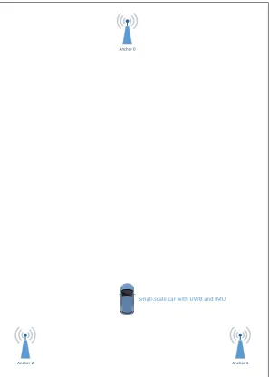
This section briefly explains the setup and scenario for the experiment. Figure 3.4
shows an overview diagram of the placement of the UWB anchors and the starting
point of the vehicle platform containing the UWB tag. The location for the tests
were done in the hallways outside the Wicip Lab. The floor is tiled and the tests
done avoids any major ramps or slants. It is important to note that the anchors are
elevated to a height of 1.5 m by using tripods, while the vehicle platform continues
to operate on ground level. Table 3.5 shows the respective anchor coordinates and
the output frequencies for the IMU and IPS used in the experiments. The IPS
frequency was kept constant throughout the experiments, but the IMU output data
frequencies were modified to study the process noise of the accelerometer. The
original output frequency of the accelerometer was at 30 Hz, but was concluded to
be too noisy to be useful in predicting position. As a result, the 30 Hz acceleration
values received were averaged over two different time windows for the tests. The
first set of tests took the average of acceleration values over 1/3 seconds resulting in a frequency output of 3 Hz, while the second set of tests took the average of
Anchor 0
Anchor 2 Anchor 1
Small-scale car with UWB and IMU
Figure 3.4: Experimental setup of experiment in the hallway (not to scale).
Table 3.5: Experiment Parameters
Parameter Value
Anchor 0 (2.196 m, 19.840 m) Anchor 1 (3.380 m, 0.000 m) Anchor 2 (0.620 m, 0.000 m) Anchor height 1.5m above ground IMU Frequency 1.0 - 3.0 Hz
Methodology and Description of
the Work
4.1
Position Estimation
The vehicle platform consists of two sensors that produces a position estimate: the
UWB based IPS and the IMU. Process for how each system estimates the position
can be found in Section 2.1 and Section 2.2. On the other hand, this section will
explain the data processing done in an attempt to improve the problems of the
current system.
4.1.1
Smoothing IPS
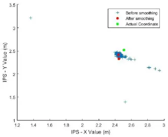
The first problem encountered was the measurement noise of the UWB tag when
stationary. After the navigation goal and path finding is done by the ROS
naviga-tion stack, it sends a safe velocity command to guide the vehicle platform through
the found path. However, every new measurement from the UWB tag would cause
the current position to change as seen by the multiple points in Fig. 4.1. As a
every new measurement, making it impossible to autonomously guide the vehicle
platform.
At first, a single threshold parameter was set to not update the current position
unless the new position received from the UWB tag was larger than the threshold.
However, this process made the results look more discrete (as the map only
up-dates when the vehicle moves past the threshold distance) rather than the desired
continuous feel of tracking. Another method attempted was calculating the
aver-age of the received measurements over 1 second, but this just resulted in delaying
the time the next position would change to every 1 second rather than 3.5 times a second.
Therefore, the proposed solution was to use a moving window average with a
de-sired threshold distance. By using a moving window average, the output frequency
of the data can continue to remain at 3.5 Hz and the only delay would be the initial time it takes to fill the window when starting. Calculating the average of the
win-dow also helps to mitigate some outliers during operation. Additionally, the use of
the threshold distance helps reduce the measurement noise by not accepting small
position changes. As a result, the average of the window would not be changed
unless the measurement values are large changes, which is more likely to happen
when the vehicle platform is in motion. The final result can be seen in Fig. 4.1,
where it drastically reduces the measurement noise to an acceptable stationary
position for consistent velocity commands.
Algorithm 2 Moving Window Average with Threshold Distance
1: procedure Smooth IPS(x pose, y pose) . Smoothens the output coordinates
2: if buf f er window! =window sizethen 3: append coordinates tobuf f er window
4: else if length(buf f er window) ==window size AND distance(new pose−
avg pose)> threshold distance then 5: delete oldestbuf f er window values 6: append new values tobuf f er window
7: end if
8: avg pose x= average ofx values in buf f er window
9: avg pose y = average of y values inbuf f er window
Figure 4.1: Plot comparing the output coordinates before and after
Algo-rithm 2.
4.1.2
Processing IMU Data
Fortunately, the Adafruit BNO055 sensor chosen for this experiment had its own
sensor fusion done by an on-board processor. As such, the fused data was able to
estimate the proper orientation of the vehicle platform accurately. However, the
problems that occurred during the tests were interpreting high output
frequen-cies of the linear acceleration, interpreting linear acceleration after turning, and
calibrating the linear acceleration to zero.
As mentioned previously in Section 3.4, the linear acceleration data received at
30 Hz made it very difficult to produce a good estimate of the vehicle platform’s
relative position. Accordingly, the IMU output was reduced to 3 Hz and 1 Hz in
an attempt to make the linear acceleration have a better prediction of the vehicle
platform’s position.
Secondly, the reference direction of the IMU when turning does not cause the
coordinate frames used for the experiment. For example, the base link frame
rep-resents the vehicle platform and the base imu reprep-resents the IMU. If the base link
frame (front of the vehicle platform) and the base imu (x-linear acceleration) are
both originally facing North and a 90◦ clockwise turn was made, the problem was
that the interpreted x-linear acceleration would cause the position to be updated
as moving in the North direction rather than East. The problem was solved by
using ROS transforms to properly track the rotational change of the base imu
rel-ative to the base link. Now, every time a linear acceleration value is received from
the base imu, the change in orientation is applied to the linear acceleration before
being interpreted by the base link frame.
Next, the measurements of the linear acceleration had to be further calibrated to
match its position on the vehicle. Although the Adafruit BNO055 sensor’s onboard
processor does a good job of filtering out acceleration due to gravity, there was still
some small acceleration values that were being read when the vehicle platform was
stationary. As a result, a calibration method was applied to correct the small linear
acceleration values being detected when the vehicle platform is stationary. The
calibration works by collecting linear acceleration values for the first few seconds
and determining the maximum, minimum and average values over the time period.
For this experiment, a calibration time of 4 seconds was found to be adequate in
determining the minimum and maximum values. During calibration, the vehicle
should remain stationary to best represent a zero acceleration scenario. After the
maximum, minimum and average values are recorded, all future values that are
between the minimum and maximum values return a value of 0m/s2. For values
outside of this range, the calibration method will return the difference of the value
and the average value from calibration. As a result, this calibration method should
avoid publishing most acceleration values while the vehicle platform is stationary.
Algorithm 3 shows the calibration function used for linear acceleration in the
x-direction. Likewise, the same method can be applied to the other dimensions as
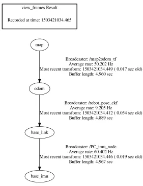
view_frames Result
base_link
base_imu
Broadcaster: /PC_imu_node Average rate: 60.402 Hz
Most recent transform: 1503421034.446 ( 0.019 sec old) Buffer length: 4.967 sec
odom
Broadcaster: /robot_pose_ekf Average rate: 9.205 Hz
Most recent transform: 1503421034.412 ( 0.054 sec old) Buffer length: 4.889 sec
map
Broadcaster: /map2odom_tf Average rate: 50.202 Hz
Most recent transform: 1503421034.449 ( 0.017 sec old) Buffer length: 4.960 sec
Recorded at time: 1503421034.465
Figure 4.2: ROS transform frames used for the experiment.
Algorithm 3 Calibrating IMU to zero out when stationary.
1: function sensor calibrate(x accel) .Returns 0 if linear acceleration is within the calibrated min/max.
2: if x accel >=xmin and x accel <=xmax then
3: return0.0
4: else
5: returnx accel−xavg
6: end if
4.1.3
Extended Kalman Filter
The EKF is a modification of the original Kalman Filter as previously described
in Section 2.3. In this experiment, the ‘robot pose ekf’ from the ROS navigation
stack was utilized. The ‘robot pose ekf’ has four possible inputs with the following
topic names: odom, imu data, vo, and gps. As for outputs, it publishes a topic
named ‘robot pose ekf/odom combined’ and a transformation between the odom
frame and base link frame. As described in [8], the ‘robot pose ekf’ uses the
relative pose differences rather than the absolute poses of the received data from
the sensor. For example, if the vehicle platform moves from coordinate position
(3, 4) to (3, 8), it is interpreted as a movement of 4 units rather than using the final
position of (3, 8). As more sensors are added into the ‘robot pose ekf’, it becomes
impossible to compare absolute position between different sensor reference frames.
Furthermore, the covariance of the sensors are used rather than the covariance
of the EKF pose for future calculations, as the EKF pose covariance would be
infinitely increasing as more sensor data is received. Lastly, the timing mentioned
in [8] explains that there must be a measurement from at least two different sensors
before it produces an output. After receiving the required measurement data, the
‘robot pose ekf’ produces an estimated position based on the latest time where
both sensor data is available. For sensor data that have different output rates,
interpolation is done in order to calculate the measurement at the earlier time.
For this experiment, the input data used were ‘imu data’, ‘vo’, and ‘gps’. The
‘imu data’ uses the ROS message structure for an IMU found in [8], while the
‘vo’and ‘gps’ both use the ROS message structure for Odometry. The ‘imu data’
receives a quaternion orientation, 3D angular velocity, and 3D linear acceleration,
each having its own 3x3 covariance matrix. A sample covariance matrix for the
‘imu data’ can be seen in Eq. 4.1. Note that since the variance in one direction
does not influence the other directions, only the diagonal have non-zero values.
Furthermore, since acceleration in the z-direction is not used, it should be given a
covariance matrix=
x 0 0 0 y 0 0 0 z
(4.1) where:
x: is the x-component for angular velocity, linear acceleration, or rotation
y: is the y-component for angular velocity, linear acceleration, or rotation
z: is the z-component for angular velocity, linear acceleration, or rotation Moreover, the ‘vo’ receives a 2D pose estimate equivalent to displacement
inte-grated from the linear acceleration, and the ‘gps’ receives a 2D pose estimate from
our UWB based IPS. Accordingly, both 2D pose estimates use the ROS
Odome-try message which follows a 3D pose structure with both position and orientation.
Thus, this message results in a 6x6 matrix and a similar covariance matrix can be
seen in Eq. 4.2. In order to publish only the 2D pose estimate, higher variance
values should be given for the z pose, x rot, y rot, and z rot since ‘vo’ and ‘gps’ cannot accurately measure these components.
covariance matrix=
xpose 0 0 0 0 0
0 y pose 0 0 0 0
0 0 z pose 0 0 0
0 0 0 xrot 0 0
0 0 0 0 yrot 0
0 0 0 0 0 zrot
(4.2) where:
xpose: is the x-coordinate for positioning
ypose: is the y-coordinate for positioning
zpose: is the z-coordinate for positioning
xrot: is the rotation about the x-axis
yrot: is the rotation about the y-axis
As mentioned earlier in Section 2.3, the covariance matrices have a major impact
on how the sensor data will be treated. Higher variances lead to a less trusted
sensor data, while lower variances will cause the EKF to trust the according sensor
data more. Therefore, these covariance matrices represent the measurement and
process noise for each sensor, and will need to be modified to achieve a desirable
Testings and Results
The values for the following tests were recorded by subscribing to the
correspond-ing ROS topic and storcorrespond-ing the values in a separate file, which was then plotted
by using MATLAB. This method ensures that the data logging process avoids as
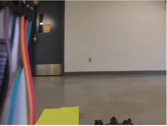
much interference with the real time processing of the data. Measured values were
recorded by attaching a small action camera on the vehicle platform and the use of
coloured markers on the floor as seen in Fig. 5.1. However, the start of recording
the test values and starting the camera were done manually so it may account for
some milliseconds in timing error. Lastly, the command sent to the vehicle
plat-form was a single ‘go forward’ command calculated to be about 0.23m/s, and was
Figure 5.1: Test markers as seen by the camera for known positions.
5.1
Preliminary Tests
The preliminary results seen in Fig.C.1, Fig. C.2, and Fig. C.3 were used as a
reference to determine how the ‘robot pose ekf’ would treat the initial covariance
matrices of Eq. 5.1 and Eq. 5.2.
displacement f rom imu=
0.001 0 0 0 0 0
0 0.001 0 0 0 0
0 0 99999 0 0 0
0 0 0 99999 0 0
0 0 0 0 99999 0
0 0 0 0 0 99999
displacement f rom ips=
0.00001 0 0 0 0 0
0 0.00001 0 0 0 0
0 0 99999 0 0 0
0 0 0 99999 0 0
0 0 0 0 99999 0
0 0 0 0 0 99999
(5.2)
5.2
Test using IMU Average Output at 3 Hz and
IPS Output at 3.5 Hz
It was observed that the linear acceleration with reference to the front and back
of the vehicle is not as reliable as the positioning from UWB. On the other hand,
the linear acceleration with reference to the side of the vehicle is more accurate,
especially since the vehicle is not able to move sideways. Therefore, the following
tests were completed by using a constant IPS covariance seen in Eq. 5.3 and a
varying covariance for the IMU as seen in Eq. 5.4, Eq. 5.5, and Eq. 5.6.
5.2.1
Test Run 1
First test with modified IMU covariance.
displacement f rom ips=
0.001 0 0 0 0 0
0 0.001 0 0 0 0
0 0 999999 0 0 0
0 0 0 999999 0 0
0 0 0 0 999999 0
0 0 0 0 0 999999
displacement f rom imu=
0.00001 0 0 0 0 0
0 0.1 0 0 0 0
0 0 999999 0 0 0
0 0 0 999999 0 0
0 0 0 0 999999 0
0 0 0 0 0 999999
(5.4)
Table 5.1: Test 1: IMU Output @ 3 Hz and IPS Output @ 3.5 Hz
Measured Values (meter)
IPS (meter) EKF (meter)
Start (2.153, 3.185) (2.039, 3.036) (2.039, 3.036)
Point 1 (2.129, 5.932) (2.165, 6.178) (1.977, 6.274) Point 2 (2.112, 7.859) (2.103, 8.087) (1.992, 8.450) Point 3 (2.089, 10.402) (1.757, 10.644) (2.012, 10.940)
End (2.053, 14.512) (1.316, 14.462) (1.972, 14.436)
Table 5.2: Test 1: Error in positioning using measured values.
IPS only error (meter) EKF error (meter)
Start 0.187 0.187
Point 1 0.249 0.374
Point 2 0.228 0.603
Point 3 0.411 0.544
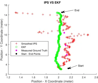
Position - X Coordinate (meter)
1.2 1.4 1.6 1.8 2 2.2 2.4 2.6
Position - Y Coordinate (meter)
2 4 6 8 10 12 14 16
IPS VS EKF
Smoothed IPS EKF
Measured Ground Truth Start - End Points
End
Start
Figure 5.2: Comparison of coordinate position before and after filtering for
Test 1.
Time elapsed (seconds)
0 10 20 30 40 50 60
Displacement - X Value (meter)
1.2 1.4 1.6 1.8 2 2.2 2.4
2.6 Displacement - X Direction VS Time
IPS only IMU only EKF
Measured Ground Truth Start - End Point
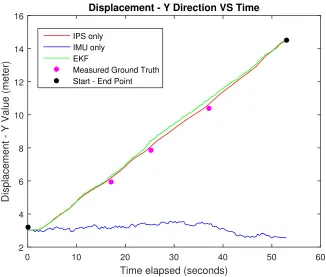
Time elapsed (seconds)
0 10 20 30 40 50 60
Displacement - Y Value (meter)
2 4 6 8 10 12 14
16 Displacement - Y Direction VS Time
IPS only IMU only EKF
Measured Ground Truth Start - End Point
Figure 5.4: Plot of y-coordinates versus time for real-time comparison.
5.2.2
Test Run 2
Second test with modified IMU covariance.
displacement f rom imu=
0.00001 0 0 0 0 0
0 0.01 0 0 0 0
0 0 999999 0 0 0
0 0 0 999999 0 0
0 0 0 0 999999 0
0 0 0 0 0 999999
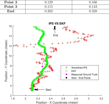
Table 5.3: Test 2: IMU Average Output @ 3 Hz and IPS Output @ 3.5 Hz Measured
Values (meter)
IPS (meter) EKF (meter)
Start (2.153, 3.185) (2.103, 3.056) (2.103, 3.056)
Point 1 (2.220, 5.932) (2.236, 6.199) (2.255, 6.146) Point 2 (2.267, 7.859) (2.378, 7.794) (2.312, 7.699) Point 3 (2.329, 10.402) (2.217, 10.375) (2.333, 10.259)
End (2.462, 15.830) (2.663, 15.815) (2.134, 15.815)
Table 5.4: Test 2: Error in positioning using measured values.
IPS only error (meter) EKF error (meter)
Start 0.138 0.138
Point 1 0.496 0.217
Point 2 0.129 0.166
Point 3 0.115 0.143
End 0.202 0.328
Position - X Coordinate (meter)
1.8 2 2.2 2.4 2.6 2.8 3 3.2
Position - Y Coordinate (meter)
2 4 6 8 10 12 14 16
IPS VS EKF
Smoothed IPS EKF
Measured Ground Truth Start - End Points End
Start
Figure 5.5: Comparison of coordinate position before and after filtering for
Time elapsed (seconds)
0 10 20 30 40 50 60 70
Displacement - X Value (meter)
1.8 2 2.2 2.4 2.6 2.8 3
3.2 Displacement - X Direction VS Time
IPS only IMU only EKF
Measured Ground Truth Start - End Point
Figure 5.6: Plot of x-coordinates versus time for real-time comparison.
Time elapsed (seconds)
0 10 20 30 40 50 60 70
Displacement - Y Value (meter)
0 2 4 6 8 10 12 14
16 Displacement - Y Direction VS Time
IPS only IMU only EKF
Measured Ground Truth Start - End Point
5.2.3
Test Run 3
Third test with modified IMU covariance.
displacement f rom imu=
0.00001 0 0 0 0 0
0 0.001 0 0 0 0
0 0 999999 0 0 0
0 0 0 999999 0 0
0 0 0 0 999999 0
0 0 0 0 0 999999
(5.6)
Table 5.5: Test 3: IMU Average Output @ 3 Hz and IPS Output @ 3.5 Hz
Measured Values (meter)
IPS (meter) EKF (meter)
Start (2.153, 3.185) (2.022, 3.006) (2.022, 3.006)
Point 1 (2.114, 5.932) (2.088, 5.454) (2.042, 5.252)
Point 2 (2.086, 7.859) (2.109,7.059) (2.066, 6.800)
Point 3 (2.049, 10.402) (2.145, 9.286) (2.116, 8.886) End (1.973, 15.751) (2.049, 15.745) (1.662, 15.744)
Table 5.6: Test 3: Error in positioning using measured values.
IPS only error (meter) EKF error (meter)
Start 0.222 0.222
Point 1 0.479 0.684
Point 2 0.800 1.059
Point 3 1.120 1.517
Position - X Coordinate (meter)
1.2 1.4 1.6 1.8 2 2.2 2.4 2.6
Position - Y Coordinate (meter)
2 4 6 8 10 12 14 16
IPS VS EKF
Smoothed IPS EKF
Measured Ground Truth Start - End Points
End
Start
Figure 5.8: Comparison of coordinate position before and after filtering for
Test 3.
Time elapsed (seconds)
0 10 20 30 40 50 60 70
Displacement - X Value (meter)
1.2 1.4 1.6 1.8 2 2.2 2.4
2.6 Displacement - X Direction VS Time
IPS only IMU only EKF
Measured Ground Truth Start - End Point
Time elapsed (seconds)
0 10 20 30 40 50 60 70
Displacement - Y Value (meter)
2 4 6 8 10 12 14
16 Displacement - Y Direction VS Time
IPS only IMU only EKF
Measured Ground Truth Start - End Point
Figure 5.10: Plot of y-coordinates versus time for real-time comparison.
5.3
Test using IMU Output at 1 Hz and IPS
Output at 3.5Hz
This section uses the same parameters as Section 5.2, but the IMU average
out-put is reduced to 1 Hz. Thus, the following test uses the same covariances as
Eq. 5.3 and Eq. 5.4. Further tests were also done with Eq. 5.5 and Eq. 5.6, but
were excluded due to the results being inconsistent; thus, they were considered
as outliers. As seen in Fig. 5.13, the lower output rate of the IMU produced a
reasonable displacement until about the 25 second mark, where the displacement
no longer became reliable. However, it can also be observed that once the vehicle
stopped around the 55 second mark, the displacement values began to flat line as