Performance Analysis of Elaborated Round Robin Scheme by Linear Data Model

(1)

Performance Analysis of Elaborated Round

Robin Scheme by Linear Data Model

Manish Vyas1, Dr. Saurabh Jain2

1

Sr. Assistant Professor, Acropolis Institute of Management Studies and Research, Indore, India

2

Associate Professor, ShriVaishnav Institute of Computer Application, Indore, India

ABSTRACT: Processor scheduling involves execution of pending processes in most efficient way. Ultimate performance of system depends on scheduling algorithms.In present scenario recent technology has increased complexity of processing, as computing come to be distributed and parallel. Due to this job scheduling is get complex in this environment. Any processor is said to be optimally performing if it has a higher throughput, low waiting time, low turnaround time, and less number of context switches for the processes ready for execution. As scheduler is key component hence to achieve its optimum usage, core stress is set on all the above factors during designing of various scheduling schemes.In this paper, a scheduling scheme is proposed by elaborating round robin scheme. Where CPU transitionis represented over more than one state through some particular strategy including waiting state where scheduler may get idle. Analysis of data values is done through a probabilistic linear data model and simulation study in terms of graphical representation is made for assessment of proposed scheme.

KEYWORDS: Process scheduling, Data model, Transition diagram, Rest state, Transition probability matrix, Simulation.

I. INTRODUCTION

In multiprocessing environment, the approach of dispatching processes to CPU is called process scheduling. Its main purpose is to execute processes in a way that system objectives such as response time, throughput and processor’s efficiency can be achieved. Scheduling bring up a set of strategies and mechanisms which regulate the order of work performed by system.To enhance scheduler performance, various technologically advanced scheduling algorithms are implemented which are having organized steps. Some algorithms are designed as an extension to usual algorithm where random behavior of scheduler might undertake over different transition states. And various comparable scheduling schemes may be proposed.

II. RELATED WORK

(2)

A finest time quantum is used for improving the performance of shortest remaining burst round robin algorithm by [13]. [14] Gives self-adjustment round robin algorithm by dynamic time quantum approach. For effective processing various scheduling schemes are available [3],[4].Some useful contributions in improving CPU utilization like process management, process scheduling & inter process communication are due to [5],[6].

In this paper we proposed a scheduling scheme by elaborating round robin scheme with some specific strategy. The transition of scheduler can remain on same process or move to next process after completion of allotted time quantum. Schemeis evaluated through simulation study. Linear data values based Markov chain model is used for exploration of transition probabilities. Suggested schemeisanalyzed on the basis of scheduler movement.

III. MARKOV CHAIN

A stochastic process is collection of random variables {Xn}, which develops in time according to probabilistic rules

where Xn will depend on earlier values of the process Xn−1,Xn−2,…... The collection of all these random variables is

called stochastic process.

A Stochastic process will satisfy Markov property, if the present state Xk is independent of past states ( Xk−1,Xk−2, Xk−3,

... , X1 ) i.e. state of a system at time t+1 depends only on its state at time t. Markov Process is a stochastic model that

has Markov property.

Definition: The stochastic process Xn, (n=0, 1, 2…) is called Markov chain if, for j, k, j1,…jn-1 € N or any subset of I,

Pr{ Xn = k / Xn –1 = j , Xn –2 = j1 ,….,X0 = jn – 1}

= Pr{Xn= k / Xn – 1 = j} =pjk

Transition Probability Matrix: The transition probabilities pjksatisfy

pjk0,





1

k jk

p

for all j.

These probabilities may be written in the matrix form

P =

This is called the transition probability matrix of the Markov chain. P is a stochastic matrix, i.e. a square matrix with

non-negative elements and unit row sums.

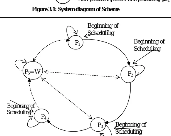
IV. REGULATED TRANSITION BASED MULTI PROCESS SCHEDULING SCHEME

In this scheme four processes P1, P2, P3 and P4are considered in ready queue for executionalong with one more state

P5as rest state.For processing, time quantum is decided.The schemedesigned under Regulated Transitionwhere

scheduler can pick any of process from P1, P2, P3 and P4 in beginning with initial probabilities as pr1,pr2, pr3,

pr4respectively.After completion of allotted time quantum, scheduler can move to next process state or can continue at

same state. P5 is rest or idle state where random transition of scheduler may occur from any of process Pi.

Scheduler continues within these states until all processes get finished.If any process gets complete within allotted time quantum then it eradicate from ready queue otherwise it remains in waiting queue and wait for next quantum to allot for its processing.After completion of time quantum, scheduler assign next quantum to next process and it continues till all processes gets completed.

... ... ... ...

... S S S

.

33 32 31

23 22 21

13 12 11

 n

X

(3)

P1

P2

P3

P4

P5= W

Beginning of Scheduling

Beginning of Scheduling Beginning of

Scheduling

Figure 3.2: Transition diagram of Scheme

a. Markov Chain Model On Multi Process Scheduling Scheme

Consider



X

 n

,

n



1 

as Markov chain where

X

 n is scheduler state at

n

th time quantum. State space for random variable X may P1, P2, P3, P4and P5. Initial probabilities for these stateswill be,

Where







4

1 4 3 2

1

i i

pr

P5

Xn

Scheduler

P1

P2

P3

P4

New process P1 enters with probability pr1

pr1

pr2

pr3

pr4

Figure 3.1: System diagram of Scheme

Beginning of Scheduling

 





 





 





 





 







     

 

 

0 P X p

pr P X p

5 0

4 4 0

3 3 0

2 2 0

(4)

The transition probability matrix will be,

Unit step transition probability matrix for

X

 n under scheme –I is

Remark 4.1.1: Defining an Indicator function Lij(for i, j=1,2,3,4,5) such that,

Lij = 0 when (i=1, j=3,4), (i=2, j=1,4), (i=3, j=1,2), (i=4, j=1,2,3)

Lij = 1 otherwise

The state probabilities after first quantum will be,

55 54 53 52 51 5 45 44 43 42 41 4 35 34 33 32 31 3 25 24 23 22 21 2 15 14 13 12 11 1 5 4 3 2 1

S

P

S

P

S

P

S

P

S

P

X

(n)

(n – 1)

(5)

 





 





 





 





 





                                                                                                                                                                    



m5 m5 kl kl 5 1 l 5 1 k 5 1

j jk jk

4

1

i i ij ij

5 1 m 5 n m4 m4 kl kl 5 1 l 5 1 k 5 1

j jk jk

4

1

i i ij ij

5 1 m 4 n m3 m3 kl kl 5 1 l 5 1 k 5 1

j jk jk

4

1

i i ij ij

5 1 m 3 n m2 m2 kl kl 5 1 l 5 1 k 5 1

j jk jk

4

1

i i ij ij

5 1 m 2 n m1 m1 kl kl 5 1 l 5 1 k 5 1

j jk jk

4

1

i i ij ij

5 1 m 1 n .L .S ... . L . .S L . S . L . .S pr ... P X p .L .S ... . L . .S L . S . L . .S pr ... P X p .L .S ... . L . .S L . S . L . .S pr ... P X p .L .S ... . L . .S L . S . L . .S pr ... P X p .L .S ... . L . .S L . S . L . .S pr ... P X p

Similarly state probabilities after the Second quantum will be

Generalized expressions for n time quantum are :

V. SIMULATION STUDY

By the means of simulation study scheduling scheme can be studied and analyzed forthis a linear data model is used

under Markov chain.State transition probabilities are obtained in linear order. Thematrix of data model is as,

(6)

As scheduler can pick any of process in the beginning, hence initial probabilities of processes will be pr1=0.25, pr2

=0.25, pr3=0.25, pr4=0.25 and pr5=0. Graphical analysis on the basis of Data obtained in the form of element transitional

probability matrices as,

Case 1: when a = 0.010

(a = 0.010, d = 0.002) (a = 0.010, d = 0.004)

(a = 0.010, d = 0.006) (a = 0.010, d = 0.008)

Case 2: when a = 0.012

(a = 0.012, d = 0.002) (a = 0.012, d = 0.004)

(a = 0.012, d = 0.006) (a = 0.012, d = 0.008)

0 0.5 1

1 3 5 7 9 11 13

P1 P2 P3 P4 P5

0 0.2 0.4 0.6 0.8 1

1 3 5 7 9 11 13

P1 P2 P3 P4 P5

0 0.5 1

1 3 5 7 9 11 13

P1 P2 P3 P4 P5

0 0.5 1

1 3 5 7 9 11 13

P1 P2 P3 P4 P5

0 0.5 1

1 3 5 7 9 11 13

P1 P2 P3 P4

0 0.2 0.4 0.6 0.8

1 3 5 7 9 11 13

P1 P2 P3 P4

0 0.2 0.4 0.6 0.8

1 3 5 7 9 11 13

P1 P2 P3 P4 0

0.5 1

(7)

Case 3: when a = 0.014

(a = 0.014, d = 0.002) (a = 0.014, d = 0.004)

(a = 0.014, d = 0.006) (a = 0.014, d = 0.008)

Case 4: when a = 0.016

(a = 0.016, d = 0.002) (a = 0.016, d = 0.004)

(a = 0.016, d = 0.006) (a = 0.016, d = 0.008)

0 0.5 1

1 3 5 7 9 11 13

P1 P2 P3 P4 P5

0 0.2 0.4 0.6 0.8 1

1 3 5 7 9 11 13

P1 P2 P3 P4 P5

0 0.2 0.4 0.6 0.8

1 3 5 7 9 11 13

P1 P2 P3 P4 P5

0 0.2 0.4 0.6 0.8

1 3 5 7 9 11 13

P1 P2 P3 P4 P5

0 0.5 1

1 3 5 7 9 11 13

P1 P2 P3 P4 P5

0 0.5 1

1 3 5 7 9 11 13

P1 P2 P3 P4

0 0.5 1

1 3 5 7 9 11 13

P1 P2 P3 P4

0 0.5 1

1 3 5 7 9 11 13

(8)

Case 5: when a = 0.018

(a = 0.018, d = 0.002) (a = 0.018, d = 0.004)

(a = 0.018, d = 0.006) (a = 0.018, d = 0.008)

VI. CONCLUSION

In this scheme,although initial probability of rest state is higher, but if time scale rises with origin then there is decrement in probability of P5 while increment in remaining all process states. At higher end P4 get higher probability with increase in P1, P2 and P3 also. This scheme shows stability pattern of system where probability of rest state is not much more than that of others. Here state probabilities increases for change in pattern of time quantum with decrement in probability of rest state. This scheduling scheme can be beneficial for scheduling.

Concluding towards analysis by considering probability based linear data model, it can be stated that the proposed scheduling schemecan be beneficial for job processing in proficient manner with reducing probability of rest state.

REFERENCES

1. E. Parzen (2015): Stochastic Process, Holden– day, Inc. San Francisco, California 2. J. Medhi (2010): Stochastic processes, , Wiley Limited Third Edition (Reprint) 3. Silberschatz, Galvin and Gagne (2009): Operating systems concepts, Eighth Ed., Wiley

4. A. Tanenbaum and A.S. Woodhull (2009): Operating System: Design and Implementation, third Ed., Prentice Hall of India Private Limited, New Delhi

5. W. Stalling (2004): Operating Systems, fifth Ed., Pearson Education, Singapore, Indian Ed., New Delhi 6. S.Haldar (2009): Operating Systems, Pearson Education, India

7. S.R. Chavan and P.C. Tikekar (2013): An Improved Optimum Multilevel Dynamic Round Robin Scheduling Algorithm, International Journal of Scientific & Engineering Research, Volume 4, Issue 12

8. B. SukumarBabu, N. NeelimaPriyanka and Dr. P. Suresh Varma (2012): Optimized Round Robin CPU Scheduling Algorithm, International Journal of Computer Applications (IJCA)

9. S.N. Shah and A. Mahmood Oxley(2009): Hybrid Scheduling and Dual Queue Scheduling ,IEEE Conference,978-1-4244-4520-2/09

10. D. Shukla and S. Jain (2008): A General Class of Round Robin Scheduling Schemes Under Markov Chain Model, The Next International Conference on Mathematics and Computer Science, ICMCS-08, pp. 62-70

11. M. Mishra and A.K. Khan (2012): An Improved Round Robin CPU Scheduling Algorithm, Journal of Global Research in Computer Science, Volume 3, No. 6

12. A. Abdulrahim, S. E. Abdullahi and J.B. Sahalu (2014): A New Improved Round Robin (NIRR) CPU Scheduling Algorithm, International Journal of Computer Applications, Volume 90, No. 4

13. A. Jamal and A. Zubair (2012): A Varied Round Robin Approach using Harmonic Mean of the Remaining Burst Time of the Processes, International Journal of Computer Applications, 3rd International IT Summit Confluence 2012 - The Next Generation Information Technology

0 0.5 1

1 3 5 7 9 11 13

P1 P2 P3 P4 P5

0 0.5 1

1 3 5 7 9 11 13

P1 P2 P3 P4

0 0.5 1

1 3 5 7 9 11 13

P1 P2 P3 P4

0 0.5 1

1 3 5 7 9 11 13

(9)

14. R. Jaiswal, K. Geeta and R. Mohan (2013): An Intelligent Adaptive Round Robin (IARR), Scheduling Algorithm for Performance Improvement in Real Time Systems, Proc. of Int. Conf. on Advances in Mechanical Engineering, AETAME

15. P. S. Varma (2013):A Finest Time Quantum For Improving Shortest Remaining Burst Round Robin (SRBRR) Algorithm, Journal of Global Research in Computer Science, vol. 04 , no. 03