University of Windsor University of Windsor
Scholarship at UWindsor
Scholarship at UWindsor
Electronic Theses and Dissertations Theses, Dissertations, and Major Papers
2011
The effect of weather on speed reduction on a freeway and air
The effect of weather on speed reduction on a freeway and air
pollutant dispersion pattern near the freeway
pollutant dispersion pattern near the freeway
Van Nguyen
University of Windsor
Follow this and additional works at: https://scholar.uwindsor.ca/etd
Recommended Citation Recommended Citation
Nguyen, Van, "The effect of weather on speed reduction on a freeway and air pollutant dispersion pattern near the freeway" (2011). Electronic Theses and Dissertations. 86.
https://scholar.uwindsor.ca/etd/86
The effect of weather on speed reduction on a freeway and air pollutant dispersion pattern
near the freeway
by
Van Nguyen
A Thesis
Submitted to the Faculty of Graduate Studies
through Civil and Environmental Engineering
in Partial Fulfillment of the Requirements for
the Degree of Master of Applied Science at the
University of Windsor
Windsor, Ontario, Canada
2011
The effect of weather on speed reduction on a freeway and air pollutant dispersion pattern
near the freeway
by
Van Nguyen
APPROVED BY:
______________________________________________ Dr. William Anderson
Department of Political Science
______________________________________________ Dr. Rajesh Seth
Department of Civil and Environmental Engineering
______________________________________________ Dr. Chris Lee, Co-Advisor
Department of Civil and Environmental Engineering
______________________________________________ Dr. Iris Xiaohong Xu, Advisor
Department of Civil and Environmental Engineering
______________________________________________ Dr. Hanna Maoh, Chair of Defense
Department of Civil and Environmental Engineering
DECLARATION OF ORIGINALITY
I hereby certify that I am the sole author of this thesis and that no part of this thesis
has been published or submitted for publication.
I certify that, to the best of my knowledge, my thesis does not infringe upon anyone’s copyright nor violate any proprietary rights and that any ideas, techniques,
quotations, or any other material from the work of other people included in my thesis,
published or otherwise, are fully acknowledged in accordance with the standard
referencing practices. Furthermore, to the extent that I have included copyrighted material
that surpasses the bounds of fair dealing within the meaning of the Canada Copyright Act,
I certify that I have obtained a written permission from the copyright owner(s) to include
such material(s) in my thesis and have included copies of such copyright clearances to my
appendix.
I declare that this is a true copy of my thesis, including any final revisions, as
approved by my thesis committee and the Graduate Studies office, and that this thesis has
ABSTRACT
This paper examines the variations in traffic speed and the dispersion pattern of
NOx produced from traffic in clear, rainy and snowy weather conditions. The data used for
the analysis include weekday hourly traffic count of 193 days in 1998 on Gardiner
Expressway, Toronto, Ontario, and the coincide 193 meteorology days. The ordered
logistic regression model was used to identify the relationships between speed reduction
and various factors. The EPA emission factor model and AERMOD were used to predict
NOx concentrations using traffic volumes and meteorology data.
Analysis of speed reduction shows precipitation, hour of day, snowy condition and
seasons reduce speed. The predicted dispersion show NOx concentration was high in clear
weather condition compared to adverse weather condition due to higher traffic volumes
and higher emissions. However, in snowy weather condition, wind speed had more
DEDICATION
To my beloved grandparents for their faith and unconditional love in me.
To my parents, Hung and Thu Nguyen, for their hard work keeping me in school.
To my sister, Janet: my first teacher.
Lastly to Trinh, my guidance and supporter through this journey.
ACKNOWLEDGEMENTS
I would like to take this opportunity to sincerely thank my supervisor, Dr. Iris
Xiaohong Xu and Dr. Chris Lee for their continuous support, assistance, guidance, and
constructive evaluations throughout the course of my graduate studies. I have learned a
great deal working with both. This thesis would not have been possible without their
inspirational guidance. I would also like to thank my thesis committee of Dr. Rajesh Seth
and Dr. William Anderson for their constructive inputs and advice.
I would also like to express thanks to my friends as well as colleagues at the
University. A very special thanks to Mr. Hassan Mohseni for helping me extracted the
Gardiner Expressways road profile in ArcGIS, providing the Matlab coding used to
discretize the road coordinates, and providing technical assistance in AERMOD modeling.
Special thanks to Mr. Udoka Nwaesei for helping with the traffic incident logs processing.
A special thanks to the City of Toronto in providing the traffic data and the
percentage of different vehicles on Gardiner Expressway.
The financial support for this thesis research partially provided by National
TABLE OF CONTENTS
DECLARATION OF ORIGINALITY ... iii
ABSTRACT ... iv
DEDICATION ...v
ACKNOWLEDGEMENTS ... vi
LIST OF TABLES ... ix
LIST OF FIGURES ...x
CHAPTER I. INTRODUCTION 1.1 OVERVIEW ...1
1.2 RESEACH OBJECTIVES ...2
1.3 ORGANIZATION OF THESIS ...2
II. REVIEW OF LITERATURES 2.1 WEATHER CONDITIONS, VEHICULAR SPEED AND VOLUME ...4
2.1.1 EFFECT OF WEATHER ON SPEED 2.1.2 EFFECT OF WEATHER ON TRAFFIC VOLUME 2.1.3 EFFECT OF WEATHER ON EMISSIONS FROM TRAFFIC 2.2 DISPERSION OF AIR POLLUTANTS FROM TRAFFIC ...10
2.3 SUMMARY ...13
III. DESCRIPTION OF DATA AND STUDY SITE 3.1 STUDY SITE AND DATASETS ...14
3.2 TRAFFIC DATA ...15
3.2.1 WEEKDAY TRAFFIC 3.2.2 INCIDENT LOGS 3.3 WEATHER DATA ...18
3.3.1 HOURLY WEATHER CONDITIONS FOR TRAFFIC ANALYSIS 3.3.2 METEOROLOGICAL DATA USED FOR DISPERSION MODELING IV. METHODOLOGY - TRAFFIC ANALYSIS 4.1 NORMAL SPEED PROFILES ...22
4.2 PRECIPITATION AND VISIBILITY ...23
4.3 DAYLIGHT CONDITION ...24
4.4 SPEED REDUCTION ...24
4.5 STATISTICAL METHODS ...25
4.5.1 CHI-SQUARE TEST 4.5.2 LOGISTIC REGRESSION: ORDERED REGRESSION MODEL 4.6 VARIABLE CLASSIFICATIONS ...28
V. RESULTS OF TRAFFIC ANALYSIS 5.1 SPEED DISTRIBUTION ...29
5.2 VOLUME DISTRIBUTION ...30
5.4 RELATIONSHIP OF WEATHER AND SEASON WITH SPEED
- RESULT OF CHI-SQUARE TEST ...40
5.5 RELATIONSHIP OF WEATHER AND SEASON WITH SPEED REDUCTION- RESULT OF CHI-SQUARE TEST ...45
5.6 ORDERED LOGISTIC REGRESSION...48
5.7 SUMMARY ...50
VI. METHODOLOGY – DISPERSION MODELLING 6.1 AERMOD MODELING ...51
6.1.1 METEOROLOGY DATA 6.1.2 EMISSION FACTOR 6.1.3 EMISSION RATE 6.2 SIMULATION DESIGN ...55
VII. RESULTS OF POLLUTANT DISPERSION 7.1 COMPARISON BETWEEN CLEAR WEATHER CONDITIONS VS. SNOW AND RAIN CONDITIONS ...59
7.2 COMPARISON BETWEEN CLEAR WEATHER CONDITIONS VS. CONDITION WITH SNOWY AND CLEAR AND RAINY AND CLEAR CONDITIONS ...63
7.3 COMPARISON BETWEEN DAYTIME AND NIGHTTIME CONDITON IN RAIN AND CLEAR AND SNOW AND CLEAR CONDITION. ...66
7.4 SUMMARY ...59
VIII. CONCLUSIONS AND RECOMMENDATIONS REFERENCES ...79
APPENDICES A. VISUAL BASIC CODING ...85
B. BSTATISTICAL ANALYSIS CODING ...92
C. SAS OUTPUTS ...94
D. RECEPTORS COORDINATES ...149
LIST OF TABLES
Chapter 2:
Table 2- 1. Speed reduction during rain and snow condition. (Source: Ibrahim and Hall,
1994) ... 4
Table 2- 2. Speed reduction based on road surfaces. (Source: FHWA, 1977) ... 6
Table 2- 3. Volumereduction due to snowstorm. (Source: Hanbali and Kuemmel, 1992) 7 Table 2- 4. Summary of Dispersion Models (Source: Table from Peirce et al, 2004) ... 12
Chapter 3: Table 3- 1. Raw data of speed and traffic volume on January 2nd, 1998. (Source: Toronto Traffic Operation Office Center, 2010) ... 17
Table 3- 2. Example of weather condition. (Source: Toronto Traffic Operation Office Center , 2010)... 19
Table 3- 3. Sample pre-processed upper air file. (Source: MoE, 2010) ... 20
Table 3- 4. Sample pre-processed surface file. (Source: EC, 2010) ... 21
Table 3- 5. Summary of data obtained from all sources ... 21
Chapter 4: Table 4- 1. Classifications of Variable for analysis ... 28
Chapter 5: Table 5- 1. Number of total non-recurrent incidents by season ... 34
Table 5- 2. Parameters estimation of the ordered logistic regression model (westbound) 49 Table 5- 3. Parameters estimation of the ordered logistic regression model (eastbound) 50 Chapter 6: Table 6- 1. Calculated NOx emission factors from EPA and the City of Toronto. ... 53
Table 6- 2. Model setup parameters for AERMOD simulation. ... 56
Table 6- 3. Simulation Design ... 58
Chapter 7: Table 7- 1. Wind speed and directions in rain, snow, and clear conditions... 73
Table 7- 2. Emission and Concentration ratios ... 73
LIST OF FIGURES
Chapter 2:
Figure 2- 1. NOx and CO emission produced from traffic in different speed. (Source:
FHWA, 2011) ... 8
Figure 2- 2. NOx emission from traffic in different speed and vehicle composition (Source: The Department of Transport, England, U.K, 2005) ... 8
Figure 2- 3. VOC, NOx and CO emission for car and trucks. (Source: FHWA, 2011) ... 9
Chapter 3: Figure 3- 1. Map of Gardiner Expressway, Toronto, ON. (Source: Base map by Google, 2011) ... 14
Figure 3- 2. Traffic stations along Gardiner Expressway. (Source: Lee et al., 2002) ... 16
Figure 3- 3. Sample of incident log for December 2, 1998. (Source: Toronto Traffic Operation Office Center10) ... 18
Chapter 4: Figure 4- 1. Process flowchart of all data ... 23
Figure 4- 2. Hourly variation in speed reduction on April 30, 1998 ... 25
Chapter 5: Figure 5- 1. Westbound speed distribution for 1998 ... 29
Figure 5- 2. Eastbound speed distribution for 1998 ... 30
Figure 5- 3. Westbound volume distribution for 1998 ... 31
Figure 5- 4. Eastbound volume distribution for 1998 ... 31
Figure 5- 5. Westbound volume distribution for 399 hours of clear weather condition ... 32
Figure 5- 6. Westbound volume distribution for 399 hours of adverse weather condition ... 32
Figure 5- 7. Eastbound volume distribution for 399 hours of clear weather condition .... 33
Figure 5- 8. Eastbound volume distribution for 399 hours of clear weather condition .... 33
Figure 5- 9. Winter Normal Speed Profile in westbound direction. ... 34
Figure 5- 10. Spring Normal Speed Profile in westbound direction... 35
Figure 5- 11. Summer Normal Speed Profile in westbound direction. ... 35
Figure 5- 12. Fall Normal Speed Profile in westbound direction. ... 36
Figure 5- 13. Variations in speed profiles for westbound direction ... 36
Figure 5- 14. Winter Normal Speed Profile in eastbound direction. ... 37
Figure 5- 15. Spring Normal Speed Profile in eastbound direction. ... 38
Figure 5- 16. Summer Normal Speed Profile in eastbound direction. ... 38
Figure 5- 17. Fall Normal Speed Profile in eastbound direction. ... 39
Figure 5- 18. Variations in speed profiles for eastbound direction. ... 39
Figure 5- 19. Relationship between speed and lighting.Result of Chi-square test, relationship is significant at p < 0.01 ... 41
Figure 5- 22. Relationship between speed and visibility. Result of Chi-square test,
relationship is significant at p < 0.1 ... 43 Figure 5- 23. Relationship between speed and season. Result of Chi-square test,
relationship is significant at p < 0.1 ... 43 Figure 5- 24. Relationship between volume and season for westbound and eastbound
direction. ... 44 Figure 5- 25. Relationship between speed and weather conditions. Result of Chi-square
test, relationship is significant at p < 0.1 ... 45 Figure 5- 26. Relationship between speed reduction and lighting. Result of Chi-square
test, relationship is significant at p <0.1 ... 46 Figure 5- 27. Relationship between speed reduction and precipitation. Result of
Chi-square test, relationship is significant at p < 0.1 ... 46 Figure 5- 28. Relationship between speed reduction and visibility. Result of Chi-square
test, relationship is significant at p < 0.1 ... 47 Figure 5- 29. Relationship between speed reduction and seasons. Result of Chi-square
test, relationship is significant at p < 0.1 ... 47 Figure 5- 30. Relationship between speed reduction and weather condition. Result of Chi-square test, relationship is significant at p < 0.1 ... 48
Chapter 6:
Figure 6- 1. NOx emission factor for light duty car and truck in 1997 and 2000.
(Reproduced using data from EPA, 2001) ... 52 Figure 6- 2. Gardiner Expressway road profile, transitory line and coordinates mapping
setups in AERMOD. ... 55 Figure 6- 3. Transitory line receptors and volume sources on Gardiner Expressway ... 57
Chapter 7:
Figure 7- 1. Dispersion pattern of NOx in clear condition surrounding the Gardiner
Expressway ... 60 Figure 7- 2. Dispersion pattern of NOx in rain and snow condition surrounding the
Gardiner Expressway ... 60 Figure 7- 3. Clear vs. rain and snow hours, (a) hourly maximum concentration (µg/m3),
(b) period average concentration (µg/m3) ... 61 Figure 7- 4. Average traffic volume between clear and rainy snowy condition ... 62 Figure 7- 5. Windrose of 399 hours of rain & snow and clear condition ... 62 Figure 7- 6. Normalized hourly maximum concentration of rain and snow and clear
condition. y is a concentration ratio which is dimensionless, x should have major markers, such as 500, 1000 (as in 7-3), please fix all normalized charts... 63 Figure 7- 7. Three-twenty-eight hours of clear vs. rainy condition, (a) hourly maximum
concentration (µg/m3), (b) period average concentration (µg/m3) ... 64 Figure 7- 8. Windrose of 328 hours of rain and clear condition ... 64 Figure 7- 9. Normalized concentration of rain and clear condition. ... 65 Figure 7- 10. Seventy-one hours of clear vs. snowy condition, (a) hourly maximum
Figure 7- 13. One hundred sixty three hours of daytime clear vs. rainy condition, (a)
hourly maximum concentration (b) period average concentration (µg/m3) ... 67
Figure 7- 14. Daytime normalized concentrations for rain and clear. ... 67
Figure 7- 15. Windrose of 163 daytime hours in rainy and clear condition. ... 68
Figure 7- 16. One sixty five hours of nighttime clear vs. rainy condition, (a) hourly maximum concentration (b) period average concentration (µg/m3) ... 68
Figure 7- 17. Nighttime normalized concentrations for rain and clear. ... 69
Figure 7- 18. Windrose of 165 nighttime hours in rainy and clear condition. ... 69
Figure 7- 19. Forty one hours of daytime clear vs. snowy condition, (a) hourly maximum concentration (µg/m3), (b) period average concentration (µg/m3) ... 70
Figure 7- 20. Daytime normalized concentrations for snow and clear. ... 70
Figure 7- 21. Windrose of 41 daytime hours in snow and clear condition. ... 71
Figure 7- 22. Thirty hours of nighttime clear vs. snowy condition, (a) hourly maximum concentration (b) period average concentration (µg/m3) ... 71
Figure 7- 23. Nighttime normalized concentrations for snow and clear. ... 72
Figure 7- 24. Windrose of 30 nighttime hours in snow and clear condition. ... 72
CHAPTER I
INTRODUCTION
1.1 OVERVIEW
Transportation contributes to high levels of air pollution. The emission from transportation makes up 27% of Canada’s total greenhouse gas emissions Environment
Canada (2007). Statistic Canada’s (2005) survey shows on average commuters spent 60
minutes per day in vehicles. The adverse health effect of air pollution is well known
including cardio-pulmonary disease (Environment Canada, 2010). With a significant
number of populations resided within 300 to 500 m of major roads in big cities,
Environmental Canada concluded that there is sufficient evidence for health and
environmental concern from traffic pollutant and deserves public attention (Environment
Canada, 2010).
The primary pollutants from transportation sources include carbon monoxide (CO),
nitric oxide (NO), Particulate Matter, sulphur oxide (SO2) and other chemicals (Onursal,
1997). Once released, NO oxidizes to form nitrogen dioxide (NO2). NO and NO2 are
collectively called oxides of nitrogen or NOx. Environment Canada estimates that
transportation sources account for 53% of Canada's total NOx emissions (Environment
Canada, 2007). Therefore NOx is a significant problem in high-traffic areas.
The vehicular emissions and fuel consumption are in direct association to
congestion in transportation. Congestion is defined as the increases traffic density or the
frequent accelerations and stop-and-go transients. One of the major causes in congestion is
adverse weather. The weather conditions have impact on traffic operation, and flow and
safety of travel for commuters, especially in geographic area with predominant seasonal
changes like Canada. A study by Audrey et al. (2003) shows collision risks has 50-100%
increase during precipitation events, i.e. snowfall and rainfall. Another study by Eisenberg
et al. (2005) show injuries and vehicular damages occurs more on snow fall days than dry
days.
The impact of weather has been analyzed by many researchers as a cause of traffic
influenced driver behaviour and the dispersion of emission. In the past, researchers have
often analyzed the impact of traffic operation on weather condition and traffic on air
quality. However, there is a lack of study on the comprehensive analysis to determine the
relationship of weather on traffic and air quality.
1.2 RESEACH OBJECTIVES
The overall objective of this study is to examine the effect of weather conditions on
speed variation and compare the dispersion of air pollutants in different condition from
traffic sources over the Gardiner Expressway in Toronto, Ontario. The first part
investigates the effect of weather conditions such as precipitation rate and visibility on
speed variation. The second part estimates the vehicular emissions of NOx and models the
dispersion patterns to examine how traffic pollutant scatters near the freeway on clear and
adverse weather conditions.
The specific objectives are:
To examine the impact of weather on traffic without influence from
incidents and recurrent congestions.
To examine the effect of weather on traffic volume in calculation of NOx
emission.
To examine the dispersion patterns of NOx from traffic under different
weather conditions.
1.3 ORGANIZATION OF THESIS
This thesis is organized in eight chapters. Chapter 1 introduces the topic and the
objective of the study. Chapter 2 presents the literature review of traffic study and on how
weather affects the traffic flow, emission and dispersion patterns. Chapter 3 explains the
data used in this study, including the data sources, as well as the processing methods.
Chapter 4 explains the methodology in analyze the relationship between speed variation
and weather condition. Chapters 5 present the results of traffic analysis. Chapter 6
Expressway, and the use of AERMOD model for dispersion simulations. Chapter 7
presents the results of dispersion patterns. Lastly, Chapter 8 includes the conclusions and
CHAPTER II
REVIEW OF LITERATURES
2.1 WEATHER CONDITIONS, VEHICULAR SPEED AND VOLUME
2.1.1 EFFECT OF WEATHER ON SPEED
The weather conditions’ impact on speed was confirmed by the Federal Highway Administration in the 70’s (FHWA, 1977). Since then, many studies have assessed the
impact of weather on traffic flow (Faouzi, 2010). In fact, the weather impact on speeds
documented in the Highway Capacity Manual (2010) was based on Ibrahim and Hall's
(1994) study.
Severe weather conditions including tornados, floods, and hurricanes are beyond
the scope of this study. However, other weather conditions such as rain and snow cause
reduction in vehicle speed. The reductions in vehicle speed are in direct relation to
reduction in visibility and pavement friction. Previous research efforts show bad weather
reduces speed about 9-11 km per hour (Andre and Hammarstrom, 2000). Smith et al.
(2003) showed a reduction of 3% - 5% in operating speed under rainfall conditions
compared to no rain. This study also concluded that operating speed reductions were not
as dramatic as the capacity reductions during adverse weather. Ibrahim and Hall (1994)
investigate the relationship between speed reduction in light and heavy weather condition
as summarized in Table 2-1.
Table 2- 1. Speed reduction during rain and snow condition. (Source: Ibrahim and Hall,
1994)
Light Heavy
Rain 1.9-12.9 km/hr 0.97 km/hr
Snow 4.8-16.1 km/h 37-41.8 km/hr
parameters. Thus, Martin et al. (2000) suggested that for the purpose of analyzing the
impact of weather conditions on traffic operation, four factors should be considered:
Severity of the weather condition
The duration of the weather condition
Traffic flow or the demand served by the network
The geographic area
Weather condition can differ in intensity. The weather conditions can be classified into one of three types: “clear” "rain", and "snow". Each weather conditions ranges from
light to heavy conditions and can last for hours. Depending on the duration of weather
condition, it can have high or low impact on traffic operation. Result indicates the longer
(Sabir, 2010) and heavier (Alhassan, 2011) the adverse weather condition the more speed
reduction.
Speed variation in weather conditions is affected by both visibility and road surface
friction. Visibility is defined as the farthest distance an unlighted object can be identified
by visual estimate during the day or prominent lighted objects at night. Visibility is
expressed in distance. Visibility reduces in foggy condition, heavy rain or heavy snow
(Weather Office, 2011). Reduced visibilities leads to lower speed due to the reduction of
distance drivers see while driving. The maximum visibility is greater than 10 kilometres
on a clear day where a flat ground horizon can still be observed (Weather Network, 2011).
In order to record visibility beyond this distance, weather station use visibility markers
such as mountains/hills, towers and tree lines to estimate how far away these objects can
be identified without obstruction. A study by Kyte et al. (2001) defined 300 m is a critical
visibility distance that affect the response time in drivers. Below this critical value, drivers
reduced their speed 770 m/hr for every 10 m change in visibility. However, in a laboratory
simulation, Snowden et al. (1998) found that drivers would underestimate their speeds
under less visibility conditions in familiar surroundings.
Vehicles response such as accelerating, decelerating, or steering is affected by the
traction between the tires and the road surface (Zeitlin, 1995). Due to high precipitation
rate and ice formation in winter, it is expected that the speed reduction is higher in snow
condition as compared to dry or rain. Martin et al. (2000) reported a 10 percent speed
conditions. These results were also confirmed by Rakha et al.(2006) using detailed traffic
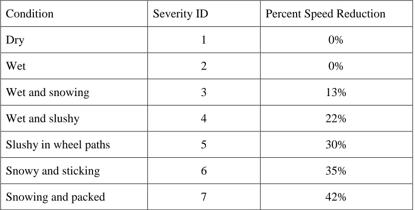
and weather data from 2002 to 2004. The FHWA (2010) classify weather conditions into
seven categories of road surfaces. Each road surface is designated with a severity IDs, and
was related to speed reductions. The FHWA categories were summarized in Table 2-2.
Table 2- 2. Speed reduction based on road surfaces. (Source: FHWA, 1977)
Condition Severity ID Percent Speed Reduction
Dry 1 0%
Wet 2 0%
Wet and snowing 3 13%
Wet and slushy 4 22%
Slushy in wheel paths 5 30%
Snowy and sticking 6 35%
Snowing and packed 7 42%
Due to the limitation of data and the interference of high rate of accidents occurred
during adverse weather conditions few studies were able to quantify the weather impact on
the traffic speed variation. Nevertheless, Stern et al. (2003) used a two-step linear
regression analysis to study weather condition such as precipitation types, wind, visibility
and pavement conditions on travel time. Result indicates an average of 14% increase in
travel time under adverse weather condition. Smith et al., (2004) provided two evident
explanations for this result are the surface friction and the presence of precipitation.
2.1.2 EFFECT OF WEATHER ON TRAFFIC VOLUME
Hanbali et al (1992) studied the reduction in traffic volumes during snowstorms in
rural areas of Illinois, Minnesota, New York, and Wisconsin. The result is summarized in
discretionary type of trips such as home to work and work to home. This study was
confirmed by Knapp (2000) indicating traffic volume reduces 16-47% in winter storm
events. Knapp included in his study factors such as: precipitation, air temperature below
freezing, wet pavement surface, wind speed and pavement temperature below freezing.
The data analyzed more than 4 hours in adverse weather and snowfall exceeds 5.1 mm/hr.
From the regression analysis, the study concluded that the percent volume reduction had a
significant relationship with total snowfall and wind speed. Capacity studies by Ries
(2004) on highway I-35W in Minneapolis and its suburbs indicates trace of rain reduces
volume of vehicles by 8%, each additional 0.01 inch of rain decreased capacity by 0.6%.
Similarly, the study by Hall and Barrow (1988) on the Queen Elizabeth Way in Hamilton,
Ontario concluded capacity is reduced because during rainstorms, traffic flow changes
from uncongested to congest at lower occupancy rates.
Table 2- 3. Volumereduction due to snowstorm. (Source: Hanbali and Kuemmel, 1992)
Precipitation Rate Weekdays Weekends
< 25 mm 7-17% 19-31%
25-75 mm 11-25% 30-41%
75-150 mm 18-34% 39-47%
2.1.3 EFFECT OF WEATHER ON EMISSIONS FROM TRAFFIC
In general the emission from traffic is affected by traffic speed and volume. The
emissions of vehicles on the road is related to the fuel usage based on the speed travelled
(FHWA, 2001). Research indicates the fuel usage is maximized at speeds between 50 and
90 km/h (Transportation Alberta (TA), 2000). At higher speeds the increased in
aerodynamic forces reduce fuel usage causing less air emissions. For highways, it is often
observed that the average speeds are often above the posted speed limit (TA, 2000).
However at congestion periods and bad weather conditions the reduction in speed can be
tremendous. At low speeds additional fuel is required to keep the engine running for the
same distance of travel, thus higher emissions is emitted (TA, 2000). In addition, trucks
vehicle on the road the greater the impact on air quality (Keuken et al. 2009). Figure 2-1
shows the speed in relation to emission of NOx and CO.
Figure 2- 1. NOx and CO emission produced from traffic in different speed. (Source:
FHWA, 2011)
Figure 2- 2. NOx emission from traffic in different speed and vehicle composition
(Source: The Department of Transport, England, U.K, 2005)
vehicles driven in adverse weather, a reduction in speed and volume was observed
(Alhassan, 2011, Maze, 2005). This affect is due to driver’s natural caution response
during bad weather (Lockwood, 2006). The changes in vehicular count and speed
reduction on roadway affect the total emission release into the environment. Logically,
reduction in traffic volume due to weather would decreases total emission. However,
increase in idleness would cause higher fuel consumption thus increase the emission.
Figure 2-3 shows the difference in emissions with higher NOx and CO concentrations
emits from cars than trucks.
Figure 2- 3. VOC, NOx and CO emission for car and trucks. (Source: FHWA, 2011)
From Figure 2-3, it can be seen that over the years, the total emission emits reduces
significantly due to high government restriction. Based on the review of traffic speed and
pollutants in the environment.
2.2 DISPERSION OF AIR POLLUTANTS FROM TRAFFIC
Dispersion of air pollutants is effected by meteorological conditions including
wind speed and wind directions. Due to the requirement of quantitating air pollution for
highway planning and roadway projects in early 1960 (Beychok, 2005), the atmospheric
dispersion models were developed. These models vary in methodologies including:
Gaussian plume models, puff models, box models, statistical modeling, and computational
fluid dynamics (CFD), geographical information systems (GIS), and wind tunnel
simulations. An extensive review of 30 dispersion models can be found in Holmes and
Morawska (2006). The most preferred types of dispersion model are those based on
proven Gaussian dispersion methodology for simulating air pollutant emissions from
industrial sources (IDNR, 2004). One applicable research for this methodology is by
Keuken et al (2009). In this study, HEAVEN software was used to modeled NOx and
PM10. This software is an approved line-source model in the Netherlands for assessing air
quality impacts of motorways under the environmental legislation (RIVM, 2008). Keuken
et al (2009) indicates speed reduction on the motorway reduces NOx by 5-30% and PM10
by 2-25%. Eneroth et al (2008) uses Airviro which is an approved program in Sweden. In
North America, a Gaussian-based highway models known as CALINE4 dispersion
modeling in an urban environment was assessed by Kenty et al (2006). This study also
modeled the pollutant of NO2 and NOx near Gandy Boulevard in Tampa, FL. Result
indicates CALINE4 under-estimate the chemical reaction NOx when ambient O3
concentrations is less than 40 ppb. Another complex model known as TAPM
accommodates both complex meteorology, topography and includes atmospheric
chemistry reaction. While this model provides high advantage, it also requires high
computer resources and long computation time (Wallace, 2008).
Statistical modeling of air pollution can be assessed by developing a relationship
between parameters such as meteorological and pollutant concentration estimates.
Techniques include regression, time series analysis Markov chain-Monte Carlo methods,
There are two types of CFD techniques: the diagnostic and prognostic. The
diagnostic interpolation methods are based on measurements that are subject to physical
constraints (Li et al., 2006). The prognostic uses three approaches the Reynolds-averaged
Navier-Stokes theory, the direct numerical simulation, and the large eddy simulation. This
type of dispersion model allows more detailed examination of vehicle-induced turbulence
in areas with complex street canyon geometries (Pierce, 2004), (Huber, 2006) uses CFD to
study human exposure factors and human exposure profiles dominated by local source
emissions.
Another method of modeling dispersion pattern resulting from vehicular emissions
is to use a GIS to map traffic related pollution. This method requires integration from other
models to calculate the impacts resulting from vehicular emissions. For example, Jin and
Fu (2004) study the application of GIS on modification of emission dispersion. This study
compared the observed hourly concentration and the simulated concentration. The
simulation concentration was derived from GIS and input into the Gaussian model which
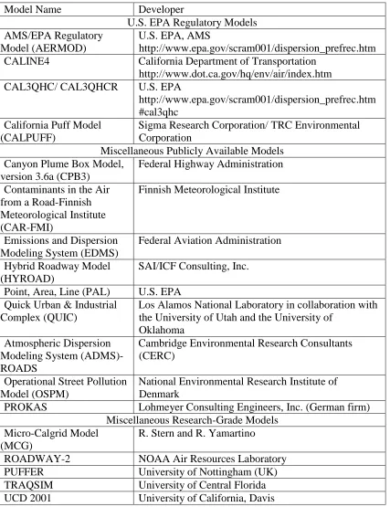
provides adequate results. Table 2-4 summarized the dispersion models reviewed by
Table 2- 4. Summary of Dispersion Models (Source: Table from Peirce et al, 2004)
Model Name Developer
U.S. EPA Regulatory Models AMS/EPA Regulatory
Model (AERMOD)
U.S. EPA, AMS
http://www.epa.gov/scram001/dispersion_prefrec.htm CALINE4 California Department of Transportation
http://www.dot.ca.gov/hq/env/air/index.htm CAL3QHC/ CAL3QHCR U.S. EPA
http://www.epa.gov/scram001/dispersion_prefrec.htm #cal3qhc
California Puff Model (CALPUFF)
Sigma Research Corporation/ TRC Environmental Corporation
Miscellaneous Publicly Available Models Canyon Plume Box Model,
version 3.6a (CPB3)
Federal Highway Administration
Contaminants in the Air from a Road-Finnish Meteorological Institute (CAR-FMI)
Finnish Meteorological Institute
Emissions and Dispersion Modeling System (EDMS)
Federal Aviation Administration
Hybrid Roadway Model (HYROAD)
SAI/ICF Consulting, Inc.
Point, Area, Line (PAL) U.S. EPA Quick Urban & Industrial
Complex (QUIC)
Los Alamos National Laboratory in collaboration with the University of Utah and the University of
Oklahoma Atmospheric Dispersion
Modeling System (ADMS)- ROADS
Cambridge Environmental Research Consultants (CERC)
Operational Street Pollution Model (OSPM)
National Environmental Research Institute of Denmark
PROKAS Lohmeyer Consulting Engineers, Inc. (German firm) Miscellaneous Research-Grade Models
Micro-Calgrid Model (MCG)
R. Stern and R. Yamartino
ROADWAY-2 NOAA Air Resources Laboratory
PUFFER University of Nottingham (UK)
TRAQSIM University of Central Florida UCD 2001 University of California, Davis
Among these models, the highly recommended model (EPA, 2005), for
(EPA, 2005). This model was used by Zou et. al. (2010) to study one, three and eight
hours period with daily, monthly, and annual SO2 concentrations. Zou et al (2010) found
that AERMOD performs better in simulating SO2 concentrations when combined both
point and mobile emission sources were inputs into the model rather than using point or
mobile emission sources alone. In addition, Kesarkar et. al. (2006) uses AERMOD to
study the impact of PM10 over Pune, India. This study suggested that AERMOD tends to
underestimates the pollutant concentrations especially over the city compared to rural. It is
believe to be attributed to the lack of background concentration in the model or the
under-representation of source profiles in the emission. A conference paper published by Kuwait
University (Saquer, 2007) examined SO2, non-methane hydrocarbon and NOx using
AERMOD. This study concluded there is a high degree of agreement 86%-98% between
predicted and measured concentration at different receptor locations.
2.3 SUMMARY
Based on this literature review, there are some limitations of previous studies.
Many studies have observed that adverse weather conditions such as poor lighting
condition, poor visibility and wet road condition reduce traffic speed and volume.
However, the reduced speed and volume are not only caused by adverse weather but also
by incidents or recurrent congestion. Thus, to analyze the effect of weather on traffic, the
relationship between weather on reduced speed and traffic volume should be identified.
Also, there is a lack of studies on the traffic emissions caused by adverse weather
condition. Thus, modelling the dispersion pattern of a NOx from traffic and examine the
concentration scatters over a distance in different weather condition should be addressed.
CHAPTER III
DESCRIPTION OF DATA AND STUDY SITE
3.1 STUDY SITE AND DATASETS
This thesis was focused on a section of the Gardiner Expressway in Toronto,
Ontario, Canada. The Gardiner Expressway is an urban freeway, frequently used by local
commuters going to and from downtown Toronto. The highway is presented in Figure
3-1,the Gardiner Expressway stretches 21.6 km long starting at Highway 427 at point A
extending to Don Valley Parkway at point B. The freeway generally spans 10 m wide in
each direction with the posted speed limit of 90 km/hr. The Gardiner Expressway resides
next to Lake Ontario (point E in Figure 3-1). At Highway 427 (point A), it is 2.9 km away
from the nearest point on the lake, where as at point B, it is 200 m away from the nearest
point on the lake.
Figure 3- 1. Map of Gardiner Expressway, Toronto, ON. (Source: Base map by Google,
2011)
There are two sets of data collected for this study. One set of data was for traffic
analysis and the other is for dispersion modeling. The first dataset for traffic analysis was
weekday hourly traffic record, and the incident logs. The second dataset are the weather
related data which were obtained from the Ministry of Environment Weather Office (MOE – WO) database website (2010). This dataset contains 3 files namely: the meteorology
data, the hourly weather observations and the hourly weather conditions.
3.2 TRAFFIC DATA
The traffic data collected were for the Gardiner Expressway in Toronto. This
freeway is a six lane highway with three lanes in each direction ran from east to west. At
any given time in the weekday, this highway contains approximately 2500 to 3000 cars per
hour, which equates to 67, 000 cars in the 24 hours period (CoT, 2010). Thus, making this
is one of the busiest highways in Toronto.
Along the Gardiner Expressway there are many detectors. The map file obtained
from the CTOOC shows 19 stations in each direction. The schematic drawing of this
section of freeway is shown in Figure 3-2. The traffic data was collected at station #80
highlighted in Figure 3-2, which is located near Kipling Ave on the both side of the
Arrow pointing outward = off-ramps, arrows pointing inward = on-ramps; letters inside squares = detector station IDs; number above or below station IDs = number of lanes; numbers between two successive detectors = distance (m); shaded detector stations = where traffic influenced by merging or diverging vehicles; bold number above or below distance numbers = total number of crashes in 13 months.
Figure 3- 2. Traffic stations along Gardiner Expressway. (Source: Lee et al., 2002)
3.2.1 WEEKDAY TRAFFIC
The Weekday Traffic files contain the occupancy, hourly speed and volume on the
road. The speed reading and the volume of vehicles on the Gardiner Expressway pertains
to the 24-hour period from zero to 23 hour. There are 193 days of records data for
eastbound and westbound direction. A sample of the raw data obtained at the loop
detector station 80 (highlighted in Figure 3-2) for the westbound direction is shown in
Table 3- 1. Raw data of speed and traffic volume on January 2nd, 1998. (Source: Toronto
Traffic Operation Office Center, 2010)
Time Speed (km/hr) Volume (veh/hr) Occupancy (%)
10:01:23 87 2340 1
11:01:23 91 1800 3
12:01:23 94 1980 4
13:01:23 97 2160 1
14:01:23 99 2160 2
15:01.23 86 2340 2
16:01:23 79 1980 3
17:01:23 89 1980 4
18:01:23 93 1980 1
In addition, the percentage of car and truck was provided by the City of Toronto
for the year 2001, 2004 and 2006. The averages of these three years indicated 90% of
passenger cars and 10% of trucks on this highway for both eastbound and westbound.
These percentages were used in the calculation of NOx emission in the later chapter.
3.2.2 INCIDENT LOGS
Detail record of incidents that occurred in 1998 was obtained from the incident
logs. Each incident was detected and verified by an operation at the control center and the
following information is recorded: a unique ID, date (year, month, and day), day of week,
station (closest upstream station to the incident site), the reported time, the type of
incidents (e.g. crash, construction), the weather condition and whether the incident was
Figure 3- 3. Sample of incident log for December 2, 1998. (Source: Toronto Traffic
Operation Office Center10)
3.3 WEATHER DATA
The weather data were obtained at the Center Island location (point C in Figure
3-1) which is 675 meter away from detector location station #40 (Figure 3-2). These data
were recorded according to the Eastern Standard Time (EST) in Toronto, Ontario. To
adjust for the daylight saving time (DST) months, a shift of one hour was added to all time
recorded.
3.3.1 HOURLY WEATHER CONDITIONS FOR TRAFFIC ANALYSIS
Weather data for the freeway were also obtained from the Weather Office. There
weather classification. The hourly weather observation was monitored for the total of 193
weekdays. Analysis shows in the 12-month period, 72.5 % of the 193 days was considered
to be adverse weather condition (of more than one hour of rain or snow). In the hourly
weather-observations, the conditions were labelled as either snow, rain, light rain or
drizzle. Forty-three hours are light rain, seven hours are drizzles, 278 are rainy, and 71
hours are snowy condition. The remaining hours are clear weather condition. Due to the
small number of light rain and drizzles, these were considered as rain and were combined
with other rainy condition. Table 3-2 shows the example of the data for January 8 -
January 10.
Table 3- 2. Example of weather condition. (Source: Toronto Traffic Operation Office
Center , 2010)
R- rain S: Snow L: light rain
Date 1 2 3 4 5 6 7 8 9 10 11 12 13 14 15 16 17 18 19 20 21 22 23 24
8-Jan R R R R R R R L L L
9-Jan S R R S S
10-Jan
S S S S S S S S S
The original hourly weather categorization, also taken from the Weather Office has
two files in excel format. One file listed the hourly records of temperature, dew point,
relative humidity, wind direction, wind speed, visibility and standard pressure. In this
study, visibility was extracted to use for analysis. The second file listed the daily
precipitation intensity among other variables which were extracted to calculate the hourly
precipitation concentration to use for analysis.
3.3.2 METEOROLOGICAL DATA USED FOR DISPERSION MODELING
The meteorological data were obtained from the MOE consists of two files: surface
scalar parameters, and the vertical profiles. Since no upper air surfaces data were collected
N, 78.73 o W), the nearest upper air station. The meteorology data was collected twice
daily at 7 a.m. and 7 p.m., Eastern Standard Time. The condition is assumed to be
consistent within a 500 km2 area zone (NOAA, 2010). Surface data were obtained at
Toronto City Airport (43.67oN, 79.60 oW) shown at point D in Figure 3-1. Interpolation of
the upper air condition in between the times collected was done using the meteorology
pre-processor, taking into consideration the local land use around Toronto. This process
was completed by the MOE and the data were downloaded from the website (MOE, 2010).
The example of pre-processed upper air data and surface is shown in Table 3-3 and Table
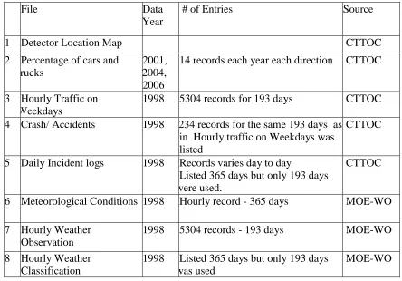
3-4, respectively. The listed of all the data collected and the number of records in each are
outlined in Table 3-5. The processing and use of these data will be presented in later
chapters.
Table 3- 3. Sample pre-processed upper air file. (Source: MoE, 2010)
Year Month Day Julian Day Hour
Sensitive Heat Flux (W/m2) Surface friction velocity (m/s) Convection velocity scale (m/s) * Year
98 1 1 1 1 -4.2 0.087 -999 98
98 1 1 1 2 -9.3 0.13 -999 98
98 1 1 1 3 -22.3 0.309 -999 98
Vert potential temp gradient above PBL* Height of convectively- generated boundary layer * Height of mechanically- generated boundary layer Morning Obukhov length (m) Surface roughness length (m) Bowen
ratio Albedo
Wind speed (m/s)
-999 -999 59 14.2 1 1.5 1 1
-999 -999 108 21.4 1 1.5 1 1.5
-999 -999 394 119.3 1 1.5 1 2.1
Wind direction (degrees)
Ref height for Ws & Wd (m)
Temp (K) Ref height for temp (m)
Precipitation code
Precipitation
(mm) * Humidity **
Pressure (Pa)
201 10 259.9 2 0 -999 9999 1013
258 10 262 2 0 -999 9999 1013
224 10 263.1 2 0 -999 9999 1013
* −999 for missing data.
Table 3- 4. Sample pre-processed surface file. (Source: EC, 2010)
Year Month Day Hour
Measurem ent height (m) Top flag Wind direction (degree) Wind speed (m/s) Temp (Kelvin) Standard dev of wind direction -F2 (degree)* * Standard dev of vertical wind speed -Fw (m/s)**
98 1 1 1 10 1 201 1 -13.3 9999 9999
98 1 1 2 10 1 258 1.5 -11.1 9999 9999
98 1 1 3 10 1 224 2.1 -10 9999 9999
** 9999 for invalid data.
Table 3- 5. Summary of data obtained from all sources
File Data
Year
# of Entries Source
1 Detector Location Map CTTOC
2 Percentage of cars and trucks
2001, 2004, 2006
14 records each year each direction CTTOC
3 Hourly Traffic on Weekdays
1998 5304 records for 193 days CTTOC
4 Crash/ Accidents 1998 234 records for the same 193 days as in Hourly traffic on Weekdays was listed
CTTOC
5 Daily Incident logs 1998 Records varies day to day
Listed 365 days but only 193 days were used.
CTTOC
6 Meteorological Conditions 1998 Hourly record - 365 days MOE-WO
7 Hourly Weather Observation
1998 5304 records - 193 days MOE-WO
8 Hourly Weather Classification
1998 Listed 365 days but only 193 days was used
CHAPTER IV
METHODOLOGY - TRAFFIC ANALYSIS
In this study, the speed variation is defined as the difference in speed between
normal weather condition and adverse weather condition. It is expected that the speed will
be changed due to adverse weather. However, speed will also be affected by traffic events
such as recurrent congestion and non-recurrent incidents. To isolate the effect of weather
on speed, the reduction in speed during recurrent congestion should be considered, and the
speed data collected when non-recurrent incidents occurred should be excluded. This
chapter outlines the deduction process and general overview of the data analysis.
4.1 NORMAL SPEED PROFILES
The normal speed profile (NSP) is defined as the average hourly speed when the
speed was unaffected by weather events and non-recurrent incidents. In other words, the
NSP represent the traffic flow on this freeway free from all incidents and weather
conditions and by no means indicate the traffic condition under uncongested or free-flow
traffic conditions.The incidents were obtained through incident logs at the City of
Toronto's traffic management center. Since the Normal Speed Profile includes average
hourly speed for each hour, each incident was assumed to effect speed for a maximum of
one hour period. If an incident occurred before 45th minute of the given hourly period, the
incident affects the speed in that given hourly period. If an incident occurred after 45th
minute of the given hourly period, the incident affects the speed in the next hourly period.
For example, if the incident occurred at 5:15 p.m., then it affects the speed from 5 -6 p.m.
However, if the incident occurred at 5:47 p.m., then it affects the speed from 6 – 7 p.m. If
these two incidents occurred then the duration is 2 hours in total.
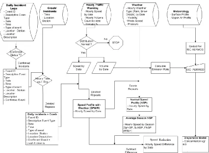
The processes to generate the Normal Speed Profile are as follow. First, false alarm
incidents were filtered from the data. Speed data affected by the real incidents were
removed. The remaining speed data are the speed affected by weather only.
Visual Basic coding for these elimination processes are in Appendix A. The 193 days in
Hourly Traffic data yields 5204 hours for analysis. All missing speeds or volume were
replaced with a star, during analysis.
Figure 4- 1. Process flowchart of all data
4.2 PRECIPITATION AND VISIBILITY
The weather data collected from the Weather Office contained one daily total
precipitation intensity (mm) file and one hourly visibility and weather classification file.
Visibility was measured in the unit of distance and the value ranges from 0 to 15 km. High
visibility indicates good weather conditions. In a clear day the visibility ranges from 10-15
km (Weather Network, 2011).
Since only daily precipitation intensity was provided, this was used to estimate the
each weather classification lasted for one hour. For example, if the weather is classified as
rainy condition at 5 p.m., then it was assumed that it rained from 5 -6 p.m. The hourly
precipitation rate is the total daily precipitation divided by the number of hours with rain,
snow or drizzle weather condition on that day. For example, with the weather conditions
record for January 9th in Table 3-2, there were five hours and daily precipitation of 4.5
mm, the hourly precipitation is 0.9 mm/hr. This hourly precipitation rate is consistent for
the 3 hours of snow and 2 hours of rain in January 9th, 1998.
4.3 DAYLIGHT CONDITION
Since there was a difference in time stamp between Daylight Saving Time and
Eastern Standard Time in the Northern Hemisphere, the lighting conditions were
categorized separately for these time periods. Eastern Standard Time starts from the first
week of November and ends in mid-March. In these months, the daytime is from 8:00
a.m to 6:59 p.m and the nighttime is 7:00 p.m to 7:59 a.m. The Daylight Saving Time
starts from mid-March and ends in the first week of November. During these months, the
daytime is from 7:00 a.m to 7:59 p.m and the nighttime is 8:00 p.m to 6:59 a.m.
4.4 SPEED REDUCTION
To better understand how weather condition reduces speed without being affected
reduction from recurrent congestion, speed reduction was used for analysis. Speed
reduction is defined as Normal Speed Profile minus actual hourly speed excluding
non-recurrent events such as accidents and incidents. The positive values indicate speed
reduction, whereas negative values indicate higher speed than speed under the normal
condition. Speed reduction was categorized into 4 subsections for analysis: no speed
reduction, >5 km/hr, 5-10 km/hr and > 10 km/hr. The difference between Normal Speed
profile and the observed speed without non-recurrent incidents would exempt any effect
due to recurrent congestion such as rush hour. An example of speed variation for April
30th is shown in Figure 4-2. The difference in speed reduction due to non-recurrent
incidents.
.
Figure 4- 2. Hourly variation in speed reduction on April 30, 1998
Due to the nature of the data the speed reduction was used as a categorical variable
because there as insufficient data to use as a continuous variable. If continuous variable
was used there will be very small number of samples for a specific speed reduction and it
limits the advantage of observing the general relationships between speed reduction and
weather related factors.
4.5 STATISTICAL METHODS
The Statistical Analysis System (SAS) (2008) format is used for statistical testing.
SAS is an integrated system of software products provided by SAS Institute Inc, which
enables users to perform computational statistical analysis. A SAS program has three
major parts: the data, categorization steps procedure (if required), and the macro
programming language that direct the software to conduct the analysis. At runtime, the
data are compiled and the software run the sequence procedures based on the interpreted
macro coding as they appear in the SAS program.
investigate the effect of weather on speed reduction. They are the Chi-square test and the
Logistic Model known as Ordered Logistic Regression.
4.5.1 CHI-SQUARE TEST
Chi-square is a statistical test commonly used to compare observed data with the
expected data obtained in reference to the null hypothesis. The null hypothesis states that
there is no significant difference between the expected and observed result. In other words,
the null hypothesis is that there is no relationship between the two factors being
considered. The alternative hypothesis is that there is a relationship between the two
factors being considered. The null hypothesis will be rejected when the test statistic has a
p-value ≤ 0.05. The Chi-square is the sum of the squared difference between observed (O)
and the expected (E) value (or the deviation, d), divided by the expected data in all
possible categories. This can be express as:
E E O X
2
2
( )(1)
where: O = observed data
E = expected value
X2 = chi square value
The higher the Chi-square values the stronger the relationship between the
variables. The probability value is calculated alongside with the Chi-square test. In
addition there is another “parameters estimate” can express the likelihood relationship of
the data sample such as the p-value. The probability value or p-value is such a parameter.
If the p-value is less than 10%, this means the relationship between the variables has a
90% confidence. From this statistical test, the Chi-square value and the p-value will
indicate how strong the weather variables in relation to the speed observed.
4.5.2 LOGISTIC REGRESSION: ORDERED REGRESSION MODEL
k kx b x b x b a i Y P i Y P
Ln ] ...
) ( 1
) (
[ 1 1 2 2
( 2 )
where,
P(Y = i) = the probability that Y belongs to category i;
a = a constant;
bk = a coefficient for the kth explanatory variable;
Xk = explanatory variable.
Logistic regression does not assume a linear relationship between the dependent
and independent variable. The relationship between the dependent and independent
variable may be linear or nonlinear. Also it does not require the sample to be normally
distributed. In fact the sample can be normal, Poisson or Negative Binominal. In addition,
this model does not assume that there is an equal variance among all independent
variables.
There are some limitations of this model as follows. The dependent variable in the
data sample should be dichotomous in nature. The error term is assumed to be independent
for each variable. Although logistic regression does not assume a linear relationship, the
relationship between the odds ratio and the independent variable is linear. However, since
the weather data are categorical in nature, this model is more suitable for investigating the
effect of weather on speed reduction.
The logistic regression does not account for the ordinal nature of the categorical
variables. Subsequentially, a subset of this model known as the Ordered Logistic Model
was considered. This model was chosen because the categories of speed reduction within
our data are ordinal in nature. In other words, a model was selected to compare the
difference between higher level and low level magnitude of effects. In ordered regression,
the dependent variable is ranked (Logistic regression, 2010). The first category is usually
considered as the lowest category (first ordered) and the last category is considered as the
highest category (last ordered) (Gelman, 2007) or vice versa. In other words, the higher
level represents higher magnitude of effects than lower levels. The ordered model is
described as follows (Kleinbaum, et al., 2008).
i k k 2 2 1 1 *
i b x b x ... b x ξ
Y (3)
Yi* = the independent variable which is an indicator of category of speed reduction
b = coefficient
xk is the independent variable including visibility, precipitation, season, weather
condition, lighting condition
i
ξ is the random error term
The category of the dependent variable (speed reduction) is predicted based on Yi*
based on the following criteria:
Yi = 1 if Yi* <= 1
Yi = 2 if 1 < Yi* <= 2
: : :
Yi = m if Yi* > m-1
where m = number of categories for that dependent variable
1, 2....m = the threshold values of each category in Table 4-1.
4.6 VARIABLE CLASSIFICATIONS
Before examining the relationship between speed and speed reduction with weather
variables, the variables must be categorized. The classifications of each parameter are
shown in Table 4-1.
Table 4- 1. Classifications of Variable for analysis
Variables # cat Classifications
Speed (km/hr) 5 Congested : <60, 60 -80
Free flow : 80-90 90-100 >100 Speed reduction
(km/hr)
4 No reduction; > 0 and 5 > 5 and 10 > 10
Precipitation (mm/hr)
3 0 0.05-5 >5
Visibility (km) 3 0-5 (low) 5-10 (med) 10-15 (high)
Season 4 Spring Summer Fall Winter Weather 3 Clear Rain Snow
CHAPTER V
RESULTS OF TRAFFIC ANALYSIS
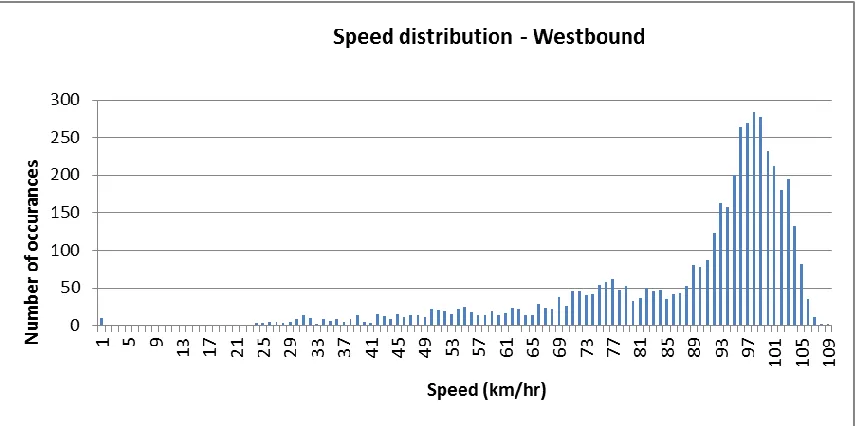
5.1 SPEED DISTRIBUTION
To better understand the trend of the data collected, the distribution of all hourly
speeds was graphed. Figure 5-1 and 5-2 shows the histogram of speed distribution for the
193 days for westbound and eastbound direction.
Figure 5- 2. Eastbound speed distribution for 1998
The westbound speed ranges from 0 – 108 km/hr, whereas it is 0- 99km/hr for
eastbound. The average lies at 86.7 km/hr for westbound and 81.6 km.hr for eastbound.
Speed over 80 km/hr was considered as the speed free of congestion. For further analysis
of weather on speed, the free-flow speed was categorized into 3 subsections: 80 – 90
km/hr, 90-100 km/hr and above 100 km/hr. The congested speed was categorized into 2
subsections: 0-60 km/hr and 60-80 km/hr. These categorizations were based on the
different emission trend for each speed in Figure 2-2.
5.2 VOLUME DISTRIBUTION
The volume distribution for Gardiner Expressway in 5304 hours is shown in
Figures 5-3 and 5-4. In westbound lane the volume ranges from 0 – 2164 veh/hr with the
average of 1221 ve/hr. In eastbound lane the volume ranges from 0- 2151 veh/hr with the
Figure 5- 3. Westbound volume distribution for 1998
Figure 5- 4. Eastbound volume distribution for 1998
To calculate the emission of NOx, a closer look at between the clear weather
condition and adverse weather condition was examined. The volume distribution between
399 hours of adverse weather and 399 hours of clear condition is shown in Figures 5- 5 –
5-8. The clear hours are selected based on the hour subsequent ot the day that either rain or
of same hour did not meet the visibility condition then the following day was condisered.
All volume were above zero vehicle per hours. The minimal traffic volume use for
eastbound is 71 veh/hr for clear and 86 veh/hr for adverse weather condition. In
westbound direction the minimum traffic volume used is 226 veh/hr for clear and 246
veh/hr for adverse weather condition.
Figure 5- 5. Westbound volume distribution for 399 hours of clear weather condition
Figure 5- 7. Eastbound volume distribution for 399 hours of clear weather condition
Figure 5- 8. Eastbound volume distribution for 399 hours of clear weather condition
5.3 MONTHLY NORMAL SPEED PROFILES
To compare the difference in the Normal Speed Profile among four seasons, the
monthly and seasonal patterns of Normal Speed Profile for east and westbound were
month. The total number of incidents for both directions is shown in Table 5-1. The
westbound lane monthly Normal Speed Profiles are shown in Figure 5-9 - 5-12 based on
the seasons. For the corresponding months on each season please refer to Table 4-1. Noted
that December of 1998 occurred at the end of the year was combined with January and
February at the beginning of the year to mark the winter season. Monthly NSP was used
for to minimize the deviation of the speed profile in each season.
In traffic research, it is common that traffic flow conditions are different based on
the hour of the day. The trends for this highway can be observed in Figures 5-9 – 5-12. In
the westbound lane, speed slows during morning peak of 7 a.m. to 10 a.m., two off peak
periods are 11 am to 3 pm and 9 pm to 7 a.m., and an afternoon peak period at 3 pm to 9
pm. In the afternoon peak periods, speed significantly dropped more than the morning
peak period. The afternoon peak went well below the free-flow speed of 100 km/hr. The
speed variation shown in Figure 5-13 indication most speed varies within 25 km/hr range
of the average speed.
Table 5- 1. Number of total non-recurrent incidents by season
Westbound Eastbound
Spring 379 130
Summer 711 223
Fall 487 111
Winter 430 112
Figure 5- 10. Spring Normal Speed Profile in westbound direction.
Figure 5- 12. Fall Normal Speed Profile in westbound direction.
The eastbound lanes Normal Speed Profile is shown in Figures 5-14 – 5-17. Here
morning peak is at 7 a.m. to 11 a.m., and off morning peak from 1a.m – 6 am and an
afternoon peak period at 4 pm to 9 pm. In the morning peak period, there is a slight
reduction in speed. However, in the afternoon peak periods, speed significantly drops
below free-flow speed of 100 km/hr. The speed observed for eastbound lane ranges from
zero km/hr to 99 km/hr. Figure 5-18 show the speed variations are within 25 km/hr limit
with higher variation occurred in the afternoon than in the morning period.
Figure 5- 15. Spring Normal Speed Profile in eastbound direction.
Figure 5- 17. Fall Normal Speed Profile in eastbound direction.
Figure 5- 18. Variations in speed profiles for eastbound direction.
Due to different peaks periods between westbound and eastbound, speed reduction
characteristic to this freeway. The reason for this is due the ramp closure in the afternoon
specifically from 3 p.m – 6 p.m. This ramp reopens at 6:00 p.m for both directions thus
causes longer and lower afternoon peak than morning
The usage of speed reduction, in turn, will eliminate factors between congestion
and un-congestion periods, whereby reflecting the delay of speed travelled.
5.4 RELATIONSHIP OF WEATHER AND SEASON WITH SPEED - RESULT OF
CHI-SQUARE TEST
To determine whether the relationship between the observed speed and weather
conditions was significant, the Chi-square test was performed. Lighting condition,
precipitation, visibility, season and weather condition were related to speed and their
association was assessed. The complete SAS output of all tests provided in Appendix C.
However, the graphical results of the relationship between speed and the factors in
Chi-square tests are shown below.
Figure 5-19 shows the relationship between speed and lighting condition. Based on
the graphs in Figure 5-19, it was found that higher speed is more likely to occur at
nighttime and lower speed occurs at daytime. This is due to less traffic volume on the road
at nighttime as seen in Figure 5-20. In eastbound direction, the medium flow speed of
60-80 km/hr and 60-80-90 km/hr is constant, whereas it was marginally higher in nighttime then
daytime in westbound. The association between speed reduction and lighting condition is
Figure 5- 19. Relationship between speed and lighting.Result of Chi-square test,
relationship is significant at p < 0.01
Figure 5- 20. Relationship between traffic volume and lighting condition.
Figure 5-21 shows the relationship between speed and precipitation. As seen, speed
is likely to be higher at low precipitation as shown in Figure 5-21 (a) and (b). One
free-flow speed westbound show a consistent distribution throughout all precipitation
rates. However, eastbound lanes provide a clear trend that the higher the precipitation rate
the lower the observed speed. As expected, at low precipitation drivers have more control
of the vehicle and the road surface friction is high. Again the correlation was significant at
a 90% confidence interval (p-value 0.10).
Figure 5- 21. Relationship between speed and precipitation. Result of Chi-square test,
relationship is significant at p < 0.1
Figure 5-22 shows the relationship between speed and visibility. The Chi-square
test shows a strong correlation between visibility and speed (p-value 0.10). In westbound
[Figure 5-22 (a)] high speed is likely to occur at both high and low visibility. However, in
eastbound [Figure 5-22 (b)] the lower speed is likely to occur at low visibility. Speed is
constant in medium speed ranges of 60-80 and 80- 90 km/hr in both westbound and
Figure 5- 22. Relationship between speed and visibility. Result of Chi-square test,
relationship is significant at p < 0.1
Figure 5-23 shows the relationship between speed and season. On both westbound
and eastbound directions, result indicates high speed is likely to occur in fall season than
any other seasons and low speed is likely to be lower in summer. This is because traffic
volume is lower in fall and high in summer when the outdoor activities are more frequent,
as can be seen in Figure 5-24.
Figure 5- 23. Relationship between speed and season. Result of Chi-square test,
Figure 5- 24. Relationship between volume and season for westbound and eastbound
direction.
Figure 5-25 shows the relationship between speed and weather classification. The
Chi-square test shows a marginal relationship (p-value 0.10). Speed is likely to be higher
in clear weather condition than adverse weather conditions. In adverse weather
conditions, speed is likely to be lower in snowy condition than rainy condition, especially
in eastbound direction. This may be due less surface friction on the road which cause
slippery in snowy condition leading driver to be cautious. In westbound direction medium
free-flow speed of 60-80 km/hr occurred in snowy condition, whereas it occurred in rainy
Figure 5- 25. Relationship between speed and weather conditions. Result of Chi-square
test, relationship is significant at p < 0.1
5.5 RELATIONSHIP OF WEATHER AND SEASON WITH SPEED REDUCTION-
RESULT OF CHI-SQUARE TEST
To eliminate the effect of congested and uncongested traffic on the highway, speed
reduction between the Normal Speed Profile and the observed speed was calculated. The
speed reduction is positive when the observed speed is lower than Normal Speed Profile.
If the observed speed is higher than Normal Speed Profile, it is classify as no speed
reduction. The results of the Chi-square tests are examined below.
Figure 5-26 shows the relationship between speed reduction and lighting condition.
Speed reduction is likely to be higher at nighttime than daytime, especially in eastbound
direction. This is mainly because of the volume difference between daytime and nighttime.
Thus, the calculated average speed in Normal Speed Profile at daytime is lower than
average speed at nighttime. Therefore, the observed speed at daytime is likely to be higher