Development of Floor Design Response Spectra. Rules and Practice

Development of Floor Design Response Spectra. Rules and Practice.

Peter Vasilyev

CKTI-Vibroseism, Saint-Petersburg, Russia ABSTRACT

Most of NPP’s equipment and piping have to be designed to withstand the effects of earthquake. These components have to be verified by analysis or by experimental testing. Design Floor Response Spectra (FRS) usually represent an input seismic excitation for a floor supported equipment and piping. The development procedure for floor response spectra is described in a number of official documents. Among them is the US NRC Regulatory Guide 1.122 [1] recognized as the most comprehensive and competent one. Above-mentioned document (revision 1) is of February 1978.

Current practice for the development of floor design response spectra meets a number of problems and questions, which still have no answers in Standards and Guides used for Nuclear Industry. As a result, a structural engineer can make a decision, which can lead to essentially more or less conservative analysis without violation of the prescribed requirements.

The presented paper is dedicated to discussion of the questions and problems connected with development of floor design response spectra. The paper also proposes some directions to improve the existing Codes and Regulations. Some problems, discussed in the paper, are specified below.

The damping level in the structure and in the soil has an essential impact on the response accelerations. In practice there are two general methods for calculation of nodal acceleration response time histories. Both of them have the own specific features and weak points for accounting of damping phenomenon.

Also there are two questions regarding the frequency range of FRS: upper limit (cut-off frequency) and a number and values of frequencies in a set.

In practical calculations several variants of the soil properties, source seismic excitations and a number of the nodes should be considered for FRS generation. It means that Design Floor Response Spectra is a result of convolution procedure. From the other hand, there are several ways how to do it.

The requirement of the soil characteristics variation is in some contradiction with the spectrum peaks broadening procedure. The spectrum peaks broadening procedure is intended for the uncertainties compensation. However, these uncertainties include soil characteristics among the other.

The highlighted problems are illustrated by the numerical examples using the finite element models of the actual nuclear related buildings.

INTRODUCTION

Most of NPP’s equipment and piping have to be designed to withstand the effects of earthquake. These components have to be verified by analysis or by experimental testing. Floor Design Response Spectra usually represent an input seismic excitation for a floor supported equipment and piping. The development procedure for the floor response spectra is described in a number of Standards and Guides. Among them is the US NRC Regulatory Guide 1.122 [1] recognized as the most comprehensive and competent one. Above-mentioned document (revision 1) is of February 1978. Some requirements are in the more modern codes [2] – [5].

Current practice in developing of the floor design spectra and subsequent piping and equipment analyses has revealed some question and problems, which have no answers in rules and codes. The suggestions and decisions, engineer can make, might lead to conservative as well as non-conservative result without a violation of code requirement.

The development procedure for the floor response spectra can be divided to the next stages:

1. Seismological investigation on the site. Seismic events intensity definition should be done based on probabilistic procedure. Design Response Spectra should be developed on the free soil surface for the cases of OBE and SSE.

2. Development of the soil and building models. Soil Structure Interaction (SSI) problem is often investigated at this stage. As a result of this study Input Seismic Excitation for subsequent structural analysis can be re-evaluated and adjusted.

3. Calculation of the nodal acceleration time histories and corresponding response spectra. The ground properties and source excitation are usually varied during this analysis.

4. Resultant Design FRS generation.

Only several questions and problems that arise during practical floor spectra development are discussed below.

DAMPING

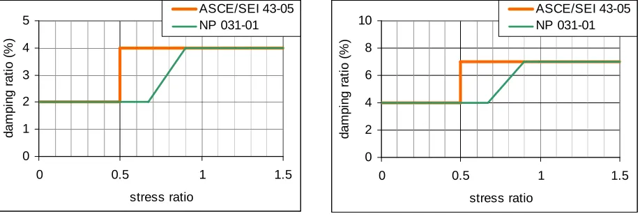
There are two modern codes, which contain requirements for the damping values used for floor response spectra development: American Code ASCE/SEI 43-05 [3] and Russian Code NP 031-01 [4]. Both documents specify damping values as a function of stress level in structure. Comparison of damping values for the two types of structures is shown in fig. 1 and fig. 2.

0 1 2 3 4 5

0 0.5 1 1.5

stress ratio d a m p in g r a ti o ( %) ASCE/SEI 43-05 NP 031-01 0 2 4 6 8 10

0 0.5 1 1.5

stress ratio d a m p in g r a ti o ( %) ASCE/SEI 43-05 NP 031-01

Fig. 1 Damping Values for welded metal structures Fig. 2 Damping Values for reinforced concrete structures

It is difficult however to implement this requirements in practice. Engineer has to proceed several iterations to recalculate stresses and adjust the damping value. Also, there is a lack of formal stress level calculation procedure for a whole structure. These difficulties lead to changing these requirements. It is often that low damping values are used for OBE and high damping values are used for SSE. It may be more rational to treat the damping values as a function of seismic excitation intensity (ZPGA).

In the practice there are two general methods to get nodal acceleration time histories. The first one is the Direct Time History Analysis. This method uses stiffness, mass and damping matrices directly to solve the system motion equations. The second one is the Modal Time History Analysis. This method consists of three stages: modal analysis, time history solution using modal coordinates and nodal acceleration calculation as a sum of modal accelerations.

Both of methods have their own features for damping modelling.

The first method allows taking into account the local damping and the local nonlinear behavior in general. This gives an opportunity to take into account the high damping in the ground by adding viscous elements to the model. From the other hand this method uses Rayleigh damping in the structural elements. Rayleigh damping is defined by two numbers and applied to the structure as a whole. This damping depends on oscillation frequency. The dependency can be expressed by the following equation:

)

2

2

(

2

1

1

_R

_f

f

R

d

π

π

+

⋅

⋅

=

where R1 and R2 are damping parameters, f is a frequency in Hz. Sample damping-frequency curve is shown in the fig. 3. The most conservative rule to choose Rayleigh numbers is to make damping curve lower than required damping in the frequency range between the first natural frequency of the structure (FL) and

cut-off frequency (FR). However this rule looks much

conservative. Probably the more rational rule will looks like the follow: damping curve d(freq) should be developed using two points: dL(FL) = 1.1*d and dR(FR) = 1.3*d, where d – required damping value.

The second method (Modal Time History Analysis) allows defining exact damping value for each mode. This provides possibility to follow code requirements. However this makes impossible taking into account damping in the soil. The last reason may lead to excessive conservatism. 0 0.01 0.02 0.03 0.04

0 2 4 6 8 10 12 14 16 18 20 22 24 26 28 30 32 34 36 38 40 frequency, Hz d a m p in g r a tio

FREQUENCY RANGE

Usually it is not difficult to choose the left limit of the frequency range – FL. It is important to define FL below the

first natural frequency of the piping or equipment, which will be subsequently analyzed using floor response spectra. Practically this value lies in a range from 0.1 to 0.5 Hz. It is not a good idea to set FL equal to zero. In this case it will be

impossible to use logarithmic interpolation for the spectrum values.

However, choosing of the right limit of the frequency range FRis more difficult task . This value has essential

influence on subsequent analysis accuracy. There are several possible approaches for defining FR value. Three of them

approaches are discussed below.

1) Definition by input seismic excitation response spectra.

This approach uses information about frequency range in the source seismic excitation. Right part of the response spectrum, with the acceleration values below some level (for example, ZPGA+10%), could be treated as not essential and could be cut off. Algorithm may be illustrated by fig. 4. If someone implements this procedure it will be necessary to define not only acceleration level, but also damping value for response spectrum. Usually we have a set of spectra for different directions and different possible earthquake sources. In this case we have to choose maximum value for the cut-off frequency (FR). This approach guarantees that essential components of a possible earthquake will not be neglected.

2) Definition by floor response spectra.

Comparison of Ground and Floor Response Spectra often leads to observation that some high frequency components have been filtered out. In this case FR value can be shifted to the left as

shown in the fig. 4.

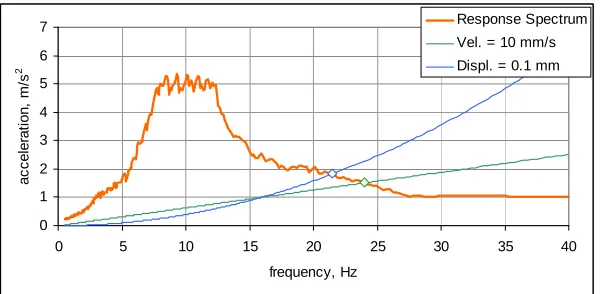
3) Definition by the “safe” velocity or displacement. If it is possible to define some “safe” values for the velocities or displacements in the seismic response, it would be possible to bound response spectra as shown in fig. 5. “Safe” value for velocities can be developed, for example, using vibration code. “Safe” value for displacements can be developed on the basis of fracture mechanics. This approach may be very useful for high frequency impacts such as airplane crash or blast wave analyses.

It should be noted that high FR

values may lead to non-conservative results in subsequent analyses. If some first natural frequencies of equipment lie in the “hard zone” of the FRS, equipment's modal responses will be close to ZPA. In this case SRSS method could produce results less than response obtained by the static method. This problem may be also eliminated using modern and more sophisticated summation methods.

Regulatory Guide [1], ASME BPVC [5] and NP [4] recommend minimal frequency set to develop floor response spectra (75 points). It also requires including in this set natural frequencies of the building. It is obvious that this requirement was developed at the age of stick-models. Modern models of building structures contain thousands degrees of freedom and hundreds natural frequencies in the range of interest. To meet this requirement in case of direct THA an additional analysis should be

0 5 10 15 20 25

0 5 10 15 20 25 30 35 40

frequency, Hz a cc e le ra ti on , m/s 2 ground floor ZPGA + 10% floor ZPA + 10% F-max = 26.9 Hz F-max = 22.5 Hz

Fig. 4 Sample source response spectrum and floor response spectrum. FR (F-max) value definition.

0 1 2 3 4 5 6 7

0 5 10 15 20 25 30 35 40

frequency, Hz a c c e le ra ti o n , m /s 2 Response Spectrum Vel. = 10 mm/s Displ. = 0.1 mm

Fig. 5 Response spectrum and the curves with constant velocity and constant displacement.

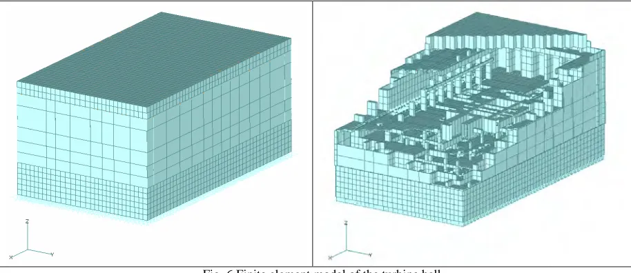
performed to calculate a set of building's natural frequencies. The actual model of the Turbine Building is presented in the fig. 6. Size of this model is not too big with respect to modern FE technologies. It contains 13393 nodes, 19763 elements and 62930 degrees of freedom. Results of modal analysis showed 770 natural frequencies in the range below 30 Hz.

Fig. 6 Finite element model of the turbine hall

It's evident that requirement to add all these frequencies to the frequency set looks much excessive. From the other hand the minimal frequency set does not look conservative enough, especially for the low damping values. Most attractive variant is to use a uniform set instead of this minimal set. The uniform set can be defined using the following recurrent expression:

)

1

(

1

F

d

F

=

⋅

+

α

⋅

where α - parameter, d – damping ratio.

The results of the numerical experiment are shown in the fig. 7 and fig. 8. A set of several accelerograms was used to compare maximum spectrum values and to estimate possible error. This "relative error" was defined as:

0

0

)

(

_

A

A

A

error

relative

=

−

where: A0 – is FRS maximal peak acceleration found in the whole frequency range for "accurate" FRS developed with dense frequency set. Ai – the same value for FRS developed using some values of d and α.

0 5 10 15 20 25 30 35 40

0 0.05 0.1 0.15 0.2 0.25

parameter alpha*d

re

la

tiv

e

e

rr

o

r

(%)

d = 1% d = 2% d = 5% d = 10% d = 20%

0.001 0.01 0.1 1 10 100

0.01 0.1 1 10 100

parameter alpha

re

la

ti

v

e

e

rr

o

r

(%)

d = 1% d = 2% d = 5% d = 10% d = 20%

Fig. 7 Relative error against parameter α*d Fig. 8 Relative error against parameter α

When parameter α is equal to 1.0 and relative damping is of 2% there will be 260 frequencies in the range from 0.2 Hz to 34 Hz. This number is greater than number of frequencies in the minimal recommended set (75 frequencies), but lower than number of natural frequencies of the building model (770 frequencies).

GENERALIZATION OF THE SPECTRUM

ASCE-4-98 [2] requires using of the three variants (not less) of the soil characteristics. Besides, there are usually several variants of the source (input) seismic excitation. And finally, the place where equipment or piping is attached to civil structure is modelled with several nodes of FE model. Thus we need to convolute many spectra into one generalized spectrum for each direction and each damping ratio. Spectra have to be convoluted for three parameters: computational nodes, different source excitations and varied soil characteristics. In addition to convolution, usual procedure includes spectrum smoothing and spectrum peaks broadening. There are several ways for such a convolution. Among them are:

- maximum value (enveloping); - mean value;

- median value plus one standard deviation.

Of course, other approaches may be used, but three operations mentioned above are most popular in the practice. The convolution order may be neglected in some trivial cases: for example, if convolution for all three parameters uses maximum value criterion. But in general, convolution order will affect the resulting spectrum.

Nodal convolution has to be done using maximum value. The only way of decreasing conservatism on this stage is specification of the exact place in the model where piping/equipment is located (less nodes should be processed).

Convolution for soil characteristic variants and convolution for different excitations can be done using other operations because these variants can be considered from probabilistic point of view.

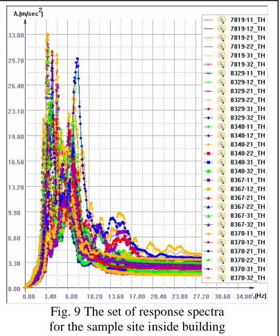
All mentioned above is illustrated by sample of FRS generation procedure. FE model of the turbine hall (fig. 6) is used in this sample. Two variants of source seismic excitation are applied to the model. Three variants of the soil characteristics are investigated. The site of the interest contains five nodes. Only one direction (Y) and one damping ratio (2%) are studied in this exercise. Thus 30 response acceleration TH are the input data set for the generalization procedure. The family of the 30 corresponding spectra is shown in the fig. 9.

Fig. 9 The set of response spectra for the sample site inside building

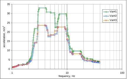
Three variants of the convolution procedure were investigated: Variant 1:

1) Convolution for nodes, soil characteristics and different excitations with use of enveloping (maximum value approach)

2) Spectrum peaks broadening by ±15%. Variant 2:

1) Convolution for nodes: enveloping;

2) Convolution for soil characteristics: mean value;

3) Convolution for excitation variants: “median plus one standard deviation”. 4) Spectrum peaks broadening by ±15%.

Variant 3:

1) Convolution for excitation: “median plus one standard deviation”. 2) Convolution for soil characteristics: mean value.

3) Convolution for nodes: enveloping 4) Spectrum peaks broadening by ±15%.

It's clear that the first variant is the most conservative and the order of the convolution's operation is not significant. The second and third variants differ from one another only by the order of convolution operations. The comparison of the resulting generalized floor response spectra is shown in the fig. 10.

0 5 10 15 20 25 30 35

1 10 100

frequency, Hz

a

c

c

e

le

ra

ti

o

n

,

m

/s

2

Var#1 Var#2 Var#3

Fig. 10 Resulting generalized floor response spectra

It is obvious that the fist variant is sufficiently more conservative than two others. The second variant and the third one differs a little, however ZPA value for the third variant is higher than for the second one by 16%.

SOIL PROPERTIES VARIATION AND PEAK BROADENING

For the same reason ASCE-4-98 [2] requires the use of three variants of the soil properties: “Low strain soil shear modulus shall be varied between the best estimate value times (1 + Cv) and the best estimate value divided by (1 + Cv), where Cv is a factor that accounts for uncertainties in the SSI analysis and soil properties.” Cv = 0.5 is the minimum value. When insufficient data are available to address uncertainties in soil properties, Cv = 1.

EUR [6], developed by the main European industry leaders, recommends common approach for any soil. It recommends making analyses for nine (!) tabulated variants of the soil properties plus one variant on the absolutely rigid base. This document recommends enveloping these ten spectra but not recommends spectra peaks broadening.

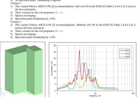
Mentioned above is illustrated by the next sample. Finite element model of the building is shown in fig.11. Sample procedure was applied to one node of the model, one spatial direction and one variant of the source seismic excitation.

Three variants of the generalization procedure are investigated: Variant 1:

1) This variant follows EUR [6] recommendations. Nine variants for the soil properties + one rigid base variant. 2) Spectra enveloping.

3) No spectrum peaks’ broadening is applied. Variant 2:

1) This variant follows ASCE-4-98 [2] recommendations. Soft soil (#2 in the EUR [6] Table 2.4.6.4.2.4) is used as the best estimation.

2) Three variants for the soil properties. Cv = 1. 3) Spectra enveloping.

4) Spectrum peaks broadening by ±15%. Variant 3:

1) This variant follows ASCE-4-98 [2] recommendations. Medium soil (#5 in the EUR [6] Table 2.4.6.4.2.4) is used as the best estimation.

2) Three variants for the soil properties. Cv = 1. 3) Spectra enveloping.

4) Spectrum peaks broadening by ±15%.

0 5 10 15 20 25 30 35

1 10 100

frequency, Hz

a

cc

e

le

ra

ti

on

,

m

/s

2

Var#1 Var#2 Var#3

Fig. 11 Sample concrete building model Fig. 12 Resulting generalized floor response spectra The comparison of the resulting generalized floor response spectra is shown in the fig. 12.

It is shown, that resulting spectrum is very sensitive to soil properties and their variations. The use of the spectrum in the first variant cannot be recommended because of subsequent analysis results will be too sensitive even to the small uncertainties in the model.

CONCLUSION

It will be rational to develop official recommendations or requirements in the borders of IAEA and ASME Codes or other relevant Standards for creating floor response spectra for both seismic and extreme dynamic load analysis.

REFERENCES

1. U.S. Nuclear Regulatory Commission (1978) Regulatory Guide 1.122 – Development of Floor Design Response Spectra for Seismic Design of Floor-Supported Equipment or Components. Revision 1, February 1978

2. ASCE-4-98, Seismic Analysis of Safety-Related Nuclear Structures and Commentary, 2000

3. ASCE/SEI 43-05, Seismic Design Criteria for Structures, Systems, and Components in Nuclear Facilities, 2005 4. NP-031-01, Standard for Seismic Design of Nuclear Power Plants, GOSATOMNADZOR, Russia, 2001 5. ASME Boiler and Pressure Vessel Code, 1995, Appendix N