R E S E A R C H
Open Access
Microcalcification detection in full-field
digital mammograms with PFCM clustering
and weighted SVM-based method
Xiaoming Liu
1,2*, Ming Mei
1, Jun Liu
1,2and Wei Hu
1,2Abstract
Clustered microcalcifications (MCs) in mammograms are an important early sign of breast cancer in women. Their accurate detection is important in computer-aided detection (CADe). In this paper, we integrated the possibilistic fuzzy c-means (PFCM) clustering algorithm and weighted support vector machine (WSVM) for the detection of MC clusters in full-field digital mammograms (FFDM). For each image, suspicious MC regions are extracted with region growing and active contour segmentation. Then geometry and texture features are extracted for each suspicious MC, a mutual information-based supervised criterion is used to select important features, and PFCM is applied to cluster the samples into two clusters. Weights of the samples are calculated based on possibilities and typicality values from the PFCM, and the ground truth labels. A weighted nonlinear SVM is trained. During the test process, when an unknown image is presented, suspicious regions are located with the segmentation step, selected features are extracted, and the suspicious MC regions are classified as containing MC or not by the trained weighted nonlinear SVM. Finally, the MC regions are analyzed with spatial information to locate MC clusters. The proposed method is evaluated using a database of 410 clinical mammograms and compared with a standard unweighted support vector machine (SVM) classifier. The detection performance is evaluated using response receiver operating (ROC) curves and free-response receiver operating characteristic (FROC) curves. The proposed method obtained an area under the ROC curve of 0.8676, while the standard SVM obtained an area of 0.8268 for MC detection. For MC cluster detection, the proposed method obtained a high sensitivity of 92 % with a false-positive rate of 2.3 clusters/ image, and it is also better than standard SVM with 4.7 false-positive clusters/image at the same sensitivity.
Keywords:Microcalcification detection; Microcalcification cluster; Computer-aided diagnosis; Possibilistic fuzzy c-means; Support vector machine
1 Introduction
Breast cancer is the most frequent form of cancer in women and is also the leading cause of mortality in women each year. The World Health Organization esti-mated that 521,907 women worldwide died in 2012 due to breast cancer [1]. Studies have indicated that early de-tection and treatment improve the survival chances of the patients. In order to detect it in its early stage, many coun-tries have established screening programs. Among all the diagnostic methods currently available for detection of
breast cancer, mammography is regarded as the only reli-able and practical method capreli-able of detecting breast can-cer in its early stage [2].
The screening programs generate large volumes of mammograms to be analyzed. However, due to the com-plexity of the breast structure, low disease prevalence (approximately 0.5 % [3]), and radiologist fatigue, abnor-malities are often ignored. It is reported that about 10– 25 % abnormal cases shown in mammography have been wrongly ignored by radiologists [4]. Double reading can improve the detection rate, but it is too expensive and time consuming. Thus, computer-aided cancer detection technologies have been investigated. The adoption of a computer-aided detection (CAD) system could reduce
* Correspondence:[email protected]
1College of Computer Science and Technology, Wuhan University of Science and Technology, Wuhan 430065, China
2Hubei Province Key Laboratory of Intelligent Information Processing and Real-Time Industrial System, Wuhan, China
the experts’ workload and can improve the early cancer detection rate [5].
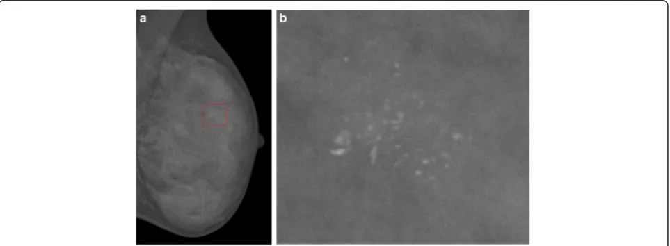
Various types of abnormalities can be observed in mammograms, such as microcalcification clusters and mass lesion, distortion in breast architecture, and asym-metry between breasts which are the most dangerous ones. Microcalcification clusters and mass [5–7] are the most common signs of breast cancer, and microcalcifica-tion (MC) clusters appear in 30–50 % of diagnosed cases. MCs are calcium deposits of very small dimension and appear as a group of granular bright spots in a mammogram. A typical mammogram with microcalcifi-cation clusters is shown in Fig. 1a and the full view of a cluster of microcalcifications in Fig. 1b. Individual MCs are sometimes difficult to detect because of the sur-rounding breast tissue, their variation in shape, and small dimensions.
Computer-aided detection of microcalcification clus-ters has been investigated using many different tech-niques [5, 8]. Roughly speaking, the methods can be classified as traditional enhancement-based method, multiscale analysis, and classifier-based methods. Kim et al. [9] enhanced the mammographic images based on the first derivative (such as Sobel operators and compass operators) and the local statistics.
Laine et al. [10] investigated wavelet multiresolution for mammography contrast enhancement. Three over-complete multiresolution representations were investi-gated. Contrast enhancement was applied for each level separately, and edge features were extracted in each level and decomposition coefficients were modified based on edge features. Final images were reconstructed with modified coefficients. Improved contrast for irregular structures such as microcalcification was observed on their experiments. In our previous work [11], a new
wavelet-based image enhanced method is proposed. A multiscale measure which matches the human vision system is proposed and used to modify wavelet coeffi-cients. The degree of enhancement can be adjusted by manipulating a single parameter. Ramirez-Cobo et al. [12] used 2D wavelet-based multifractal spectrum for malignant and normal classification.
Several machine learning methods have been used for microcalcification detection. El-Naqa et al. [13] investi-gated the support vector machine (SVM) classifier for MC cluster detection, and a successive enhancement learning scheme was proposed to improve the perform-ance. On a set of 76 mammogram images containing 1120 MCs, their method obtained a sensitivity of 94 % with an error rate of one false-positive cluster per image. Ge et al. [14] proposed a system to identify microcalcifi-cation clusters on full-field digital mammograms (FFDMs) with convolution neural network. The system includes six stages: preprocessing, image enhancement with box-rim filter, segmentation of microcalcification candidates, false-positive (FP) reduction for individual microcalcifications with convolution neural network, re-gion clustering, and FP reduction for clustered microcal-cifications. On a dataset of 96 cases with 192 images, they obtained a cluster-based sensitivity of 70, 80, and 90 % at 0.12, 0.61, and 1.49 FPs/image, respectively. Tiedeu et al. [15] detected microcalcifications by inte-grating image enhancement and the threshold-based segmentation method. Several features were extracted for each region from the enhanced image, and by em-bedding feature clustering in the segmentation, their method obtained much less false positives than other methods. Experiments were performed on a dataset of 66 images containing 59 MC clusters and 683 MCs, and high sensitivity (100 %) was obtained, balanced by a
lower specificity (87.77 %). In the work of Oliver et al. [16], the individual microcalcification detection is based on local image features of the microcalcifications from a bank of filters. A pixel-based boosting classifier is then trained, and salient features were selected. Clusters are found by inspecting the local neighborhood of each microcalcification. Malar et al. [17] utilized wavelet-based texture features and the extreme learning machine (ELM) for microcalcification detection and classification. One hundred and twenty regions of interest (ROIs; with 32 × 32 pixels) extracted from the MIAS [18] dataset are used for the experiments. They obtained a classification accuracy of 94 %.
Most of the previous microcalcification detection works have been performed on film-scanned mammo-grams. With the development of the imaging technique, FFDMs have been widely deployed, and they have better image quality than film-scanned images. We will con-centrate on FFDM images.
In this paper, we proposed a novel weighted support vector machine-based microcalcification cluster detec-tion method for FFDM images. Inspired by the work in [19], the possibilistic fuzzy c-means (PFCM) clustering algorithm is used to derive weights for the samples. Sev-eral features are extracted and used to train SVM. The proposed method is evaluated on a publically available FFDM dataset [20], consisting of 410 images.
The contributions of the paper are as follows: (1) The weighted SVM is for the first time introduced for MC and MC cluster detection. (2) A novel weighting scheme based on PFCM clustering is introduced to assign weights to samples; unlike the traditional transductive learning-based “pseudo training dataset generating” method, this integration is more simple and principled. (3) A mutual information criterion-based feature selec-tion is investigated for the MC detecselec-tion in FFDM, and until now, only very few MC detection works have been done on the FFDM dataset.
The rest of the paper is organized as follows: Section 2 introduces the related PFCM technique used, and our method is introduced in Section 3. Experimental results are shown in Section 4. The conclusions and discussions are provided in Section 5.
2 Brief introduction of PFCM clustering
The PFCM is a recently developed clustering algorithm, which has the advantages of the fuzzy c-means (FCM) as well as the possibilistic c-means (PCM) [21] algorithm. Outlier sensitivity is one shortcoming of the FCM clus-tering. The PCM clustering algorithm [21] can overcome the shortcoming, and it can identify the degree of typic-ality that a sample has with respect to the group to which it belongs. However, sometimes the prototypes of PCM clusters can coincide, and the PCM will fail in
these cases. Pal et al. proposed a hybridized PFCM clus-tering [22] to cope with the above shortcomings.
For an unlabeled dataset X= {x1,x2,…,xn}∈Rp, a
c-partition of X is a set of (cn) values {uik} that can be
written as a (c×n) matrix U= [uik], i= 1,…,c, k= 1,…,
n. The possibilistic and fuzzy c-partitions of X are de-fined as [22]
The optimization function in PFCM is formulated as [22]
values of a and b represent the relative importance of membership and typicality values in the computation of the prototypes. The parameters m and η represent the absolute weight of the membership value and typicality value, respectively. One can set b>a and m>η to re-duce the sensitivity to outliers.
The probability (memberships, or relative typicalities, used in FCM) and possibilities (or absolute typicalities, used in PCM) are different. The membershipuikfor data
xkbelongs to a classciwhich is a function ofxkand allc
centroids {v1,…,vk}, while the typicality value is a
func-tion of xk and the center vi alone, as shown below. For
example, in a two-class clustering problem, for a noise data point, which is far away from both clusters, the membership to both cluster uik will be about 0.5
(required by X 2
i¼1
uik¼1), while the typicality values to
both cluster tik will be near zero. For another point
which lies between the two clusters (not far away from the centers), theuikwill also be about 0.5, but the
typic-ality valuestikwill be a positive number not approaching
zero. The probability and typicality can convey different information about the dataset.
PFCM theorem [22]: If DikA=‖xk−vi‖> 0, for everyi,
k, m> 1, η> 1, and if X contains at least c distinct data points, then (U,T,V)∈Mfcm×Mpcm×ℜc×nmay minimize
uik¼
Xc
j¼1
DikA DjkA
2=ðm−1Þ!−1
; 1≤i≤c; 1≤k≤n ð4Þ
tik¼
1
1þ b
γiD
2 ikAi
1=ðη−1Þ; 1≤i≤c; 1≤k≤n ð5Þ
vi¼
Xn
k¼1
aumikþbtηik
xk=
Xn
k¼1
aumikþbtηik
; 1≤i≤c
ð6Þ
γi¼K
Xn
k¼1
umikkxk−vik2
Xn
k¼1
μm ik
ð7Þ
The iterative process of the algorithm is presented in [22].
3 Proposed method
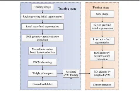
The workflow of the proposed method is shown in Fig. 2. For each image, suspicious MC regions are extracted with active contour segmentation. Then geometry and texture features are extracted for each suspicious MC, a
mutual information-based supervised criterion is used to select important features, and then PFCM is applied to cluster the samples into two clusters. Weights of the samples are calculated based on possibilities and typical-ity values from the PFCM, and the ground truth labels. A weighted nonlinear SVM is trained. During the test process, when an unknown image is presented, a similar process is performed. Suspicious regions are located by active contour segmentation, selected features are ex-tracted, and the suspicious MC regions are classified by the more powerful weighted nonlinear SVM. Finally, the MC regions are analyzed with spatial information to lo-cate MC clusters.
3.1 Level set-based MC segmentation
The segmentation of MC consists of two steps: firstly, several edge points are detected and used to initialize the MC segmentation, and then an active contour is used to refine the initial segmentation. The initial step follows the method proposed in [23]. For a given image
f(x,y), the edge of a microcalcification to be segmented is a closed contour around a known pixel (x0,y0), which is the location of the local highest grayscale value pixel. For each pixel, a slope values(x,y) referred tof(x0,y0) is defined as [23]
ROI geometry, texture feature extraction
Mutual information based feature selection
New image
Region growing initial segmentation
Level set refined segmentation
PFCM clustering
Weight of samples
Ground truth label
Weighted SVM training
ROI geometry, texture feature
extraction
ROI classify by weighted SVM
Cluster detection Training image
Region growing initial segmentation
Level set refined segmentation
Training stage
Testing stage
s xð ;yÞ ¼f xð 0;y0Þ−f xð ;yÞ d xð 0;y0;x;yÞ
ð8Þ
whered(x0,y0,x,y) is the Euclidean distance between the
local maximum pixel (x0,y0) and pixel (x,y). A pixel is
considered on the edge if s(x,y) is maximal along a line segment originating from (x0,y0). The length of the
con-sidered line segment is chosen as 15 (approximately 1 mm as the spatial resolution in INbreast is 70μm per pixel). The line search is applied in 16 equally spaced di-rections originating from the seed pixel. Thus, with each local maximal, 16 edge points are located. Note that the segmentation step will encounter some difficulties for small MC, and the approach used in [24] is adopted to overcome the problem. That is, the segmentation step is performed on the upscaled region containing a possible MC.
For a given local maximal with 16 edge points, a circle is fitted to the points. And the circle is used as the initialization of the level set-based segmentation. Level set originates from the active contour model (snake) [25]. Snake can be edge based or region based.
In this paper, we used the segmentation method we have proposed previously [7, 26]. The final energy func-tional we used is
Eðϕ;f1;f2Þ ¼λ1 Z Z
Kσðx−yÞjI yð Þ−f1ð Þxj 2
Hðϕð Þy Þdy
dx
þλ2 R
ðRKσðx−yÞjI yð Þ−f2ð Þxj 2ð
1−Hðϕð ÞyÞÞdyÞdx þγ1
Z
I xð Þ−c1
j j2
1−Hðϕð ÞxÞ ð Þdxþγ2
Z
I xð Þ−c2
j j2
Hðϕð ÞxÞdx þμZ j∇Hðϕð ÞxÞjdxþv
Z
gδ ϕð Þj∇ϕjdxþw
Z
1 2j∇ϕð Þxj
2− 1
dx
ð9Þ
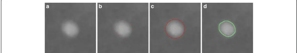
For details about the above function and the numerical implementation, please refer to [7, 26, 27] (see Fig. 3 for an illustration of the segmentation steps).
3.2 Feature extraction from ROI
After segmenting suspicious MC from the ROI, we com-pute a set of geometry and texture features related to the boundary and the region. Several features used here
have been used in our previous work [7] for mass diagnosis.
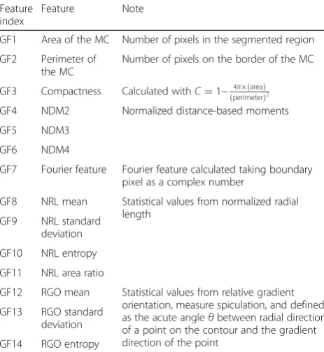
3.2.1 Geometry features
Fourteen geometry features are considered in the study, including area (denoted as GF1, where GF means geom-etry feature), perimeter (GF2), compactness (C, GF3), normalized distance moment (NDM2, NDM3, NDM4, GF4-F6) [28], Fourier feature (FF, GF7) [28], normalized radial length (NRL)-based features (μNRL, σNRL, ENRL,
ARNRL, GF8-GF11) [29], and relative gradient orientation (RGO)-based features (μRGO, σRGO, ERGO, GF12-GF14) [30]. The area is computed by the pixels in the seg-mented region, and the perimeter is computed by the number of pixels on the boundary. C is a measure of contour complexity versus the enclosed area and is defined as C¼1− 4πðareaÞ
perimeter
ð Þ2. For details about geometry features, please see our previous work [7] and the refer-ences therein. The 14 geometry features are listed in Table 1.
3.2.2 Texture features
Besides the shape information of a MC contour, the tex-ture information of the region surrounding the suspi-cious MC boundary also contains important information for MC analysis [8]. Thus, texture features are also used for MC detection. For each suspected MC, a patch with size 16 × 16 is extracted [14, 31], whose center is deter-mined by the center of the suspected MC. Besides the average grayscale in the segmented region in a block (denoted as TF1, where TF means texture feature) (16 × 16 window) and the grayscale difference between the average suspicious region and background (TF2) (the window without taking into account the segmented region), the gray level co-occurrence matrix (GLCM) [32, 33] and wavelet texture features are also extracted.
GLCM has been widely used in mammographic micro-calcifications [8] and masses [34]. We use several GLCM features, including autocorrelation (TF3), contrast (TF4), correlation (TF5), cluster prominence (TF6), cluster shade (TF7), energy (TF8), entropy (TF9), homogeneity (TF10), maximum probability (TF11), sum of squares
(TF12), sum average (TF13), sum variance (TF14), sum entropy (TF15), difference variance (TF16), difference entropy (TF17), information measure of correlation (TF18, TF19), inverse difference normalized (TF20), and inverse difference moment normalized (TF21).
Besides GLCM-based features, we have also extracted several wavelet-based features. Multiscale representa-tions have been widely used in image processing applica-tions. Wavelet analysis is the most common way to generate such a representation [35]. We used undeci-mated wavelet transform with the Daubechies 4 filter for each suspicious MC patch (a 16 × 16 window) in the paper. The entropy and energy of each sub-band are used as features. For an N×N(N= 16) sub-image, nor-malized energy and entropy are computed as follows [24]:
wherexijis theij-th pixel value of the sub-images, and
norm2¼X
Twelve sub-images are generated for each ROI with a three-level wavelet decomposition, and as the first-level
decomposition consists of mostly noise, features are ex-tracted from the levels 2 and 3 sub-bands. Thus, 16 wavelet features are extracted for each ROI and are de-noted with TF22-TF23 from the energy and entropy fea-ture of the level 2 approximation coefficient matrix, and TF24-TF25, TF26-TF27, and TF28-TF29 from horizon-tal, vertical, and diagonal coefficient matrices, respect-ively. TF30-TF37 are defined similarly for level 3 decomposition.
3.3 Feature selection based on mutual information With the above procedure, a lot of features are extracted to represent the possible MC. However, not every fea-ture is useful to discriminate non-MC and MC. Each feature used here has its physical meaning, and it is im-portant to preserve the intelligibility of the result; several methods, such as principal component analysis (PCA) and linear discriminant analysis (LDA) [36], are not applicable.
Feature selection methods can be categorized into two types: filter methods and wrapper methods [37]. The performance of wrapper methods is dependent on the specific classifiers, while the performance of filter methods is usually independent of the classifiers. In this paper, we concentrate on the mutual information (MI)-based filter feature selection method.
Positive (MC) and negative (non-MC) samples are needed to select features. The positive samples are ob-tained with the annotation in the image database, and the negative samples are those ROIs segmented by active contour but do not contain MC. In this way, the selection of non-MC samples is tuned with the whole detection procedure. It is an advantage compared with other commonly used random sample methods, as used in [13].
In information theory, MI calculates the statistical de-pendence between two random variables and can be used to measure the relative utility of each feature to a classification problem. The MI between two random var-iablesXandYis defined as
I Xð ;YÞ ¼
where p(x,y) is the joint probability density function of continual random variables, and p(x) and p(y) are the marginal probability density functions. MI can also be defined with Shannon entropy
I Xð ;YÞ ¼H Xð Þ−H Xð jYÞ ¼H Yð Þ−H Yð jXÞ
¼H Xð Þ þH Yð Þ−H Xð ;YÞ ð14Þ
where H(x) =− ∫p(x)logp(x)dx, H(y|x) =− ∬p(x,y)log
p(y|x)dxdy, and H(x,y) =− ∬p(x,y)logp(x,y)dxdy are the
Table 1Geometry features extracted from a MC boundary
Feature index
Feature Note
GF1 Area of the MC Number of pixels in the segmented region
GF2 Perimeter of
the MC
Number of pixels on the border of the MC
GF3 Compactness Calculated withC¼1− 4πðareaÞ
perimeter
ð Þ2
GF4 NDM2 Normalized distance-based moments
GF5 NDM3
GF6 NDM4
GF7 Fourier feature Fourier feature calculated taking boundary pixel as a complex number
GF8 NRL mean Statistical values from normalized radial length
GF9 NRL standard
deviation
GF10 NRL entropy
GF11 NRL area ratio
GF12 RGO mean Statistical values from relative gradient orientation, measure spiculation, and defined as the acute angleθbetween radial direction of a point on the contour and the gradient direction of the point
GF13 RGO standard
deviation
Shannon entropies. An explanation of MI for feature selec-tion is as follows: LetYbe a variable representing the class label (e.g., MC or non-MC) andXa variable denoting a fea-ture. The entropyH(Y) is known to be a measure of the amount of uncertainty aboutY, whileH(Y|X) is the amount of uncertainty left in Y when knowing an observation X. Therefore, MI can be seen as the amount of information that the measure atXhas about the class labelY. Thus, MI measures the capability of this feature to predict the class label.
As is known, the best ksingle features are usually not the best k combined features, since there may exist re-dundancy between these features. The minimum redun-dancy maximum relevance (mRMR) method [38] considered this problem, and it selects features that have the highest relevance with the target class and are also minimally redundant. Denote the i‐th feature as fi and
the class variable asc. The maximum relevance criterion selects the topmfeatures in the descent order ofI(fi,c),
i.e., the bestmindividual features correlated to the class labels:
Due to feature correlations among features, thembest separated features are not the best combinedmfeatures. The minimum redundancy criteria are introduced to re-move the redundancy among features:
min
The final features are selected sequentially, to select them‐th feature after obtaining them−1 featuresSm−1, by solving the following optimization problem [38]:
max
3.4 Clustering with PFCM and weight samples
With the obtained MC and non-MC samples, using the features selected by the mRMR criterion, PFCM is ap-plied to cluster the samples. Each sample with selected feature values is regarded as a data point. As shown above, for each sample after PFCM clustering, it has a probability and a typicality value.
Letyidenote the label of samplei, and letyi∈{+1,−1}
denote the class variable (MC or non-MC) which we can obtain by the doctor’s manual annotation. Let MUi
denote the probability of sample i belonging to
calcification, let MTþ1i denote the typicality value of sampleibelonging to MC, and letMT−i1 denote the typ-icality value of it belonging to non-MC. MUi, MTþ1i , and MT−i1 can be obtained by PFCM clustering, and their value ranges are between 0 and 1.
We want to give more weights to the samples with higher confidence and define the weightW1ias
W1i¼
the possibility value of it belongs to MC obtained by PFCM is high, the weight W1i is high; otherwise, the
weight is low.
Besides the confidence value, we also used the typical-ity values outputted by PFCM. The weight term consid-ering the typicality value is defined as follows:
W2i¼
For a typical sample belonging to MC or non-MC, its weight W2i is high. For example, for a typical MC
sam-ple xi, the first term inW2i approaches 1, since yi¼1;
MT1i≈1;MT−i1→0 . For a typical non-MC, W2i is also
large due to the second term, while W2i is small for a
noise point, since in this case, bothMTþ1i andMT−i1 ap-proach 0.
We take both possibility information and typical infor-mation into consideration, and the final weight of sam-pleiwe defined is
W3i¼W1iW2i ð20Þ
3.5 Weighted SVM-based classification
Given a set of vectors (x1,…,xn) and their corresponding
labels (y1,…,yn) withyi∈{+1,−1}, the SVM classifier
de-fines a hyperplane (w,b) in kernel space that separates the training data by a maximal margin.
For the weighted SVM, each sample consists of a data vectorxi, a labelyias in standard SVM; besides, a
sam-ple also contains a confidence valuevi. Define the
effect-ive weighted functional margin of weighted sample (xi,
yi,vi) with respect to a hyperplane (w,b) and a margin
normalization functionfto bef(vi)yi(〈w⋅xi〉+b), wheref
is a monotonically decreasing function. To tolerate noise and outliers, more training samples than just those close to the boundary need to be considered.
Definition (margin slack variable) [39]: Given a value
respect to the hyperplane (w,b) and target margin γ is defined to be
ξi¼ max 0ð ;γ−yiðhw⋅xii þbÞÞ ð21Þ
The quantity measures how much a point fails to have a margin γfrom the hyperplane (w,b). If xi is
misclassi-fied by (w,b), then ξi> 0. To generalize the soft margin
classifier to the weighted soft margin classifier, the weighted version of the slack variable is introduced.
Definition (effective weighted margin slack variable) [39]: The effective weighted margin slack variable of a sample (xi,yi,vi) with respect to a hyperplane (w,b) and
margin normalization function f, slack normalization functiong, and target marginγis defined as
ξw
i ¼g vð Þi max 0ð ;γ−yif vð Þi ð<w⋅xi>þbÞÞ
¼g vð Þi ξi ð22Þ
wherefis a monotonically decreasing function such that
f(⋅)∈(0, 1], andg is a monotonically increasing function such thatg(⋅)∈(0, 1].
The weighted SVM optimization problem can be for-mulated as follows: Given a training sample setS= ((x1,
y1,v1),…, (xn,yn,vn)), the hyperplane (w,b) that solves
the following optimization problem
minimizehw⋅wi þCX n
i¼1
g vð Þi ξi
s:t: yiðhw⋅xii þbÞf vð Þi ≥1−ξi;i¼1;⋯;n
ξi≥0;i¼1;⋯;n
ð23Þ
realizes the maximal weighted soft margin hyperplane. If both functionsfandgare set to be constant at 1, then the WSVM coincides with standard SVM.
In the above formulation, the final decision plane will be less affected by those margin-violating samples with low confidence, and samples with high confidence have higher impact on the final decision plane. The optimization problem can be solved using the sequential minimal optimization technique as in standard SVM. The functionf(x) andg(x) are set as used in [39].
4 Experimental results
4.1 Mammogram database
The proposed method was tested on the publically avail-able INbreast database [20]. The database was acquired from the Breast Centre in CHSJ, Porto, between April 2008 and July 2010, and the acquisition equipment was the MammoNovation Simens FFDM. The database has a total of 115 cases (410 images), from which 90 cases are from women with both breasts affected (four images per case) and 25 cases are from mastectomy patients (two images per cases). Several types of lesions (masses, calci-fications, architectural distortion) were included. The pixel size is 70 μm, with 14-bit resolution. The image
matrix was 3328 × 4084 or 2560 × 3328 pixels. All im-ages were saved in DICOM format. The database has a large portion of calcifications. Among the 410 images, calcifications presented in 301 images, and 27 sets of microcalcification clusters occurred in 21 images (≈1.3 clusters per image). A total of 6880 microcalcifications were individually identified in 299 images (≈23.0 calcifi-cations per image).
For our investigation, very small MCs (number of pixels less than 3) are ignored and treated as normal. Note that the tiny MC can be detected with techniques such as wavelet transform. With such criterion, we obtained 2748 MCs on 232 images (≈11.8 MCs per image). Since the MC cluster in this criterion in the dataset is small, and a clus-ter can contain dozens of MC, we used a variant criclus-terion about the MC cluster [40]. That is, a group of objects clas-sified as MCs is considered to be a true-positive (TP) clus-ter only if at least three true calcifications should be detected by an algorithm within an area of 1 cm2. A group of objects classified as MCs is labeled as a FP cluster pro-vided that the objects satisfy the cluster requirement but do not contain true MCs. In this way, 76 MC clusters are defined.
4.2 Results
4.2.1 Segmentation results
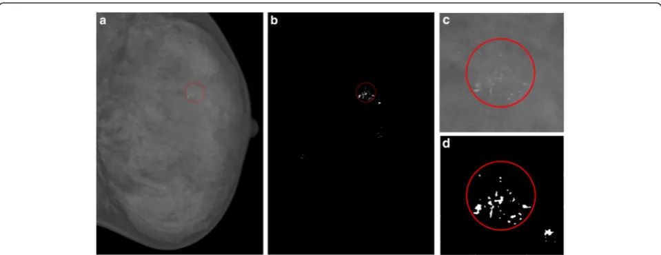
Our method first extracted suspicious MC regions, and then use WSVM to reduce the false positives. If a MC is missed in the segmentation step, then it will not show up in the final detection. Visual inspection of the output im-ages and their corresponding annotations showed that all the MC clusters had been detected in the first segmenta-tion stage. Figure 4 shows the segmentasegmenta-tion stage of an image. In Fig. 4a, the MC cluster is circled. Figure 4b showed the output mask of the first stage, and it can be seen that the MC cluster has been detected correctly. The enlarged parts are shown in Fig. 4c, d.
To quantitatively evaluate the segmentation results, we used Dice coefficient D, which has been widely used for segmentation evaluation. The value of D ranges from 0 (no overlap) to 1 (perfect overlap) and is defined by D
¼ 2ðA∩GÞ
A∩GþA∪G
ð Þ100%, whereAis the region segmented by a method, andGis the manually labeled region. The aver-aged value forDon 100 MC images was 93.8 %, and it in-dicates that the proposed method is accurate for MC segmentation.
4.2.2 Selection of features
only MC cluster) and 88 images not containing MC or MC cluster. That is, in total, 205 images are used for training (containing 1382 MCs, 38 MC clusters, and 2764 non-MCs), and the remaining 205 images (117 im-ages containing MC or MC cluster and 88 imim-ages not containing MC or MC cluster) are used for testing; the test dataset contains 1366 MCs on 116 images and 38 MC clusters on 10 images.
Unlike usually random selection, the non-MC exam-ples are selected considering the initial detection proced-ure. That is, the non-MC examples are selected from the level set segmented regions not containing MC. Thus, the negative examples are specific to the used segmenta-tion method, which is an advantage over the tradisegmenta-tional random selection method. There were 4146 (1382 × 3) training examples in total.
Each MC or non-MC was covered by a 16 × 16 (about 1.12 mm × 1.12 mm with pixel spatial resolution of 0.07 mm) window whose center coincided with the cen-ter of the suspected MC. Geometry features are ex-tracted from the level set segmentation, and GLCM and wavelet texture features are extracted from the window.
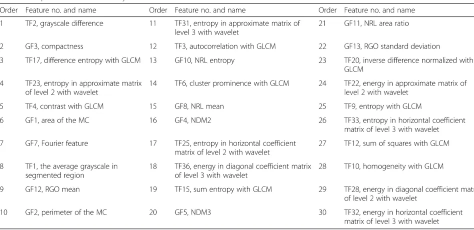
With the extracted features and known class label, MI is used to select the important features. We have ex-tracted 51 features (14 geometry features, 2 grayscale features, 19 GLCM features, and 16 wavelet features) to represent MC and non-MC, and the top 30 features ranked by MI are shown in Table 2.
We used a fivefold cross-validation method to select the number of features; the training samples were equally split into five subsets, four subsets were used as the training dataset and the remaining one subset was used for testing. The averaged performances were recorded to set param-eter values. For the classifier here, we used a standard SVM (with radial basis function kernel) without weights;
more specifically, the LIBSVM toolbox [41] was used. The parametersCandσin the SVM were obtained with cross-validation from set {2−5, 2−4,…, 20,…, 25}. Denote the true-positive number of a classifier as TP, the false-positive number as FP, the true-negative number as TN, and the false-negative number as FN. Then the TPR (true-positive rate), TNR (true-negative rate), and accuracy are defined as TPR¼ TP
TPþFN, TNR¼TNþFPTN , and Accuracy
¼ TPþTN
TPþFNþTNþFN.
Figure 5 shows the classification accuracy with different numbers of features. This figure shows that the accuracy increases with the added features initially, but it begins to decrease after several features are selected, which indicate that some features may degrade the classifier’s perform-ance. The best number of feature used here is 22, and we will use these features in the following experiments. From the features listed in Table 2, we can see selected features including both geometry features and texture features, which indicate that both geometry and texture features are useful to separate MC from non-MC. The top feature is the grayscale difference feature, which is in accordance with the typical characteristic that MC is brighter than the background. The second top feature is the compactness geometry feature, which is also useful to distinguish MC from other bright regions, for example, vessel, since the MC is typically compact while the vessel region is elon-gated. While the other used features may not have a direct explanation, they contain discriminating information for false-positive reduction.
4.2.3 Detection results and comparison with unweighted SVM
samples in the training are clustered and weighted as in Section 3.4. A weighted SVM is trained as introduced in Section 3.5 and then used for testing.
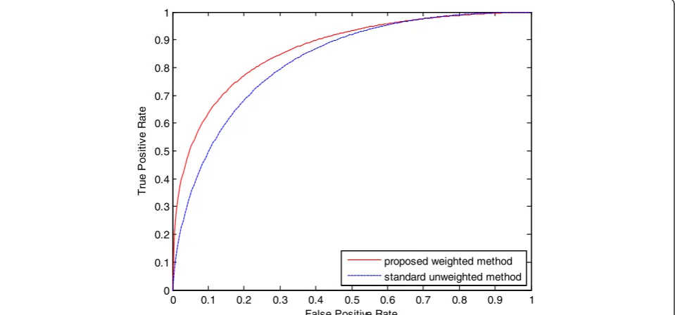
We measured both MC detection and MC cluster de-tection for the experiments. The MC cluster was identi-fied by grouping the objects that have been determined by the algorithm to be MC. The receiver operating char-acteristic (ROC) curves are used to evaluate the per-formance of MC detection, and the free-response receiver operating characteristic (FROC) curves are used
to evaluate the performance of MC cluster detection. The standard SVM without weighting is used to evaluate the effect of the PFCM-based weighting scheme. An ROC curve is a plot of operating points which can be considered as a plot of true-positive rate as a function of false-positive rate. The curve is generated by threshold-ing the output possibilities of MC of the classifier. A FROC curve is a plot of the correct detection rate (true-positive rate) achieved by a classifier versus the average number of false positives (FPs) per image varied over the
Table 2Top 30 features ranked by mutual information filter
Order Feature no. and name Order Feature no. and name Order Feature no. and name
1 TF2, grayscale difference 11 TF31, entropy in approximate matrix of
level 3 with wavelet
21 GF11, NRL area ratio
2 GF3, compactness 12 TF3, autocorrelation with GLCM 22 GF13, RGO standard deviation
3 TF17, difference entropy with GLCM 13 GF10, NRL entropy 23 TF20, inverse difference normalized with
GLCM
4 TF23, entropy in approximate matrix of level 2 with wavelet
14 TF6, cluster prominence with GLCM 24 TF22, energy in approximate matrix of level 2 with wavelet
5 TF4, contrast with GLCM 15 GF8, NRL mean 25 TF9, entropy with GLCM
6 GF1, area of the MC 16 GF4, NDM2 26 TF33, entropy in horizontal coefficient
matrix of level 3 with wavelet
7 GF7, Fourier feature 17 TF25, entropy in horizontal coefficient
matrix of level 2 with wavelet
27 TF12, sum of squares with GLCM
8 TF1, the average grayscale in segmented region
18 TF36, energy in diagonal coefficient matrix of level 3 with wavelet
28 TF10, homogeneity with GLCM
9 GF12, RGO mean 19 TF15, sum entropy with GLCM 29 TF28, energy in diagonal coefficient matrix
of level 2 with wavelet
10 GF2, perimeter of the MC 20 GF5, NDM3 30 TF32, energy in horizontal coefficient
matrix of level 3 with wavelet
2 4 6 8 10 12 14 16 18 20 22 24 26 28 30 32 34 36
0.6 0.65 0.7 0.75 0.8 0.85 0.9 0.95 1
Number of features
A
c
cu
ra
cy
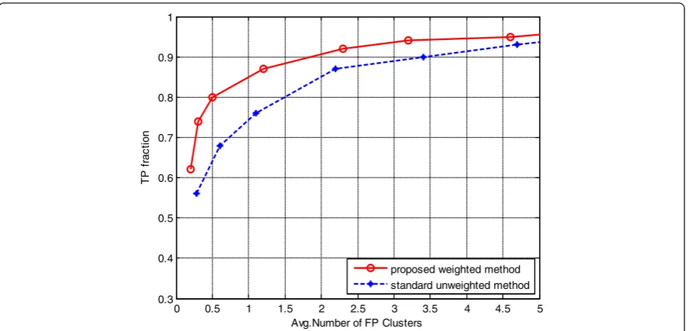
decision threshold. A FROC curve can provide a sum-mary of the trade-off between detection sensitivity and specificity.
We compared the performance of the standard un-weighted SVM and the proposed PFCM clustering-based weighted SVM on MC classification. The test set con-tains 1366 true MCs, and we selected 2732 non-MC samples from the segmentation on test images, similar to the training step. The performance of standard un-weighted SVM and our un-weighted SVM is shown in Fig. 6 with a ROC curve. The AUC (Az), which is the area
under the ROC curve, is used to compare the perform-ance of the two classification methods. The AUC for standard unweighted SVM is 82.68 %, and the AUC of the proposed PFCM-based weighted SVM is 86.76 %. We can see that with the same training samples and test samples, the proposed weight SVM achieved better per-formance than the standard unweighted SVM.
The performances of the proposed weighted SVM ap-proach, along with the standard unweighted SVM, are also presented for MC cluster detection with the FROC curve, as shown in Fig. 7. The proposed method ob-tained a high sensitivity of 92 % with a FP rate of 2.3 FP clusters/image. At a similar sensitivity, the FP rate of the standard unweighted SVM obtained 4.7 FP clusters/ image. It can be seen that the proposed weighted SVM also outperformed the standard unweighted SVM for MC cluster detection.
5 Discussion and conclusion
Automatic detection of microcalcification in mammo-grams has been investigated by many researchers in the
past two decades. In [15], Tiedeu et al. segmented microcalcifications with an adaptive threshold method on the enhanced image, and a set of moment-based geo-metrical features were used for false-positive reduction. On a dataset of 66 images containing 59 MC clusters and 683 MCs, they obtained a sensitivity of 100 % with a low specificity of 87.77 %. They also performed benign/ malignant classification. Oliver et al. [16] extracted image features with a bank of filters, and a boosting method is used to separate MC from non-MC. The data-set they used included the MIAS datadata-set (322 mammo-grams) and another 280 FFDM mammograms. Their method’s performance for MC is Az= 0.85 with ROC
analysis, and for MC clusters, the result is 80 % sensitiv-ity at one false-positive cluster per image.
In [42], Nunes et al. obtainedAz= 0.93 for MC detection
on a database of 121 mammograms by combining three contrast enhancement techniques. Papadopoulos et al. [43] investigated five image enhancement techniques and obtained Az= 0.92 for MC detection on a database
con-sisting of 60 mammograms from the MIAS and Nijmegen databases. Linguraru et al. [44] proposed MC cluster de-tection based on a biologically inspired contrast dede-tection algorithm, integrated with a preprocessing step (curvilin-ear structure removal and image enhancement). They ob-tained a 95 % sensitivity with 0.4 false positives per image on a small subset of the Digital Database for Screening Mammography (DDSM) dataset [45] (82 images, 58 of which contain microcalcification and the other 24 were normal ones, the number of MC cluster is 82). Ge et al. [46] developed two systems to detect microcalcification clusters, one for FFDM and the other one for screen-film
0 0.1 0.2 0.3 0.4 0.5 0.6 0.7 0.8 0.9 1 0
0.1 0.2 0.3 0.4 0.5 0.6 0.7 0.8 0.9 1
False Positive Rate
T
ru
e
Po
s
iti
v
e
R
a
te
proposed weighted method standard unweighted method
mammograms (SFMs). They obtained an average of 0.96 or 2.52 false positives per image at 90 % sensitivity on FFDMs and SFMs, respectively. The FFDM dataset they used includes 96 mammograms with microcalcifications and 108 normal mammograms.
It is hard to directly compare different methods, since the used datasets are different, and the definition for MC cluster sometimes is also different. On the DDSM dataset [45], usually different subsets are used in investi-gations. Most of the above techniques are developed for film-scanned mammograms. Here we developed the method on the FFDMs, as images from FFDM have bet-ter image quality than file-scanned images and are also widely deployed. From the above results, it can be seen that the performance of our method with 92 % sensitiv-ity at 2.3 false-positive clusters per image is better or similar to the above results. It should be noted that our method is investigated on a larger dataset.
In this paper, we proposed a weighted SVM technique for detection of MC clusters in FFDM. In this approach, suspicious MC regions are first segmented with active contour, and then the regions are classified by a trained weighted SVM. The non-MC training samples are se-lected from the segmented regions, which can be better tuned to the whole procedure than random sampling. Mutual information criterion was used to select import-ant features, and among the extracted 51 features, 22 features are selected and used in the training and test process. The training samples are weighted with the pos-sibility and typicality value of a sample belonging to MC output by the novel introduction of possibilistic fuzzy c-means (PFCM) clustering. Experimental results with
ROC and FROC analysis using a set of 410 FFDM mam-mograms demonstrated that the proposed method outperformed the standard unweighted SVM. The proposed weight scheme may be also applicable to other classifiers, such as random forest, and we will investigate these problems in the future. Besides, we will try to adapt the method for traditional film-scanned mammograms.
Competing interests
The authors declare that they have no competing interests.
Acknowledgements
This work is partially supported by the National Natural Science Foundation of China (No. 61403287, No. 61472293, No. 31201121) and the Natural Science Foundation of Hubei Province (No. 2014CFB288).
Received: 1 March 2015 Accepted: 13 July 2015
References
1. GLOBOCAN 2012 v1.0,Cancer Incidence and Mortality Worldwide: IARC CancerBase No. 11 [Internet](International Agency for Research on Cancer, Lyon, France, 2013). Available from: http://globocan.iarc.fr
2. CH Lee, DD Dershaw, D Kopans, P Evans, B Monsees, D Monticciolo, RJ Brenner, L Bassett, W Berg, S Feig, E Hendrick, E Mendelson, C D'Orsi, E Sickles, LW Burhenne, Breast cancer screening with imaging:
recommendations from the Society of Breast Imaging and the ACR on the use of mammography, breast MRI, breast ultrasound, and other technologies for the detection of clinically occult breast cancer. J. Am. Coll. Radiol.7, 18–27 (2010)
3. M Giger, Current issues in CAD for mammography, inDigital Mammography (Elsevier, Philadelphia, 1996), pp. 53–59
4. SV Destounis, P DiNitto, W Logan-Young, E Bonaccio, ML Zuley, KM Willison, Can computer-aided detection with double reading of screening mammograms help decrease the false-negative rate? Initial experience 1. Radiology232, 578–584 (2004)
5. J Tang, RM Rangayyan, J Xu, I El Naqa, Y Yang, Computer-aided detection and diagnosis of breast cancer with mammography: recent advances. IEEE Trans. Inf. Technol. Biomed.13, 236–251 (2009)
0 0.5 1 1.5 2 2.5 3 3.5 4 4.5 5 0.3
0.4 0.5 0.6 0.7 0.8 0.9 1
Avg.Number of FP Clusters
T
P
fr
a
c
ti
o
n
proposed weighted method standard unweighted method
6. X Liu, Z Zeng, A new automatic mass detection method for breast cancer with false positive reduction. Neurocomputing152, 388–402 (2015) 7. X Liu, J Tang, Mass classification in mammograms using selected geometry
and texture features, and a new SVM-based feature selection method. IEEE Syst. J.8, 910–920 (2014)
8. H-D Cheng, X Cai, X Chen, L Hu, X Lou, Computer-aided detection and classification of microcalcifications in mammograms: a survey. Patt. Recog. 36, 2967–2991 (2003)
9. JK Kim, JM Park, KS Song, H Park, Adaptive mammographic image enhancement using first derivative and local statistics. IEEE Trans. Med. Imaging16, 495–502 (1997)
10. AF Laine, S Schuler, J Fan, W Huda, Mammographic feature enhancement by multiscale analysis. IEEE Trans. Med. Imaging13, 725–740 (1994) 11. J Tang, X Liu, Q Sun, A direct image contrast enhancement algorithm in the
wavelet domain for screening mammograms. IEEE J. Sel. Top. Sign. Proces. 3, 74–80 (2009)
12. P Ramírez-Cobo, B Vidakovic, A 2D wavelet-based multiscale approach with applications to the analysis of digital mammograms. Comput. Stat. Data. An. 58, 71–81 (2013)
13. I El-Naqa, Y Yang, MN Wernick, NP Galatsanos, RM Nishikawa, A support vector machine approach for detection of microcalcifications. IEEE Trans. Med. Imaging21, 1552–1563 (2002)
14. J Ge, B Sahiner, LM Hadjiiski, HP Chan, J Wei, MA Helvie, C Zhou, Computer aided detection of clusters of microcalcifications on full field digital mammograms. Med. Phys.33, 2975–2988 (2006)
15. A Tiedeu, C Daul, A Kentsop, P Graebling, D Wolf, Texture-based analysis of clustered microcalcifications detected on mammograms. Digit. Signal Process.22, 124–132 (2012)
16. A Oliver, A Torrent, X Lladó, M Tortajada, L Tortajada, M Sentís, J Freixenet, R Zwiggelaar, Automatic microcalcification and cluster detection for digital and digitised mammograms. Knowl.-Based Syst.28, 68–75 (2012) 17. E Malar, A Kandaswamy, D Chakravarthy, A Giri Dharan, A novel approach
for detection and classification of mammographic microcalcifications using wavelet analysis and extreme learning machine. Comput. Biol. Med.42, 898–905 (2012)
18. J Suckling, J Parker, DR Dance, S Astley, I Hutt, C Boggis, I Ricketts, E Stamatakis, N Cerneaz, SL Kok, P Taylor, D Betal, J Savage, The mammographic image analysis society digital mammogram database, in Exerpta Medica. International Congress Series, (Excerta Medica, Amsterdam 1994), pp. 375–378
19. J Quintanilla-Domínguez, B Ojeda-Magaña, A Marcano-Cedeño, MG Cortina-Januchs, A Vega-Corona, D Andina, Improvement for detection of microcalcifications through clustering algorithms and artificial neural networks. EURASIP J. Adv. Sig. Proc.2011, 91 (2011)
20. IC Moreira, I Amaral, I Domingues, A Cardoso, MJ Cardoso, JS Cardoso, INbreast: toward a full-field digital mammographic database. Acad. Radiol. 19, 236–248 (2012)
21. R Krishnapuram, JM Keller, A possibilistic approach to clustering. IEEE Trans. Fuzzy Syst.1, 98–110 (1993)
22. NR Pal, K Pal, JM Keller, JC Bezdek, A possibilistic fuzzy c-means clustering algorithm. IEEE Trans. Fuzzy Syst.13, 517–530 (2005)
23. IN Bankman, T Nizialek, I Simon, OB Gatewood, IN Weinberg, WR Brody, Segmentation algorithms for detecting microcalcifications in mammograms. IEEE Trans. Inf. Technol. Biomed.1, 141–149 (1997)
24. H Soltanian-Zadeh, F Rafiee-Rad, S Pourabdollah-Nejad D, Comparison of multiwavelet, wavelet, Haralick, and shape features for microcalcification classification in mammograms. Patt. Recog.37, 1973–1986 (2004) 25. M Kass, A Witkin, D Terzopoulos, Snakes: active contour models. Int. J.
Comput. Vision1, 321–331 (1988)
26. J Tang, X Liu, Classification of breast mass in mammography with an improved level set segmentation by combining morphological features and texture features, inMulti Modality State-of-the-Art Medical Image
Segmentation and Registration Methodologies(Springer, New York, 2011), pp. 119–135
27. C Li, C-Y Kao, JC Gore, Z Ding, Minimization of region-scalable fitting energy for image segmentation. IEEE Trans. Image Processing17, 1940–1949 (2008) 28. L Shen, RM Rangayyan, JL Desautels, Application of shape analysis to
mammographic calcifications. IEEE Trans. Med. Imaging13, 263–274 (1994) 29. J Kilday, F Palmieri, M Fox, Classifying mammographic lesions using
computerized image analysis. IEEE Trans. Med. Imaging12, 664–669 (1993)
30. B Sahiner, H-P Chan, N Petrick, MA Helvie, LM Hadjiiski, Improvement of mammographic mass characterization using spiculation measures and morphological features. Med. Phys.28, 1455–1465 (2001)
31. J Fu, S-K Lee, ST Wong, J-Y Yeh, A-H Wang, H Wu, Image segmentation feature selection and pattern classification for mammographic microcalcifications. Comput. Med. Imaging Graph.29, 419–429 (2005) 32. RC Gonzalez, RE Woods,Digital Image Processing(Prentice Hall, New Jersey, 2002) 33. R Haralick, I Dinstein, K Shanmugam, Textural features for image
classification. IEEE Trans. Syst. Man Cybern.3, 610–621 (1973) 34. X Liu, J Liu, D Zhou, J Tang, A benign and malignant mass classification
algorithm based on an improved level set segmentation and texture feature analysis, in2010 4th International Conference on Bioinformatics and Biomedical Engineering (iCBBE), Chengdu, 18-20 June 2010, pp. 1–4 35. S Mallat,A Wavelet Tour of Signal Processing(Academic Press, New York, 1999) 36. RO Duda, PE Hart, DG Stor,Pattern Classification(Wiley, New York, 2001) 37. R Kohavi, GH John, Wrappers for feature subset selection. Artif. Intell.97,
273–324 (1997)
38. H Peng, F Long, C Ding, Feature selection based on mutual information criteria of max-dependency, max-relevance, and min-redundancy. IEEE Trans. Patt. Anal. Mach. Int.27, 1226–1238 (2005)
39. X Wu, R Srihari, Incorporating prior knowledge with weighted margin support vector machines, inProceedings of the Tenth ACM SIGKDD, 2004, pp. 326–333
40. M Kallergi, GM Carney, J Gaviria, Evaluating the performance of detection algorithms in digital mammography. Med. Phys.26, 267–275 (1999) 41. C-C Chang, C-J Lin, LIBSVM: a library for support vector machines. ACM T.
Intel. Syst. Tec.2, 1–27 (2011)
42. FL Nunes, H Schiabel, CE Goes, Contrast enhancement in dense breast images to aid clustered microcalcifications detection. J. Digit. Imaging20, 53–66 (2007)
43. A Papadopoulos, DI Fotiadis, L Costaridou, Improvement of microcalcification cluster detection in mammography utilizing image enhancement techniques. Comput. Biol. Med.38, 1045–1055 (2008) 44. MG Linguraru, K Marias, R English, M Brady, A biologically inspired algorithm
for microcalcification cluster detection. Med. Image Anal.10, 850–862 (2006) 45. M Heath, K Bowyer, D Kopans, R Moore, P Kegelmeyer, The digital database
for screening mammography, inProceedings of the 5th International Workshop on Digital Mammography, 2000, pp. 212–218
46. J Ge, LM Hadjiiski, B Sahiner, J Wei, MA Helvie, C Zhou, HP Chan, Computer-aided detection system for clustered microcalcifications: comparison of performance on full-field digital mammograms and digitized screen-film mammograms. Phys. Med. Biol.52, 981–1000 (2007)
Submit your manuscript to a
journal and benefi t from:
7Convenient online submission 7Rigorous peer review
7Immediate publication on acceptance 7Open access: articles freely available online 7High visibility within the fi eld
7Retaining the copyright to your article