A new frequency approach for light flicker evaluation in electric power systems

R E S E A R C H

Open Access

A new frequency approach for light flicker

evaluation in electric power systems

Luigi Feola

, Roberto Langella and Alfredo Testa

Abstract

In this paper, a new analytical estimator for light flicker in frequency domain, which is able to take into account also the frequency components neglected by the classical methods proposed in literature, is proposed. The analytical solutions proposed apply for any generic stationary signal affected by interharmonic distortion. The light flicker analytical estimator proposed is applied to numerous numerical case studies with the goal of showing i) the correctness and the improvements of the analytical approach proposed with respect to the other methods proposed in literature and ii) the accuracy of the results compared to those obtained by means of the classical International Electrotechnical Commission (IEC) flickermeter. The usefulness of the proposed analytical approach is that it can be included in signal processing tools for interharmonic penetration studies for the integration of renewable energy sources in future smart grids.

Keywords:Light flicker; IEC flickermeter; Interharmonic; Distributed energy resources; Power quality; Smart grids

1 Introduction

Light flicker (LF) phenomenon is still considered one of the most important power quality (PQ) problems due to its ability to be directly perceived by customers, produ-cing complaints from them.

LF is caused by the modulation of the supply funda-mental voltage, which produces modulated light emis-sions whose severity, in terms of annoying effects on humans, depends on modulation amplitudes and fre-quencies as well as on lamp technologies [1]. LF is commonly measured by means of the International Electrotechnical Commission (IEC) flickermeter [2] that, for historical reasons, was designed and tested only with reference to voltage amplitude modulation (AM), which was the first source of LF identified and refer-ring only to 60-W incandescent bulbs, which were the most diffused lamps all over the word at that time.

Today, incandescent lamps are going to be banned, in particular in Europe, Australia and North America, but the IEC flickermeter is still the only instrument used also because international standards are based on it.

The main drawbacks of the IEC flickermeter are as follows: i) it is based on the incandescent bulb model; ii) it requires 10 min of time domain signals to give the short-term flicker sensation index output, Pst; and iii) the output data cannot be used to study LF propagation effects in distribution and transmission networks.

Basic literature demonstrates the perfect equivalence of amplitude modulation to the summation of interhar-monic tones of proper amplitudes and phase angles superimposed to the fundamental [3].

Starting from the beginning of the last decade, sev-eral papers aimed to model the IEC flickermeter in the frequency domain have been written [4-13]. Some of them [4,7,10,11] are pure frequency domain methods. Some others [6,9,12] are hybrid time-frequency do-main methods.

Mayordomo et al. obtained very accurate analytical formulas that were applied to the voltages of DC and AC electrical arc furnace (EAF) measurements. In [13], the analytical formulas have been used to evaluate the propagation in the network of flicker produced by rapidly varying loads. In [11], a spectral decomposition-based ap-proach is proposed to estimate LF caused by EAFs where

* Correspondence:luigi.feola@unina2.it

Department of Industrial and Information Engineering, Second University of Naples, DIII-SUN, Via Roma, 29, 81031 Aversa, Caserta, Italy

the system frequency deviates significantly due to the EAF operation. Both methods start from the discrete Fourier transform (DFT) performed over 200 ms, which is perfectly compatible with the IEC Standard 61000-4-7 [14] that defines harmonic and interharmo-nic measurement techniques.

All of the above-mentioned methods are based on simplified assumptions essentially based on the con-cept that, due to the design specifications of the filters of the IEC flickermeter, the interharmonic compo-nents below 15 Hz and above 85 Hz can be neglected, with reference to 50 Hz systems. This assumption is demonstrated to be valid when the interharmonic source is an EAF which mainly produces modulation of the fundamental voltage in the frequency range from 0 to 20 Hz, that is to say modulations produced by interharmonics in the frequency range from 20 to 80 Hz. Recent studies have demonstrated that modern distributed energy resources, in particular wind tur-bines, are able to produce interharmonics in a wide range of frequency from DC to some kilohertz [15]. Moreover, in [16-18], it was demonstrated that inter-harmonic components produced by adjustable speed drives can cover all the frequency range from DC.

In this paper, the above-mentioned simplified as-sumption is overcome, leading to analytical solutions, of different complexities, able to take into account also the frequency components neglected by the classical methods. The analytical solutions proposed apply for any generic stationary signal affected by interharmonic distortion. The LF analytical estimator proposed is applied to numerous numerical case stud-ies with the goal of showing i) the correctness and the improvements of the analytical approach proposed with respect to the other methods proposed in litera-ture and ii) the accuracy of the results compared to those obtained by means of the classical IEC flicker-meter. The usefulness of the proposed analytical approach is that it can be included in signal processing tools for interharmonic penetration studies for the integration of renewable energy sources in future smart grids.

2 Analytical assessment of IEC flickermeter response due to interharmonics

In this section, the behaviour of the IEC flickermeter in terms of instantaneous flicker sensation (PU), that is the output of the block 4 of the IEC flickermeter (Figure 1), is analytically assessed.

The analytical solutions proposed apply for any generic stationary signal affected by interharmonic distortion. The generic signal is decomposed intoNinterharmonic pairs. Each pair is constituted of two tones in symmetrical frequency positions with respect to the fundamental fre-quency. Moreover, each of two components of the pair has generic amplitude and generic phase angle. Obviously, the case of single interharmonic components can be easily obtained assuming the amplitude of one of the two com-ponents of the pair equal to zero.

Here, explicit reference is made to 50-Hz systems, but the considerations developed may also be ap-plied to 60-Hz systems by changing the constants and parameters.

2.1 Single pair

A normalized voltage with a couple of superimposed inter-harmonic tones (N= 1) in symmetrical angular frequency positions (lower and upper) with respect to the fundamen-tal signal (ω1_L=ω1 – Δω1 and ω1_U=ω1+Δω1) can be expressed as:

u tð Þ ^

u ¼a0cosðω1tþφ1Þ

þa1 Lcos½ðω1−Δω1Þtþφ1 L

þa1 Ucos½ðω1þΔω1Þtþφ1 U; ð1Þ

withûrepresenting the half cycle rms value processed through a first-order filter with a time constant of 27.3 s; a0, ω1 and φ1, respectively, representing the relative amplitude, the angular frequency and the

phase angle of the fundamental tone; a1_L and a1_U

representing the relative amplitudes of the

interhar-monic tones and φ1_L and φ2_L representing their

phase angles, respectively.

The squaring of (1) (block 2 in Figure 1) yields a demo-dulated signal that is very close to the luminous fluxΦ:

u tð Þ

^

u

2

¼1 2 a

2

0þa21 Lþa21 U

þ1 2

a20cos 2ð ω1tþ2φ1Þ þa21 Lcos 2½ ðω1−Δω1Þtþ2φ1 L

þa2

1 Ucos 2½ ðω1þΔω1Þtþ2φ1Ug

þa0a1 LfcosðΔω1t−φ1 Lþφ1Þþcos 2½ðω1−Δω1Þtþφ1 Lþφ1g

þa0a1 UfcosðΔω1tþφ1 Uþφ1Þ þcos 2½ðω1þΔω1Þtþφ1 Uþφ1g

þa1 La1 U½cos 2ð Δω1t−φ1 Lþφ1 UÞ þcos 2ðω1tþφ1 Lþφ1 UÞ;

ð2Þ

Block 3 is composed of a cascade of two filters. The first is used to eliminate the DC component and the component at twice the fundamental frequency present at the output of the demodulator. This filter is composed of a cascade of a high-pass filter (HPF) of first order with a cutoff frequency of 0.05 Hz and a Butterworth low-pass filter (LPF) of the sixth order with a cutoff frequency of 35 Hz for 230 V/50 Hz systems. The sec-ond is used to weigh the voltage fluctuation according to the lamp-eye-brain sensitivity. The transfer functions and the Bode diagrams for these filters are reported in (3) and (4) and in Figure 2 together with their product G(s) =X(s)F(s).

X sð Þ ¼ s sþωHPF

n0

s6_þd5s5_þd4s4_þd3s3_þd2s2_þd1sþd0;

ð3Þ

F sð Þ ¼ kω1s s2_þ2λsþω2

1

1þs=ω2

1þs=ω3

ð Þð1þs=ω4Þ;

ð4Þ

being the coefficient ofX(s) andF(s) shown in Table 1 and in Table 2, respectively [2].

Under the hypothesis that block 3 gates the DC com-ponent and all the comcom-ponents at a frequency certainly higher than 100 Hz (frequencies greater than the cutoff frequency of 35 Hz) and consideringG(s) =X(s)F(s) the output of the block 3 is:

ΔΦ≅H

GΔω1

j ja0a1 LcosðΔω1t−φ1 Lþφ1þ∠GΔω1Þ þ jGΔω1ja0a1 UcosðΔω1tþφ1U−φ1þ∠GΔω1Þ þjG2Δω1ja1 La1 Ucos 2ð Δω1t−φ1 Lþφ1 Uþ∠G2Δω1Þ þjG2ω1−Δω1ja0a1 Lcos 2½ð ω1−Δω1Þtþφ1 Lþφ1þ∠G2ω1−Δω1

þjG2ω1−2Δω1j a2

1 L

2 cos 2½ ðω1−Δω1Þtþ2φ1 Lþ∠G2ω1−2Δωg; ð5Þ

where H¼pffiffiffiffiffiffiffiffiffiffiffiffiffiffiffiffiffi1238400 is a gain factor related to the normalization of the weighting curve, and four different magnitude and phase gains GΔω1;G2Δω1;G2ω1−Δω1 and

G2ω1−2Δω1 are introduced for the five components

de-pending on their angular frequency distances.

Block 4 of the flickermeter squares and filters the in-put signal. The filtering is obtained by means of a low-pass filter with a cutoff frequency of 0.5305 Hz and transfer function equal to:

0 10 20 30 40 50 60 70 80 90 100 -120

-100 -80 -60 -40 -20 0

Frequency (Hz)

)

B

d(

e

d

uti

n

g

a

M

X(s) F(s) X(s)*F(s) X(s)

F(s)

G(s)=F(s)*X(s)

Y sð Þ ¼ 2π0:5305

sþ2π0:5305: ð6Þ

This filter has the goal to attenuate all the sinusoidal components, leaving the continuous component un-affected. Although the bandwidth of the filter is very nar-row, not all the sinusoidal components may be void. For this reason, the instantaneous flicker sensation due to the single interharmonic pair can be written as:

PU1ð Þ ¼t PU1 DCþPU1 ACð Þt ; ð7Þ

where PU1_DCand PU1_AC(t) are the DC and the residual AC component of the instantaneous flicker sensation, respectively.

With reference only to the DC component of PU1and applying at the block 4 the signal (5), it is possible to demonstrate that:

PU1 DC¼PU1 DC1þPU1 DC2; ð8Þ

where PU1_DC1and PU1_DC2are equal, respectively, to:

PU1 DC1≅

As it will be shown in a more comprehensive manner in the following sections, the first component (9) as-sumes prevalent values for all the values of Δω1 while the second (10) assumes values increasingly larger how close is the frequency of the lower interharmonic tone to zero.

It is worth noting that (9) corresponds to the analo-gous expressions reported in [7] and in [10]. The differ-ence is that in cited referdiffer-ences, the filter X(s) was considered ideal, that is to say that G(s)= X(s)F(s)= F(s); so (9) considers the red curve of Figure 2 instead of the green one considered in [7] and in [10].

With reference only to the residual AC component of PU1and applying at the block 4 the signal (5), it is pos-sible to demonstrate that:

PU1 ACð Þ ¼t PU1 AC1ð Þ þt PU1 AC2ð Þt ; ð11Þ

where PU1_AC1and PU1_AC2, considering only the

com-ponent of major interest, are equal, respectively, to:

PU1 AC1ð Þt ≅PU1 AC1Δω1ð Þ þt PU1 AC1 2Δω1ð Þt

PU1_AC1 and PU1_AC2 are oscillating components due to the summation of sinusoidal signals with different an-gular frequencies (the anan-gular frequency of each sum-mand is indicated in the subscript). In particular, PU1_AC1assumes higher values how closeΔω1is to zero, while PU1_AC2 assumes higher values how close Δω1is to the fundamental angular frequency.

For the sake of brevity, the analytical assessment of the summands of (12) and (13) are reported extensively in Appendix A.

2.2 Two pairs

A normalized voltage with two pairs of superimposed interharmonic tones in symmetrical frequency positions (Δω1 and Δω2) with respect to the fundamental signal can be expressed as:

u tð Þu^¼a0cosðω1tþφ1Þ þa1 Lcos½ðω1−Δω1Þtþφ1 L

relative amplitudes and the phase angles of the first interharmonic pair, respectively, and a2_L and a2_U

and φ2_L and φ2_U of the second interharmonic pair,

respectively.

Using the same procedure used for the single pair of interharmonic tones (shown in Section 2.1) and neglect-ing the effect on the AC component of the instantan-eous flicker sensation of the interaction between the two interharmonic pairs, it is possible to demonstrate that:

PU1þ2¼PU1þPU2þPU12 DC¼PU1 DCþPU1 AC

interharmonic pair tones and PU12_DC is the DC

com-ponent of instantaneous flicker sensation due to the interaction between the two interharmonic pairs. For sake of brevity, the analytical assessment of PU12_DCis

reported in Appendix B. Again, as in (7), two different components, one DC (PU1+2_DC) and the other AC

(PU1+2_AC), are defined.

From the previous formulas, it should be noted that in case of two interharmonic couples superimposed to the fun-damental signal, the PU is not only due to the sum of the contributions to the instantaneous flicker sensation of the single interharmonic pair, but there is also a component due to the combination effect of the interharmonic pairs. The en-tity of this effect will be evaluated in the following sections.

2.3Npairs

Starting from the analytical assessments of Section 2.2, it is possible to generalize the analytical assessment to the case of N pairs of interharmonic tones. In fact, from (15), it is possible to obtain:

PUTOT¼

where PUTOT_DC and PUTOT_AC are the DC and

the AC components, respectively, of the instantaneous flicker sensation due to N symmetric interharmonic pairs superimposed to the fundamental signal.

3 Numerical case studies

In this section, different numerical case studies are shown to validate the analytical assessment presented in Section 2. The results obtained by a numerical im-plementation of the IEC flickermeter (according with the standard IEC 61000-4-15) and the results obtained by the formulas of the analytical flickermeter pre-sented in this paper, both implemented in MATLAB, are compared. The block diagram of the numerical case studies is shown in Figure 3.

The steps performed to obtain the results of each nu-merical case study are as follows:

1. A time domain signal with a length of 10 min with different characteristics, according with the case study, is generated.

2. The signal is analysed by means of the IEC flickermeter, which returns both the reference of the instantaneous flicker sensation and of

the short-term flicker severity value, PUrefand

Pst_ref, respectively.

3. A DFT is performed only on the Fourier period of

the signal-generated [1] since the signal is stationary

in terms of fundamental and interharmonic signals in all the 10 min.

4. The output of the DFT is analysed by means

of the analytical formulas of Section2,

according with the case study, to obtain the value of instantaneous flicker sensation (PU). 5. The instantaneous flicker sensation is used as

input to the statistical evaluation (like that described in the Standard IEC 61000-4-15)

to obtain the short-term flicker severity (Pst).

6. The values of PUref,Pst_ref, PU andPstso obtained

have been post-processed to calculate the error of the analytical estimation.

DFT _EstimationsAnalytical Statistical Evaluation

3.1 Single pair producing AM

The interharmonic pairs have modulation frequencies varying between 0.1 and 49.9 Hz with steps of 0.1 Hz. For each modulation frequency, the amplitude of the pair taken from Figure 4, where the interharmonic amplitudes of pairs of symmetric interharmonic

tones superimposed to the fundamental causing a Pst equal to 1 versus the lower interharmonic frequency of the pair, is shown. Furthermore, it should be noted that since the Fourier period of the signal generated is 10 s, a DFT with a spectral resolution of 0.1 Hz is used.

0 5 10 15 20 25 30 35 40 45 50 0

1 2 3 4 5 6 7 8

Lower Interharmonic Frequency (Hz)

)

%(

e

d

uti

l

p

m

A

Figure 4Amplitudes of pairs of symmetric interharmonics causing unitary_Pstversus the pair lower interharmonic frequency.

0 5 10 15 20 25 30 35 40 45 50

0 5 10 15 20 25 30 35 40

X: 48.1 Y: 5.051

Lower Interharmonic Frequency (Hz)

P

f

o

n

oit

a

mit

s

E

ni

r

orr

E

st

)

%(

X: 20.8 Y: 5.157 X: 6.2

Y: 5.368 X: 0.8 Y: 5.734

X: 49.8 Y: 3.671

P_stBASE P

st I

P

st II

P

st III BASE

st

P1

III st

P

II st

P

st

P

Three different analytical estimations of the instantan-eous Flicker sensation, with decreasing complexity, have been considered:

I) PUI

1¼PU1¼PU1 DC1þPU1 DC2þPU1 AC; ð17Þ

II) PUII

1 ¼PU1 DC¼PU1 DC1þPU1 DC2; ð18Þ

III) PUIII

1 ¼PU1 DC1: ð19Þ

Obviously, the corresponding values of _PI

st1;PIIst1 and PIII

st1 have been calculated. Moreover, the results obtained implementing the analytical assessment proposed in [7] are reported and referred to asPBASEst1 .

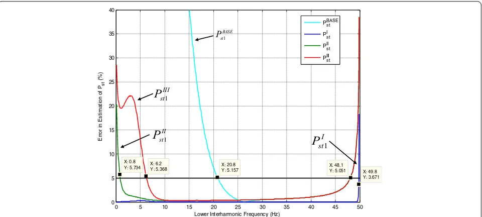
In Figure 5, the percentage errors (-PBASEst1 cyan curve,

-PUI

1 - blue curve, - PUII1 - green curve, - PUIII1 - red curve) versus the lower interharmonic frequency of the symmetric interharmonic pair are shown.

From Figure 5, it is possible to observe the following:

The blue curvePI_st1, in all the frequency range

analysed, gives the best results and only for the pair with the frequency of 49.9 Hz shows an error greater than 5% (black line). For this frequency, the error is caused mainly by the transient behaviour of the filters contained in the IEC flickermeter, which becomes non-negligible for interharmonic frequencies very close to the fundamental. This transient behaviour is not taken into account by pure frequency domain

methods differently from hybrid methods [12].

The green curvePII_st1and the red curvePIII_st1are

virtually indistinguishable for frequencies greater than 15 Hz. Below this frequency (as mentioned in

Section2), the impact of PU1_DC2on the total value

of PU1is non-negligible, and for this reason, in this

frequency range, the error committed by the analytical

estimationPII_st1is less than that produced byPIII_st1.

ThePII_st1estimation makes an error greater than 5%

(black line) for the pairs with frequencies higher than 48 Hz and lower than 0.8 Hz. The reason of these errors (in addition to the previously mentioned transient behaviour of the IEC flickermeter for interharmonic frequencies very close to the fundamental) is due to the AC

component of PU1, which is more consistent for

interharmonic tones withΔω1both close to the

fundamental frequency or close to zero.

ThePIII_st1estimation makes an error greater than 5%

(black line) for frequencies lower than 6.2 Hz and higher than 48 Hz. The reasons of the different trend of the red curve with respect to the other two

curves are the same as the ones mentioned in the previous point.

ThePBASE_st1 (cyan curve) makes an error almost equal

to thePII_st1and thePIII_st1for frequencies higher than

25 Hz, but for lower frequencies, as a result of the simplifying assumptions, the error diverges, rapidly reaching the 40% already for a frequency of 15 Hz.

3.2 Two pairs producing AM

The amplitude of the single pair of interharmonic tones has been chosen to produce singly a Pstequal to 1 (Figure 4). The frequency modulation of the two pairs, which are definedΔω1andΔω2in (14), has been chosen to vary be-tween 1 and 49 Hz, with steps of 1 Hz, and all their possible combinations have been evaluated. Since the Fourier period of the input signal is equal to 1 s, a DFT with a spectral resolution of 1 Hz is used.

Three different analytical estimations of the cumula-tivePst(Pst1+2) have been considered, all based on (15):

I)PUI1þ2¼PU1þ2¼PU1þ2 DCþPU1þ2 AC: ð20Þ

II) PUII1þ2¼PU1þ2 DC: ð21Þ

III) PUIII

1þ2¼PU1þPU2: ð22Þ

Obviously, the corresponding values of PI

st1þ2;PIIst1þ2 and PIIIst1þ2 have been calculated. Moreover, the results obtained implementing the analytical assessment pro-posed in [7] are reported and referred to asPBASEst1þ2.

In Figures 6, 7, 8 and 9, the percentage errors for the analytical estimation, PUI

1þ2;PUII1þ2;PUIII1þ2 andPBASEst1þ2are shown.

From these figures, it should be noted that

Thex-axis and they-axis represent the frequency of

lower interharmonic tone of the first and of the second interharmonic pair, respectively.

The most complete analytical estimationPI

st1þ2

(Figure6), for the most part of the cases analysed,

makes a mistake lower than 5% (light green squares). The cases with an error greater than the 5% occur essentially when the interaction between the two interharmonic pairs produces one or more

oscillating component of the PU1+2with an angular

frequency that the filterY(s) (6) is not able to

eliminate, which is not evaluated analytically.

These events occur when

i) Δω1≈Δω2(main diagonal);

Lower Interharmonic Frequency IH1 (Hz)

Figure 6Percentage errors in the evaluation ofPstof two pairs of interharmonic tones producing AM for PIst1þ2(20).

Lower Interharmonic Frequency IH1 (Hz)

)

Lower Interharmonic Frequency IH1 (Hz)

Figure 8Percentage errors in the evaluation ofPstof two pairs of interharmonic tones producing AM for PUIII1þ2(22).

Lower Interharmonic Frequency IH1 (Hz)

)

iii)Δω1≈2(ω1−Δω2) (in the top right corner);

iv)Δω2≈2(ω1−Δω1) (in the bottom left corner).

Comparing the results obtained forPI_st1þ2

(Figure6) and forPII_st1þ2(Figure7), it should be

noted that neglecting the effects of the AC components produced by the single

interharmonic pair increases the number of non-light green squares when

i) Δω1≈Δω2(main diagonal);

ii)Δω1≈2(ω1−Δω2) (in the top right corner) and

whenΔω2≈2(ω1−Δω1) (in the bottom left corner);

iii)Δω1= 1 (last column to the right) and whenΔω2= 1

(last column to the bottom).

Comparing the results obtained forPI_st1þ2

(Figure6) and forPIII_st1þ2(Figure8), it should be

noted that neglecting the effects of the

interactions between the two interharmonic pairs

on the DC component of the PU1+2are present

with a non-negligible entity when

i) Both the pairs have the lower interharmonic tone frequency lower than 15 Hz (in the top left corner);

ii)Δω1= 2(ω1−Δω2) (in the top right corner) or when

Δω2≈2(ω1−Δω1) (in the bottom left corner).

In similar mode to the case of an interharmonic

pair shown in Figure5, the analytical assessment

PBASEst1þ2(Figure9) makes errors very high

(sometimes even more than 100%) when one or both the pairs have the lower interharmonic tone with frequencies lower than 20 Hz.

Finally, it is worthwhile to note that from the

implementation point of view on a general PQ instrument, the proposed analytical approach requires only some manipulations, of different complexities depending on the level of

approximation desired (see (20), (21) and (22)),

of the spectra which are already evaluated by the PQ instrument for the harmonic and interharmonic analysis. On the other hand, the digital signal processing of the conventional IEC flickermeter requires the implementation of blocks 1 to 4 independently from the spectral analysis.

4 Conclusions

In this paper, a new analytical estimator for LF in the fre-quency domain, which is able to take into account also the frequency components neglected by the classical methods proposed in literature, has been proposed. The analytical solutions proposed apply for any generic sta-tionary signal affected by interharmonic distortion. The LF analytical estimator proposed has been applied to numerous numerical case studies with the goal of showing i) the correctness and the improvements of the analytical

approach proposed in respect with the other method pro-posed in literature and ii) the accuracy of the results com-pared to those obtained by means of the classical IEC flickermeter. The usefulness of the proposed analytical ap-proach is that it can be included in signal processing tools for interharmonic penetration studies for the integration of renewable energy sources in future smart grids.

The main outcomes of the paper are as follows:

In the presence of interharmonic tones in the

frequency range from DC to 15 Hz and from 85 to 100 Hz, the simplified assumptions made by classical methods proposed in literature can lead to very inaccurate results.

The analytical formulas can be used to perform

interharmonic penetration studies in transmission and distribution networks.

Future development of the research will be aimed to generalize the methodology adapted to interharmonic components at frequencies higher than 100 Hz which is proven to affect modern lighting systems different from incandescent bulbs.

5 Appendix A Analytical assessment of PU1_AC(t) With reference to (11), it is possible to demonstrate that the summands of (12) are equal to the following:

PU1 AC1 4Δω1ð Þt ≅

and that the summands of (13) are equal to the following:

PU1 AC2 2ω1−2Δω1ð Þt≅H

6 Appendix B Analytical Assessment of PU12_DC With reference to (15), PU12_DCcan be expressed as:

PU12 DC¼PU12 DC1þPU12 DC2: ð29Þ

It is possible to demonstrate that PU12_DC1is equal to:

PU12 DC1¼

ferent values according to the relationship between Δω1

andΔω2:

The authors declare that they have no competing interests.

Acknowledgements

The research activity discussed in this paper has been partially supported by the Project PON01_02582“Command, control, protection and supervision integrated system for production, transmission and distribution (ColAdMin integrated SCADA) of renewable and non renewable electrical energy, with field-device-interface, for rational use of electrical power”funded by the Italian Ministry for the Instruction, University and Research.

Received: 15 December 2014 Accepted: 16 February 2015

References

1. IEEE Task, Force on harmonics modeling and simulation, interharmonics: theory and modeling. IEEE Trans. Power Deliv.22(4), 2335–2348 (2007). doi:10.1109/TPWRD.2007.905505

2. IEC Standard 61000-4-15. Flickermeter—functional and design specifications (IEC, Geneva, Switzerland, Edition 2.0, 2010-07)

3. R Langella, A Testa, Amplitude and phase modulation effects of waveform distortion in power systems. J. Electrical Power Qual. Util.XIII(1), 25–32 (2007) 4. D Gallo, R Langella, A Testa,Light Flicker Prediction Based on Voltage Spectral

Analysis(Paper presented at the IEEE Porto Power Tech Conference, Porto, Portogallo, 2001), pp. 10–13

5. R Langella, A Testa, Power System Subharmonics, ed. by IEEE (Paper invited at the IEEE Power Engineering Society General Meeting 2005, S. Francisco, USAm, 2005)

7. A Hernandez, JG Mayordomo, R Asensi, LF Beites, A new frequency domain approach for flicker evaluation of arc furnaces. IEEE Trans. Power Deliv.

18(2), 631–638 (2003). doi:10.1109/TPWRD.2003.809733

8. CJ Wu, TH Fu, Effective voltage flicker calculation algorithm using indirect demodulation method. IEE P-Gener. Transm. D.150(4), 493–500 (2003). doi:10.1049/ip-gtd:20030302

9. T Keppler, NR Watson, J Arrilaga, S Chen, Theoretical assessment of light flicker caused by sub- and interharmonic frequencies. IEEE Trans. Power Deliv.18(1), 329–333 (2003). doi:10.1109/TPWRD.2002.806690 10. D Gallo, R Langella, C Landi, A Testa, On the use of the flickermeter

to limit low-frequency interharmonic voltages. IEEE Trans. Power Deliv.

23(4), 1720–1727 (2008). doi:10.1109/TPWRD.2008.2002842

11. N Kose, O Salor, New spectral decomposition based approach for flicker evaluation of electric arc furnaces. IET Gener. Transm. Dis.3(4), 393–411 (2009). doi:10.1049/iet-gtd.2008.0479

12. GW Chang, C Cheng-I, H Ya-Lun, A digital implementation of flickermeter in the hybrid time and frequency domains. IEEE Trans. Power Deliv.

24(3), 1475–1482 (2009). doi:10.1109/TPWRD.2009.2022673

13. A Hernández, JG Mayordomo, R Asensi, LF Beites, A method based on interharmonics for flicker propagation applied to arc furnaces. IEEE Trans. Power Deliv.20(3), 2334–2342 (2005). doi:10.1109/TPWRD.2005.848677 14. IEC standard 61000-4-7: General guide on harmonics and interharmonics

measurements, for power supply systems and equipment connected thereto (IEC, Geneva, Switzerland, Edition 2.0, 2002-08)

15. K Yang, MHJ Bollen, EO Anders Larsson, M Wahlberg, Measurements of harmonic emission versus active power from wind turbines. Electr. Pow. Syst. Res.108, 304–314 (2014). doi:10.1016/j.epsr.2013.11.025

16. F De Rosa, R Langella, A Sollazzo, A Testa, On the interharmonic components generated by adjustable speed drives. IEEE Trans. Power Deliv.

20(4), 2535–2543 (2005). doi:10.1109/TPWRD.2005.852313

17. R Carbone, F De Rosa, R Langella, A Testa, A new approach for the computation of harmonics and interharmonics produced by line-commutated AC/DC/AC converters. IEEE Trans. Power Deliv.

20(3), 2227–2234 (2005). doi:10.1109/TPWRD.2005.848448 18. R Langella, A Sollazzo, A Testa, A new approach for the computation of

harmonics and interharmonics produced by AC/DC/AC conversion systems with PWM inverters. Eur. T. Electr. Power20(1), 68–82 (2010). doi:10.1002/ etep.400

Submit your manuscript to a

journal and benefi t from:

7Convenient online submission 7Rigorous peer review

7Immediate publication on acceptance 7Open access: articles freely available online 7High visibility within the fi eld

7Retaining the copyright to your article